


Abstract
We present 294 pulsars found in GeV data from the Large Area Telescope (LAT) on the Fermi Gamma-ray Space Telescope. Another 33 millisecond pulsars (MSPs) discovered in deep radio searches of LAT sources will likely reveal pulsations once phase-connected rotation ephemerides are achieved. A further dozen optical and/or X-ray binary systems colocated with LAT sources also likely harbor gamma-ray MSPs. This catalog thus reports roughly 340 gamma-ray pulsars and candidates, 10% of all known pulsars, compared to ≤11 known before Fermi. Half of the gamma-ray pulsars are young. Of these, the half that are undetected in radio have a broader Galactic latitude distribution than the young radio-loud pulsars. The others are MSPs, with six undetected in radio. Overall, ≥236 are bright enough above 50 MeV to fit the pulse profile, the energy spectrum, or both. For the common two-peaked profiles, the gamma-ray peak closest to the magnetic pole crossing generally has a softer spectrum. The spectral energy distributions tend to narrow as the spindown power decreases to its observed minimum near 1033 erg s−1, approaching the shape for synchrotron radiation from monoenergetic electrons. We calculate gamma-ray luminosities when distances are available. Our all-sky gamma-ray sensitivity map is useful for population syntheses. The electronic catalog version provides gamma-ray pulsar ephemerides, properties, and fit results to guide and be compared with modeling results.

1. Introduction
Fewer than a dozen gamma-ray pulsars were known when the Fermi Gamma-ray Space Telescope was launched on 2008 June 11, and the extent and diversity of the population and its role in Galactic dynamics were subject to debate (Thompson 2008). Fermi's primary instrument, the Large Area Telescope (LAT; Atwood et al. 2009), quickly established that the gamma-ray population is large and varied and is the dominant GeV gamma-ray source class in the Milky Way (Abdo et al. 2010a; The First Fermi LAT Catalog of Gamma-ray Pulsars, hereafter 1PC). The 46 pulsars in 1PC (6 months of data) grew to 132 in 2PC (3 yr of data), the Second Fermi-LAT gamma-ray pulsar catalog (Abdo et al. 2013). This third gamma-ray pulsar catalog (based on 12 yr of data) characterizes 294 confirmed gamma-ray pulsars, and tabulates 33 millisecond pulsars (MSPs) for which gamma-ray pulsations have not yet been seen but likely will be once accurate rotation ephemerides are established. We further tabulate LAT sources likely to reveal new "spider" MSPs, and LAT sources colocated with known pulsars, some of which may ultimately reveal gamma-ray pulsations. Roughly 340 gamma-ray pulsars and candidates are thus now known, or about 10% of the >3400 currently known pulsars (see Table 1).
Table 1. Pulsar Varieties
| Category | Count | Subcount |
|---|---|---|
| Known rotation-powered pulsars (RPPs) a | 3436 | |
| with measured erg s−1 | 762 | |
| MSPs (P < 30 ms) | 681 | |
| with measured erg s−1 | 250 | |
| Field MSPs b | 427 | |
| MSPs in globular clusters c | 254 | |
| Gamma-ray pulsars in this catalog d | 294 | |
| Spectral fits (with free b parameter) f | 255 (116) | |
| Profile fits in ≥1, 2, 6 energy bands | 236, 167, 28 | |
| Young gamma-ray pulsars | 150 | |
| Radio-quiet e | 70 | |
| Gamma-ray MSPs | 144 | |
| Isolated, Binary | 32, 112 | |
| Discovered in LAT blind searches | 10 | |
| Radio-quiet | 6 | |
| Black Widows, Redbacks: | 32, 13 | |
| Radio MSPs discovered in LAT sources | 119 | |
| with gamma-ray pulsations | 78 | |
| waiting for ephemeris phase-connection d | 33 |


Notes.
a Includes the 3359 pulsars, which are all RPPs, in psrcat, the ATNF Pulsar Catalog (v1.69, Manchester et al. 2005), and as-yet unpublished discoveries. b http://astro.phys.wvu.edu/GalacticMSPs. c http://www.naic.edu/~pfreire/GCpsr. d Table 6 lists 39 MSPs discovered in radio searches of bright 4FGL sources with pulsar-like spectra. At least six were serendipitous. The rest will likely show pulsations once radio timing allows gamma-ray phase-folding. Table 5 lists additional pulsars colocated with 4FGL sources, some of which may reveal pulsations in the future. Table 15 lists 13 "spider" MSP candidates colocated with LAT sources. The number of detected gamma-ray pulsars thus likely exceeds 340, including unpulsed detections. e S1400 < 30 μJy, where S1400 is the radio flux density at 1400 MHz. f Sections 5 and 6 describe the pulse profile fits and energy spectral fits, respectively.Download table as: ASCIITypeset image
These results build on much previous work. GeV pulsations from the Crab were glimpsed using a balloon-borne instrument at the start of the 1970s (McBreen et al. 1973), followed by the pulsed detection of Vela by the SAS-2 satellite (Thompson et al. 1975). The COS-B satellite improved the measurements (Swanenburg et al. 1981). In the 1990s, EGRET on the Compton Gamma-Ray Observatory (CGRO) saw six GeV pulsars (Thompson et al. 1999), while a rare pulsar that is brighter below 100 MeV than above, PSR B1509−58 was detected with COMPTEL on CGRO (Kuiper et al. 1999; Abdo et al. 2010b). EGRET data revealed three other strong candidates: PSRs J0659+1414 (Ramanamurthy et al. 1996) and J1048−5832 (Kaspi et al. 2000), and the MSP PSR J0218+4232 (Kuiper et al. 2000). AGILE discovered gamma-ray pulsations from PSR J2021+3651 before Fermi's launch (Halpern et al. 2008). All 11 of these pulsars were quickly confirmed using LAT data, and are noted in Figure 1. Geminga, seen with EGRET, was undetected at radio wavelengths (Bignami & Caraveo 1996; Abdo et al. 2010c) and has turned out to be the prototype of about half of the young gamma-ray pulsars. The 294 pulsars reported here are more numerous than the 271 sources, all object classes combined, in the third EGRET source catalog (Hartman et al. 1999).

Figure 1. Cumulative number of known gamma-ray pulsars, beginning with the launch of Fermi. The crosses show the numbers included in the first (1PC) and second (2PC) catalogs of LAT pulsars and their publication dates. Some key discoveries are highlighted. See also Table 1.
Download figure:
Standard image High-resolution imageFigure 1 shows that the discovery rate since launch is steady. Table 1 breaks the numbers down by category. Long-term radio observations by the "Pulsar Timing Consortium" (Smith et al. 2008) enabled about half the discoveries and, importantly, also allowed for an unbiased sample of pulsars not seen in gamma-rays (Smith et al. 2019). The "Pulsar Search Consortium" (Ray et al. 2012), later joined by FAST (Li et al. 2018a; Wang et al. 2021) and the TRAPUM 107 project on MeerKAT (Clark et al. 2023a), discovered large numbers of radio MSPs at the positions of unidentified gamma-ray sources, leading to the subsequent detection of gamma-ray pulsations. Gamma-ray blind searches of unidentified sources revealed radio-quiet pulsars that make up a quarter of the current sample (see, e.g., Clark et al. 2017; Wu et al. 2018).
The discovery rate is sustained by innovations in how we detect pulsations. Ever-improving blind search algorithms (Pletsch & Clark 2014; Nieder et al. 2020a) allowed for the first discovery of a radio-quiet MSP (Clark et al. 2018). The increasingly sophisticated use of an optical companion's orbit reduces the parameter space searched using Einstein@Home 108 to discover gamma-ray MSPs in binary systems with perturbed orbits (Nieder et al. 2022). Another example is a method that allows photon weighting (see Section 2) even if the unpulsed gamma-ray source is undetected (Bruel 2019; Smith et al. 2019). Underlying all analysis efforts are the improved sensitivity and low-energy reach afforded by the Pass8 reconstruction method (Atwood et al. 2013; Bruel et al. 2018).
As a result, not just the numbers but the variety of gamma-ray pulsars continues to grow. The minimum spindown power is now 20× lower than the pre-launch expectation of 1034 erg s−1 (Smith et al. 2008). 109 The fastest known field MSP, PSR J0952−0607, was found at the location of a gamma-ray source and subsequently timed with LAT data (Bassa et al. 2017b; Nieder et al. 2019). A third globular cluster, NGC 6652, was found to have gamma-ray emission dominated by a single MSP, PSR J1835−3259B (Gautam et al. 2022b; Zhang et al. 2022), with a fourth recently reported, PSR J1717+4308A in M92 (Zhang et al. 2023). The gamma-ray flux and pulse profile of PSR J2021+4026 in the γ Cygni supernova remnant (SNR) changed during mode transitions in 2011 and 2018 (Allafort et al. 2013; Razzano et al. 2023). The LAT sees more than 40 "spider" MSPs and a dozen candidates (see Section 7), compact binary systems where the pulsar wind ablates its companion. Spiders fall into two categories: "black widows" have companion masses 0.01M⊙ < Mc < 0.05 M⊙ and orbital periods PB < 10 hr whereas "redbacks" have Mc > 0.2 M⊙ and PB < 1 day. Gamma-ray timing of 35 stable MSPs for over 12 yr usefully constrains the intensity of gravitational waves from supermassive black hole binaries in the hearts of distant galaxies. The upper limit should become a measurement in the coming years (Ajello et al. 2022). Following the methods initially applied to PSR J1555−2908 (Nieder et al. 2022), we may be poised to detect planets in multiyear orbits in several compact binary MSP systems.

This heterogeneous population can be classified by comparing the spin period (P) and the period derivative (), shown in Figure 2. Throughout this paper, we call pulsars in the main population "young" to distinguish them from the much older MSPs, thought to be spun up to rapid periods via accretion from a companion (Alpar et al. 1982), although, e.g., the accretion-induced collapse of white dwarfs might also create MSPs (Gautam et al. 2022a).


Figure 2. Pulsar spindown rate, , vs. the rotation period P. Green dots indicate young, radio-loud (RL) gamma-ray pulsars and blue squares show "radio-quiet" (RQ) pulsars, defined as S1400 < 30 μJy, where S1400 is the radio flux density at 1400 MHz. Red triangles are millisecond gamma-ray pulsars. Black dots indicate pulsars phase-folded in gamma-rays without significant pulsations. Phase-folding was not done for pulsars shown by gray dots. Orange triangles are radio MSPs discovered at the positions of previously unassociated LAT sources, hidden by red triangles when gamma pulsations were subsequently found. The rest are listed in Table 6, and plotted with when is unavailable. The solid black diagonal is the radio deathline of Equation (4) of Zhang et al. (2000). Shklovskii corrections to have been applied only to gamma-ray MSPs with measured proper motion (see Section 4.3).


Download figure:
Standard image High-resolution imageAll known gamma-ray pulsars are rotation-powered pulsars (RPPs): LAT has not yet detected accretion-powered pulsars nor the magnetars that populate the upper-right portion of the plane, for which the dominant energy source is magnetic field decay (Parent et al. 2011). An interesting exception is an LAT detection of a few photons for a few minutes from an extragalactic magnetar giant flare (Ajello et al. 2021a). The locations of all 294 gamma-ray pulsars on the sky are shown in Figure 3. The diagram shows diagonal lines of constant , τc , and BS derived from the timing information as follows. For an orthogonal rotator, the magnetic field on the neutron star surface at the magnetic equator (the rotation pole) is . The "characteristic age" assumes that magnetic dipole braking is the only energy-loss mechanism, that the magnetic moment and inclination do not change, and that the initial spin period was much less than the current period. τc thus approximates true age well for some young pulsars, and poorly for MSPs. We set the neutron star radius to RNS = 10 km, and c is the speed of light in a vacuum.


Figure 3. Pulsar sky map in Galactic coordinates (Hammer projection). Symbols are the same as in Figure 2.
Download figure:
Standard image High-resolution imageThe fourth Fermi-LAT source catalog (Abdollahi et al. 2020), and specifically Data Release 3 (DR3; Abdollahi et al. 2022, hereafter 4FGL) 110 characterizes 6658 point and extended sources using 12 yr of LAT data. Half of the sources are various blazar classes of active galactic nuclei, but a third remain unassociated with objects known at other wavelengths. Radio and gamma-ray pulsation searches at the positions of unidentified sources have yielded fully half of the gamma-ray pulsars. The discoveries continue, as detailed in Sections 3 and 7. The 4FGL spectral, flux, and variability measurements are used throughout this work for the pulsar searches and characterization.
We provide the pulsar catalog in FITS 111 and spreadsheet file formats, along with other information here as well as on the Fermi Science Support Center (FSSC) servers. 112 Appendix D provides a description of this material.
2. Observations
Atwood et al. (2009) described the Fermi LAT, and Abdo et al. (2009a), Ackermann et al. (2012a), and Ajello et al. (2021b) reported on-orbit performance. Fermi carries another instrument, the Gamma-ray Burst Monitor (Meegan et al. 2009), which was not used to prepare this catalog.
The LAT is a pair-production telescope composed of a 4 × 4 grid of towers. Each tower consists of a stack of tungsten foil converters interleaved with silicon-strip particle tracking detectors, mated with a hodoscopic cesium-iodide calorimeter. A segmented plastic scintillator anticoincidence detector covers the grid to help discriminate charged particle backgrounds from gamma-ray photons. The LAT field of view is ∼2.4 sr. For most of the Fermi mission, the primary operational mode has been a sky survey where the satellite rocks between a pointing above the orbital plane and one below the plane after each orbit. In this mode, the entire sky is imaged every two orbits (∼3 hr) and any given point on the sky is observed ∼1/6th of the time. For 1 yr, beginning 2013 December, the normal survey mode was changed to favor exposure to the Galactic center region. 113 Survey mode was again modified after a solar panel rotation drive stopped moving on 2018 March 16, detailed in Ajello et al. (2021b).
The LAT is sensitive to gamma-rays with energies E from 20 MeV to over 300 GeV, with an on-axis effective area of ∼8000 cm2 above 1 GeV. Multiple Coulomb scattering of the electron–positron pairs created by converted gamma-rays degrades the per-photon angular resolution, with the average 68% containment radius varying as E−0.8 from 5° at 100 MeV to 0 1 at 10 GeV.
114
1 at 10 GeV.
114
This energy-dependent point-spread function, the backgrounds from the complex diffuse emission and nearby sources, and the source spectrum are encapsulated in the photon weights (wi , Kerr 2011), which give the probability that a photon originates from a particular source. Weights are used to optimize pulsed signal significance while minimizing event selection trials penalties. This powerful tool has been extended ("simple weights" and "model weights") to sky locations with no point source (Bruel 2019). Weighting is used for all of the discovery techniques (Section 3), and to characterize the pulse profiles (Section 5).
Events recorded by the LAT have time stamps derived from GPS clocks integrated into the satellite's Guidance, Navigation, and Control (GNC) subsystem, accurate to ≈ 300 ns relative to UTC (Abdo et al. 2009a; Ajello et al. 2021b). GNC provides the instantaneous spacecraft position with ≈60 m accuracy. Generally, we compute pulsar rotational phases ϕi using Tempo2 (Hobbs et al. 2006) with the fermi plug-in (Ray et al. 2011), or with PINT (Luo et al. 2021). These use the recorded times and spacecraft positions combined with a pulsar rotational ephemeris (specified in a Tempo2 parameter, or "par," file). The timing chain from the instrument clocks through the barycentering, and epoch folding software is accurate to better than a microsecond (Smith et al. 2008).
We use different data selections and processing for the various analyses presented here, though all cases make use of "Source" class events reconstructed using Pass8 revision 3 (Atwood et al. 2013; Bruel et al. 2018). The pulsation searches and pulsar timing described in Section 3 generally make use of all available data at the time of analysis and employ a variety of data processing methods. The effects of this heterogeneity on, e.g., pulsar discovery efficiency or pulse profile inference are minor, and we do not attempt to provide further details.
For the pulse profiles (see Section 5), the data span 11.8 yr, from MJD 54682 (2008 August 4, when LAT data taking began) to MJD 59000 (2020 May 31). We exclude gamma-rays collected when the LAT was not in nominal science operations mode or when the spacecraft rocking angle exceeded 52°, and we accept photons with reconstructed energies from 0.05 to 100 GeV, within 15° of the pulsar positions. We used Model Weights, requiring weights wi > 0.001.
The spectral measurements (see Section 6) use the same data set as 4FGL-DR3. In brief, the data span 12 yr, to MJD 59063 (2020 August 2) and are selected with energies 50 MeV to 1 TeV. The catalog analysis further uses a heterogeneous zenith angle cut ranging from 80° for energies below 100 MeV to 105° above 1 GeV.
3. Discovery and Timing
Inclusion in the main catalog requires a statistically significant pulsation detection in the Fermi LAT gamma-ray data. The following subsections describe the paths to detection, as well as a brief description of gamma-ray timing that often strengthens the initial signal.
In all cases, detecting and characterizing pulsations requires a rotation ephemeris (or a "timing model") to convert photon arrival times ti to neutron star rotational phases ϕi . This "folding," which "stacks" photons at the same rotational phase, allows a pulse to rise above the background since ≪1 photons are collected per pulse even from the brightest pulsars (Kerr 2022). We detect pulsations with the H-test (de Jager et al. 1989; de Jager & Büsching 2010), a statistical test for discarding the null hypothesis that a set of photon phases is uniformly distributed. For Nγ gamma-rays, the m = 20 harmonic weighted version of the H-test statistic (Kerr 2011) is

with

and αkw and βkw are the empirical trigonometric coefficients and . The w subscripts indicate that this is a photon-weighted version of the test, and the wi are the photon weights, evaluated via spectral analysis (see also 2PC, Abdo et al. 2013). For m = 20, which we adopt universally, the cumulative distribution function for H in the asymptotic limit is (Kerr 2011), and 3σ, 4σ, and 5σ thresholds correspond to H = 14, H = 24, and H = 36. The H-test is unbinned, well suited to the extremely sparse gamma-ray pulsar data: the LAT often detects only one photon in tens of thousands (millions, for MSPs) of pulsar rotations. Bruel (2019) gave corrections for small photon counts. Pulsars with narrow, sharp peaks are easier to detect than pulsars with broad peaks (see Figure 5 of Hou et al. 2014). All pulsars in our sample are detected with m = 8. Using m = 20 incurs little computational cost and insures sensitivity to putative exotic profile shapes. Kerr (2011) also showed that large m does not cause false-positive detections.


Figure 4 highlights some aspects of gamma-ray phase folding. Figure 9 and Appendix B show other example profiles. The top-most frame shows a weighted phase histogram, duplicated over a second rotation. Section 5 describes the profile fit overlaid in blue. The phase-aligned 1.4 GHz radio pulse overlaid in red comes from the radio timing observations used to create the rotation ephemeris, in this specific case by Parthasarathy et al. (2019). The horizontal dashed line shows the gamma-ray background level, estimated from the photon weights as , the sum of the expected contribution to the weights of background photons not associated with the pulsar. A phase histogram baseline exceeding the background level may indicate the presence of unpulsed magnetospheric emission. Section 5.1 gives details.

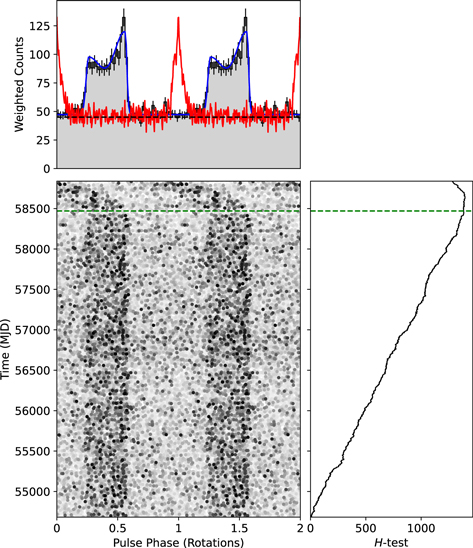
Figure 4. Top: gamma-ray phase histogram for PSR J1648-4611 discovered by Kramer et al. (2003), overlaid with the 1.4 GHz profile (red) obtained during Parkes radio telescope timing (Parthasarathy et al. 2019). The blue curve shows a fit to the histogram, and the horizontal dashed line is an estimate of the background level (see Section 5.1). Bottom-left: phaseogram over the course of the mission. Dots indicate photons, with the grayscale set according to the photon weight. Right: H-test significance accumulated over the course of the mission. The green horizontal dashed line shows when the ephemeris validity finishes (see Section 3.1).
Download figure:
Standard image High-resolution imageThe next frame below it shows the phase drifting after the last radio time of arrival (ToA) used to model the neutron star rotation, indicated by the green horizontal dashed line. The start of this timing model's "validity" range, before Fermi's launch, is not shown. Pulsars with irregular spindown, as for this young high- pulsar, require extra parameters to model the rotation, and accuracy of the extrapolation past the validity range rapidly degrades. Stable pulsars can be modeled with few parameters, often accurately predicting the neutron star rotation for years before and/or after validity. The right-hand frame shows the weighted H-test increasing as data accumulated over the years, a nearly straight line for most pulsars. Changes in slope can result from phase drifts, as in this case, or from increased background due to, e.g., a nearby flaring blazar (see Section 6.6), or from changes in the LAT's exposure to the pulsar's sky position. Exposure per unit time increased for this pulsar during 2014 (mid-year was MJD 56810) when LAT pointed more frequently toward the Galactic center, visible in the time versus phase plot, without however affecting the H-test growth. Smith et al. (2019) showed simulations for which Poisson fluctuations in the very low rate of photon arrivals for pulsars near detection threshold significantly perturb the H-test time evolution. Slope variations due to pulsar flux changes nearly never happen: rare exceptions are the young pulsar PSR J2021+4026 (Allafort et al. 2013; Razzano et al. 2023) and transitional MSPs like PSR J1023+0038 (see Stappers et al. 2014, and Appendix A) and J1227−4853 (Johnson et al. 2015; Roy et al. 2015), which lack detectable gamma-ray pulsations during their accretion states.

If different analyses were tried, the number of trials must be accounted for in the pulsation significance calculation, requiring a higher H-test value to claim a detection. Before the advent of photon weighting, we sometimes varied the minimum energy and/or the angular extent of our data set, to explore the pulsar's spectral hardness and local background level. Using a LAT source's measured spectrum to calculate weights allows one single trial for this parameter space.
When the source spectrum is too faint to measure, we use "simple weights" with a parameter μw of unknown optimal value, and thus, possible additional trials. The μw parameter is the logarithm of the energy at which the log-Gaussian weighting function peaks. Since Smith et al. (2019), we have been using six trials for simple weight gamma-ray pulsation searches using radio or X-ray ephemerides, and an H-test > 25 (p = 4.7 × 10⁻⁵, or > 4.1σ) detection threshold. We fold the entire data set three times, using μw = (3.2, 3.6, 4.0), and three more times restricting the data to the ephemeris validity period. Although these six trials are not independent, a conservative estimate for the chance probability for a false-positive detection with an H-test > 25 threshold is 6 × 4.7 × 10−5, or 0.3 for a sample of 1000 pulsars. In 2PC we required an H-test > 36 (>5σ). Smith et al. (2019) discovered 16 new gamma-ray pulsars, in part because of this refined, relaxed threshold. Several more pulsars in this catalog were later found in the same way.
This prescription may miss some pulsars if the ephemeris extrapolates well enough that the accumulation of additional data beyond the validity range yields H > 25, but poorly enough that the full data yield H < 25. Such cases also arise from positive fluctuations, so we avoid further trials factors by limiting our search to the two combinations just described.
As further explained in Section 3.4, when the ephemeris is established independently of the LAT, using radio or X-ray observations (Section 3.1), the pulsar can be up to 20 times fainter in gamma-rays than if an unidentified LAT point source (Section 3.2) guides a "blind" gamma-ray search. Once pulsations are found during some epoch of LAT data, gamma-ray timing can extend and improve the ephemeris (Section 3.5).
Using the above detection criteria, we report 294 gamma-ray pulsars in the breakdown tabulated in Table 1 with their distribution on the sky shown in Figure 3. The 150 young pulsars are named in Table 2, and the 144 MSPs are in Table 3. The new pulsars in 3PC were mostly more "difficult" to discover than those reported in the earlier catalogs. For pulsars found with just a few foldings using a radio ephemeris, discussed in Section 3.1, difficulty stems from their extreme faintness (<1 photon per month): an analysis using many trials (for example, from exploring different data intervals) yields significance too low to distinguish from statistical fluctuations. Furthermore, we continue to discover radio MSPs at the positions of unidentified FGL sources, described in Section 3.3. These are difficult both in radio, because of eclipses, scintillation, and intrinsic faintness, and in gamma-rays if their signal-to-noise ratio (S/N) is low and the ephemeris validity is brief, that is, if the radio observations cover only a few years of the LAT mission. The blind searches, discussed in Section 3.4, are now finding MSPs, including those with short, varying orbital periods, feared as perhaps impossible before launch (Ransom 2007). These searches require many orders of magnitude more computing power than for young pulsars. The catalog includes 44 "spider" systems, and in Section 7.1 we tabulate several candidates colocated with gamma-ray sources, for which pulsations will likely be seen in the coming years. Timing models for "noisy" pulsars require many parameters, which presents difficulty in maintaining a coherent timing solution, e.g., with frequent radio monitoring. Our methodical pursuit of ever more difficult gamma-ray pulsars in the LAT's unbiased all-sky data set means that our notion of gamma-ray pulsars is greatly enriched compared to 1PC.
Table 2. Some Parameters of Young LAT-detected Pulsars
| PSR | Codes | l | b | P | S1400 | ||
|---|---|---|---|---|---|---|---|
| (°) | (°) | (ms) | (10−15) | (erg s−1) | (mJy) | ||
| J0002+6216 | GUr | 117.33 | −0.07 | 115.4 | 6.0 | 153.0 | 0.02 |
| J0007+7303 | Gq | 119.66 | 10.46 | 315.9 | 355.92 | 445.0 | <0.005 |
| J0106+4855 | GUr | 125.47 | −13.87 | 83.2 | 0.4 | 29.4 | 0.01 |
| J0117+5914 | Rr | 126.28 | −3.46 | 101.4 | 5.8 | 221.0 | 0.30 |
| J0139+5814 | Rr | 129.22 | −4.04 | 272.5 | 10.7 | 20.9 | 4.60 |
| J0205+6449 | Xrx | 130.72 | 3.08 | 65.7 | 192.1 | 26688.0 | 0.05 |
| J0248+6021 | Rr | 136.90 | 0.70 | 217.1 | 55.2 | 212.0 | 13.70 |
| J0357+3205 | GUq | 162.76 | −16.01 | 444.1 | 13.10 | 5.90 | <0.004 |
| J0359+5414 | GUq | 148.23 | 0.88 | 79.4 | 16.7 | 1317.0 | |
| J0514−4408 | Rr | 249.51 | −35.36 | 320.3 | 2.0 | 2.45 | 0.71 |
| J0534+2200 | RErx | 184.56 | −5.78 | 33.7 | 420.2 | 435319.0 | 14.00 |
| J0540−6919 | Xrx | 279.72 | −31.52 | 50.6 | 478.9 | 145529.0 | 0.10 |
| J0554+3107 | GUq | 179.06 | 2.70 | 465.0 | 142.60 | 56.0 | <0.066 |
| J0622+3749 | GUq | 175.88 | 10.96 | 333.2 | 25.42 | 27.1 | <0.012 |
| J0631+0646 | GUr | 204.68 | −1.24 | 111.0 | 3.6 | 104.0 | 0.025a |
| J0631+1036 | Rr | 201.22 | 0.45 | 287.8 | 102.7 | 170.0 | 1.11 |
| J0633+0632 | GUq | 205.09 | −0.93 | 297.4 | 79.57 | 119.0 | <0.003 |
| J0633+1746 | XExq | 195.13 | 4.27 | 237.1 | 10.97 | 32.5 | <0.507 |
| J0659+1414 | RErx | 201.11 | 8.26 | 384.9 | 55.0 | 38.0 | 2.70 |
| J0729−1448 | Rr | 230.39 | 1.42 | 251.7 | 113.4 | 280.0 | 0.83 |
| J0729−1836 | Rr | 233.76 | −0.34 | 510.2 | 18.9 | 5.63 | 1.90 |
| J0734−1559 | GUq | 232.06 | 2.02 | 155.1 | 12.51 | 132.0 | <0.005 |
| J0742−2822 | Rr | 243.77 | −2.44 | 166.8 | 16.7 | 141.0 | 26.00 |
| J0744−2525 | GUq | 241.35 | −0.73 | 92.0 | 1.0 | 48.3 | |
| J0802−5613 | GUq | 269.98 | −13.19 | 274.1 | 2.8 | 5.30 | |
| J0834−4159 | Rr | 260.89 | −1.04 | 121.1 | 4.3 | 95.1 | 0.28 |
| J0835−4510 | RErx | 263.55 | −2.79 | 89.4 | 122.3 | 6763.0 | 1050.00 |
| J0908−4913 | Rr | 270.27 | −1.02 | 106.8 | 15.1 | 490.0 | 20.00 |
| J0922+0638 | Rr | 225.42 | 36.39 | 430.6 | 13.7 | 6.77 | 10.00 |
| J0940−5428 | Rr | 277.51 | −1.29 | 87.6 | 32.8 | 1928.0 | 0.66 |
| J1016−5857 | Rr | 284.08 | −1.88 | 107.4 | 80.4 | 2563.0 | 0.90 |
| J1019−5749 | Rr | 283.84 | −0.68 | 162.5 | 20.1 | 184.0 | 3.80 |
| J1023−5746 | GUq | 284.17 | −0.41 | 111.5 | 379.89 | 10820.0 | <0.030 |
| J1028−5819 | Rr | 285.06 | −0.50 | 91.4 | 14.2 | 734.0 | 0.24 |
| J1044−5737 | GUq | 286.57 | 1.16 | 139.0 | 54.57 | 801.0 | <0.020 |
| J1048−5832 | REr | 287.43 | 0.58 | 123.7 | 95.5 | 1992.0 | 9.10 |
| J1055−6028 | Rr | 289.13 | −0.74 | 99.7 | 29.5 | 1176.0 | 0.95 |
| J1057−5226 | RErx | 285.98 | 6.65 | 197.1 | 5.8 | 30.1 | 4.40 |
| J1057−5851 | GUq | 288.61 | 0.80 | 620.4 | 100.6 | 16.6 | |
| J1105−6037 | GUq | 290.24 | −0.40 | 194.9 | 21.8 | 116.0 | |
| J1105−6107 | Rr | 290.49 | −0.85 | 63.2 | 15.8 | 2475.0 | 1.20 |
| J1111−6039 | GUq | 291.02 | −0.11 | 106.7 | 195.2 | 6346.0 | |
| J1112−6103 | Rr | 291.22 | −0.46 | 65.0 | 31.5 | 4537.0 | 2.30 |
| J1119−6127 | Rrx | 292.15 | −0.54 | 409.1 | 4042.4 | 2330.0 | 1.09 |
| J1124−5916 | Rrx | 292.04 | 1.75 | 135.5 | 751.5 | 11914.0 | 0.08 |
| J1135−6055 | GUq | 293.79 | 0.58 | 114.5 | 78.23 | 2057.0 | <0.030 |
| J1139−6247 | GUq | 294.79 | −1.06 | 120.4 | 4.1 | 91.6 | |
| J1151−6108 | Rr | 295.81 | 0.91 | 101.6 | 10.3 | 386.0 | 0.06 |
| J1203−6242 | GUq | 297.52 | −0.34 | 100.6 | 44.1 | 1709.0 | |
| J1208−6238 | GUq | 297.99 | −0.18 | 440.7 | 3309.57 | 1526.0 | <0.017 |
| J1224−6407 | Rr | 299.98 | −1.41 | 216.5 | 5.0 | 19.3 | 8.90 |
| J1231−5113 | GUq | 299.76 | 11.52 | 206.4 | 0.1 | 0.525 | |
| J1231−6511 | GUq | 300.87 | −2.40 | 247.4 | 28.4 | 74.0 | |
| J1253−5820 | Rr | 303.20 | 4.53 | 255.5 | 2.1 | 4.98 | 4.10 |
| J1341−6220 | Rr | 308.73 | −0.03 | 193.4 | 253.0 | 1379.0 | 2.70 |
| J1350−6225 | GUq | 309.73 | −0.34 | 138.2 | 8.9 | 132.0 | |
| J1357−6429 | Rrx | 309.92 | −2.51 | 166.2 | 354.4 | 3047.0 | 0.52 |
| J1358−6025 | GUq | 311.11 | 1.37 | 60.5 | 3.0 | 536.0 | |
| J1410−6132 | Rr | 312.19 | −0.09 | 50.1 | 31.8 | 10000.0 | 1.90 |
| J1413−6205 | GUq | 312.37 | −0.74 | 109.7 | 27.39 | 818.0 | <0.024 |
| J1418−6058 | GUq | 313.32 | 0.13 | 110.6 | 171.00 | 4992.0 | <0.029 |
| J1420−6048 | Rrx | 313.54 | 0.23 | 68.2 | 82.4 | 10250.0 | 1.19 |
| J1422−6138 | GUq | 313.52 | −0.66 | 341.0 | 96.79 | 96.4 | <0.060 |
| J1429−5911 | GUq | 315.26 | 1.30 | 115.8 | 23.88 | 606.0 | <0.021 |
| J1447−5757 | GUq | 317.85 | 1.51 | 158.7 | 11.7 | 115.0 | |
| J1459−6053 | GUqx | 317.89 | −1.79 | 103.2 | 25.26 | 908.0 | <0.037 |
| J1509−5850 | Rr | 319.97 | −0.62 | 88.9 | 9.2 | 516.0 | 0.21 |
| J1513−5908 | XErx | 320.32 | −1.16 | 151.6 | 1526.2 | 17290.0 | 1.43 |
| J1522−5735 | GUq | 322.05 | −0.41 | 204.3 | 62.46 | 289.0 | <0.034 |
| J1528−5838 | GUq | 322.17 | −1.75 | 355.7 | 24.8 | 21.7 | |
| J1531−5610 | Rr | 323.90 | 0.03 | 84.2 | 13.8 | 911.0 | 0.87 |
| J1614−5048 | Rr | 332.21 | 0.17 | 231.9 | 492.0 | 1557.0 | 4.10 |
| J1615−5137 | GUq | 331.76 | −0.54 | 179.3 | 10.6 | 72.8 | |
| J1620−4927 | GUq | 333.89 | 0.41 | 171.9 | 10.49 | 81.5 | <0.040 |
| J1623−5005 | GUq | 333.72 | −0.31 | 85.1 | 4.2 | 266.0 | |
| J1624−4041 | GUq | 340.56 | 6.15 | 167.9 | 4.7 | 39.4 | |
| J1641−5317 | GUq | 333.29 | −4.56 | 175.1 | 3.7 | 27.2 | |
| J1646−4346 | Rr | 341.11 | 0.98 | 231.7 | 111.8 | 355.0 | 1.25 |
| J1648−4611 | Rr | 339.44 | −0.79 | 165.0 | 23.7 | 208.0 | 0.61 |
| J1650−4601 | GUq | 339.78 | −0.95 | 127.1 | 15.1 | 291.0 | |
| J1702−4128 | Rr | 344.74 | 0.12 | 182.2 | 52.3 | 341.0 | 1.17 |
| J1705−1906 | Rr | 3.19 | 13.03 | 299.0 | 4.1 | 6.11 | 5.66 |
| J1709−4429 | RErx | 343.10 | −2.69 | 102.5 | 94.8 | 3475.0 | 12.10 |
| J1714−3830 | GUq | 348.44 | 0.14 | 84.1 | 70.3 | 4657.0 | |
| J1718−3825 | Rr | 348.95 | −0.43 | 74.7 | 13.2 | 1248.0 | 1.70 |
| J1730−3350 | Rr | 354.13 | 0.09 | 139.5 | 84.1 | 1222.0 | 4.30 |
| J1731−4744 | Rr | 342.56 | −7.67 | 829.9 | 163.5 | 11.3 | 27.00 |
| J1732−3131 | GUr | 356.31 | 1.01 | 196.5 | 28.0 | 145.0 | 0.05 |
| J1736−3422 | GUq | 354.33 | −1.18 | 346.9 | 65.5 | 62.0 | |
| J1739−3023 | Rr | 358.09 | 0.34 | 114.4 | 11.4 | 300.0 | 1.01 |
| J1740+1000 | Rr | 34.01 | 20.27 | 154.1 | 21.3 | 230.0 | 2.70 |
| J1741−2054 | GUrx | 6.42 | 4.91 | 413.7 | 17.0 | 9.48 | 0.16 |
| J1742−3321 | GUq | 355.85 | −1.69 | 143.3 | 1.3 | 17.0 | |
| J1746−3239 | GUq | 356.96 | −2.17 | 199.5 | 6.56 | 32.6 | <0.034 |
| J1747−2958 | Rrx | 359.31 | −0.84 | 98.8 | 61.3 | 2506.0 | 0.25 |
| J1748−2815 | GUq | 0.91 | −0.19 | 100.2 | 3.5 | 138.0 | |
| J1757−2421 | Rr | 5.28 | 0.06 | 234.1 | 12.7 | 39.2 | 7.20 |
| J1801−2451 | Rr | 5.27 | −0.87 | 125.0 | 89.5 | 1810.0 | 1.46 |
| J1803−2149 | GUq | 8.14 | 0.19 | 106.3 | 19.50 | 640.0 | <0.024 |
| J1809−2332 | Gq | 7.39 | −2.00 | 146.8 | 34.39 | 429.0 | <0.025 |
| J1813−1246 | GUq | 17.24 | 2.44 | 48.1 | 17.56 | 6238.0 | <0.017 |
| J1816−0755 | Rr | 21.87 | 4.09 | 217.6 | 6.5 | 24.8 | 0.17 |
| J1817−1742 | GUq | 13.34 | −0.70 | 149.7 | 20.6 | 241.0 | |
| J1826−1256 | Gxq | 18.56 | −0.38 | 110.2 | 120.95 | 3564.0 | <0.013 |
| J1827−1446 | GUq | 17.08 | −1.50 | 499.2 | 45.3 | 14.4 | |
| J1828−1101 | Rr | 20.49 | 0.04 | 72.1 | 14.8 | 1562.0 | 2.30 |
| J1831−0952 | Rr | 21.90 | −0.13 | 67.3 | 8.3 | 1078.0 | 0.35 |
| J1833−1034 | Rr | 21.50 | −0.89 | 61.9 | 202.0 | 33623.0 | 0.07 |
| J1835−1106 | Rr | 21.22 | −1.51 | 165.9 | 20.6 | 178.0 | 2.50 |
| J1836+5925 | Gq | 88.88 | 25.00 | 173.3 | 1.50 | 11.4 | <0.004 |
| J1837−0604 | Rr | 25.96 | 0.27 | 96.3 | 44.9 | 1982.0 | 0.75 |
| J1838−0537 | GUq | 26.51 | 0.21 | 145.8 | 450.71 | 5746.0 | <0.017 |
| J1841−0524 | Rr | 27.02 | −0.33 | 445.8 | 233.2 | 103.0 | 0.20 |
| J1844−0346 | GUq | 28.79 | −0.19 | 112.9 | 154.7 | 4249.0 | |
| J1846+0919 | GUq | 40.69 | 5.34 | 225.6 | 9.93 | 34.2 | <0.005 |
| (J1846−0258)b | Xxq | 29.71 | −0.24 | 326.6 | 7107.1 | 8055.0 | |
| J1853−0004 | Rr | 33.09 | −0.47 | 101.4 | 5.6 | 210.0 | 0.70 |
| J1856+0113 | Rr | 34.56 | −0.50 | 267.5 | 205.9 | 424.0 | 0.19 |
| J1857+0143 | Rr | 35.17 | −0.57 | 139.8 | 31.0 | 448.0 | 0.74 |
| J1906+0722 | GUq | 41.22 | 0.03 | 111.5 | 35.86 | 1020.0 | <0.021 |
| J1907+0602 | Gr | 40.18 | −0.89 | 106.6 | 86.5 | 2814.0 | 0.00 |
| J1913+0904 | Rr | 43.50 | −0.68 | 163.3 | 17.6 | 159.0 | 0.40 |
| J1913+1011 | Rr | 44.48 | −0.17 | 35.9 | 3.4 | 2882.0 | 0.90 |
| J1925+1720 | Rr | 52.18 | 0.59 | 75.7 | 10.5 | 954.0 | 0.07 |
| J1928+1746 | Rr | 52.93 | 0.11 | 68.7 | 13.2 | 1602.0 | 0.28 |
| J1932+1916 | GUq | 54.66 | 0.08 | 208.2 | 93.17 | 407.0 | <0.075 |
| J1932+2220 | Rr | 57.36 | 1.55 | 144.5 | 57.0 | 746.0 | 1.20 |
| J1935+2025 | Rr | 56.05 | −0.05 | 80.0 | 60.4 | 4638.0 | 0.50 |
| J1952+3252 | RErx | 68.77 | 2.82 | 39.5 | 5.8 | 3723.0 | 1.00 |
| J1954+2836 | GUq | 65.24 | 0.38 | 92.7 | 21.16 | 1048.0 | <0.005 |
| J1954+3852 | Rr | 74.04 | 5.70 | 352.9 | 6.6 | 5.93 | 1.07 |
| J1957+5033 | GUq | 84.58 | 11.01 | 374.8 | 7.08 | 5.31 | <0.010 |
| J1958+2846 | GUq | 65.88 | −0.35 | 290.4 | 211.89 | 341.0 | <0.006 |
| J2006+3102 | Rr | 68.67 | −0.53 | 163.7 | 24.9 | 223.0 | 0.27 |
| J2017+3625 | GUq | 74.51 | 0.39 | 166.7 | 1.4 | 11.6 | |
| J2021+3651 | Rr | 75.22 | 0.11 | 103.7 | 94.8 | 3351.0 | 0.10 |
| J2021+4026 | Gq | 78.23 | 2.09 | 265.3 | 55.60 | 117.0 | <0.020 |
| J2022+3842 | Xrx | 76.89 | 0.96 | 48.6 | 86.2 | 29707.0 | 0.11 |
| J2028+3332 | GUq | 73.36 | −3.01 | 176.7 | 4.86 | 34.8 | <0.005 |
| J2030+3641 | RUr | 76.12 | −1.44 | 200.1 | 6.5 | 32.0 | 0.15 |
| J2030+4415 | GUq | 82.34 | 2.89 | 227.1 | 5.05 | 17.0 | <0.008 |
| J2032+4127 | GUbr | 80.22 | 1.03 | 143.2 | 11.6 | 156.0 | 0.23 |
| J2043+2740 | Rr | 70.61 | −9.15 | 96.1 | 1.2 | 55.0 | 0.34 |
| J2055+2539 | GUq | 70.69 | −12.52 | 319.6 | 4.10 | 4.96 | <0.007 |
| J2111+4606 | GUq | 88.31 | −1.45 | 157.8 | 162.63 | 1632.0 | <0.013 |
| J2139+4716 | GUq | 92.63 | −4.02 | 282.8 | 1.78 | 3.11 | <0.014 |
| J2208+4056 | Rr | 92.57 | −12.11 | 637.0 | 5.3 | 0.807 | 0.04 |
| J2229+6114 | Rrx | 106.65 | 2.95 | 51.7 | 75.3 | 21557.0 | 0.25 |
| J2238+5903 | GUq | 106.56 | 0.48 | 162.7 | 96.85 | 887.0 | <0.011 |
| J2240+5832 | Rr | 106.57 | −0.11 | 139.9 | 15.3 | 219.0 | 2.70 |


Note. Column 2 gives the discovery and detection codes: G = discovered in Fermi-LAT gamma-ray data, R = discovered in the radio and/or gamma-ray pulsations detected using the radio ephemeris, X = discovered in the X-ray and/or gamma-ray pulsations detected using the X-ray ephemeris, E = pulsar was detected in gamma-rays by EGRET/COMPTEL, P = discovered by the Pulsar Search Consortium, U = discovered using a Fermi-LAT seed position, r = pulsations detected in the radio band, x = pulsations detected in the X-ray band, b = binary, and q = no radio detection. In Pletsch et al. (2013) and Kerr et al. (2015), PSR J1522−5735 erroneously has half the spin period shown here and 4× higher . Our larger gamma-ray photon sample made clear that the fundamental spin frequency is half of the discovery value, reflected in the ephemeris we distribute. Columns 3 and 4 give Galactic coordinates for each pulsar. Columns 5 and 6 list the period (P) and its first derivative (), and Column 7 gives the spindown luminosity . The Shklovskii correction to and is negligible for these young pulsars (see Section 4.3). Column 8 gives the radio flux density (or upper limit) at 1400 MHz (S1400, see Section 4.1). PSR J1509−5850 should not be confused with PSR B1509−58 (=J1513−5908) studied with the Compton Gamma-Ray Observatory. (a) J. Wu (2023, private communication). (b) Kuiper et al. (2018) and Section 7.2 describe the detection of pulsed <100 MeV gamma-rays from PSR J1846−0258.


Table 3. Some Parameters of the LAT-detected Millisecond Pulsars
| PSR | Codes | l | b | P | S1400 | ||
|---|---|---|---|---|---|---|---|
| (°) | (°) | (ms) | (10−20) | (erg s−1) | (mJy) | ||
| J0023+0923 | RUPbwr | 111.38 | −52.85 | 3.05 | 1.08 | 15.9 | 0.73 |
| J0030+0451 | Rrx | 113.14 | −57.61 | 4.87 | 1.02 | 3.49 | 1.09 |
| J0034−0534 | Rbr | 111.49 | −68.07 | 1.88 | 0.50 | 29.7 | 0.21 |
| J0101−6422 | RUPbr | 301.19 | −52.72 | 2.57 | 0.48 | 11.8 | 0.16 |
| J0102+4839 | RUPbr | 124.87 | −14.17 | 2.96 | 1.17 | 17.3 | 0.06 |
| J0154+1833 | Rr | 143.18 | −41.81 | 2.36 | 0.28 | 8.47 | 0.11 |
| J0218+4232 | REbrx | 139.51 | −17.53 | 2.32 | 7.74 | 243.0 | 0.90 |
| J0248+4230 | RUPr | 144.88 | −15.32 | 2.60 | 1.68 | 37.8 | 0.06 |
| J0251+2606 | RUPbwr | 153.88 | −29.49 | 2.54 | 0.76 | 18.2 | 0.02 |
| J0307+7443 | RUPbr | 131.70 | 14.22 | 3.16 | 1.71 | 21.7 | 0.04 |
| J0312−0921 | RUPbrw | 191.51 | −52.38 | 3.70 | 1.97 | 15.3 | |
| J0318+0253 | RUr | 178.46 | −43.60 | 5.19 | 1.76 | 4.98 | 0.01 |
| J0340+4130 | RUPr | 153.78 | −11.02 | 3.30 | 0.59 | 7.74 | 0.31 |
| J0418+6635 | RUPr | 141.52 | 11.54 | 2.91 | 1.37 | 21.9 | 1.84 |
| J0437−4715 | Rbrx | 253.39 | −41.96 | 5.76 | 5.73 | 11.8 | 150.20 |
| J0533+6759 | RUPr | 144.78 | 18.18 | 4.39 | 1.26 | 5.90 | 0.10 |
| J0605+3757 | RUPbr | 174.19 | 8.02 | 2.73 | 0.47 | 9.17 | 0.14 |
| J0610−2100 | Rbwr | 227.75 | −18.18 | 3.86 | 1.23 | 8.45 | 0.65 |
| J0613−0200 | Rbr | 210.41 | −9.30 | 3.06 | 0.96 | 13.2 | 2.25 |
| J0614−3329 | RUPbrx | 240.50 | −21.83 | 3.15 | 1.78 | 22.0 | 0.68 |
| J0621+2514 | RUPbr | 187.12 | 5.07 | 2.72 | 2.49 | 48.7 | 0.08 |
| J0636+5128 | Rbwrx | 163.91 | 18.64 | 2.86 | 0.34 | 5.76 | 1.00 |
| J0653+4706 | RUPbr | 169.26 | 19.78 | 4.75 | 2.08 | 7.61 | 0.10 |
| J0737−3039A | Rbr | 245.24 | −4.50 | 22.70 | 176.00 | 5.94 | 3.06 |
| J0740+6620 | Rbrx | 149.73 | 29.60 | 2.88 | 1.22 | 20.0 | 1.10 |
| J0751+1807 | Rbrx | 202.73 | 21.09 | 3.48 | 0.78 | 7.30 | 1.35 |
| J0931−1902 | Rr | 251.00 | 23.05 | 4.64 | 0.36 | 1.43 | 0.52 |
| J0952−0607 | RUPbwr | 243.65 | 35.38 | 1.41 | 0.48 | 66.5 | 0.02 |
| (J0955−3947)1 | RUbrk | 269.93 | 11.54 | 2.02 | 3.73 | 178.0 | |
| J0955−6150 | RUPbr | 283.68 | −5.74 | 1.99 | 1.43 | 70.4 | 0.64 |
| J1012−4235 | RUr | 274.22 | 11.22 | 3.10 | 0.66 | 8.68 | 0.26 |
| (J1023+0038)2 | Rbrk | 243.49 | 45.78 | 1.69 | 0.68 | 55.9 | 15.01 |
| J1024−0719 | Rrx | 251.70 | 40.52 | 5.16 | 1.86 | 5.33 | 1.50 |
| J1035−6720 | GUr | 290.37 | −7.84 | 2.87 | 4.65 | 77.4 | 0.06 |
| J1036−8317 | RUPbr | 298.94 | −21.50 | 3.41 | 3.06 | 30.5 | 0.45 |
| J1048+2339 | RUPbrk | 213.17 | 62.14 | 4.67 | 3.01 | 11.7 | 0.17 |
| J1124−3653 | RUPbwr | 284.09 | 22.76 | 2.41 | 0.58 | 17.0 | 0.04 |
| J1125−5825 | Rbr | 291.89 | 2.60 | 3.10 | 6.09 | 80.6 | 1.00 |
| J1125−6014 | Rbr | 292.50 | 0.89 | 2.63 | 0.37 | 8.12 | 1.32 |
| J1137+7528 | RUPbr | 129.00 | 40.77 | 2.51 | 0.32 | 7.96 | 0.10 |
| J1142+0119 | RUPbr | 267.54 | 59.40 | 5.08 | 1.50 | 4.52 | 0.05 |
| J1207−5050 | RUPr | 295.86 | 11.42 | 4.84 | 0.61 | 2.12 | 0.39 |
| J1221−0633 | Rbr | 289.68 | 55.53 | 1.93 | 1.09 | 59.2 | 0.09 |
| J1227−4853 | RUPbkr | 298.97 | 13.80 | 1.69 | 1.33 | 109.0 | 1.56 |
| J1231−1411 | RUPbrx | 295.53 | 48.39 | 3.68 | 2.12 | 17.9 | 0.29 |
| (J1259−8148)1 | RUbrw | 303.24 | −18.95 | 2.09 | 0.33 | 14.5 | |
| J1301+0833 | RUPbwr | 310.81 | 71.28 | 1.84 | 1.05 | 66.5 | |
| J1302−3258 | RUPbr | 305.59 | 29.84 | 3.77 | 0.66 | 4.83 | 0.17 |
| (J1306−6043)3 | Rbr | 304.75 | 2.09 | 5.67 | 3.04 | 6.58 | |
| J1311−3430 | GUPbwr | 307.68 | 28.18 | 2.56 | 2.09 | 49.0 | 0.11 |
| J1312+0051 | RUPbr | 314.84 | 63.23 | 4.23 | 1.71 | 9.15 | 0.19 |
| J1327−0755 | Rbr | 318.38 | 53.85 | 2.68 | 0.18 | 3.72 | 0.19 |
| J1335−5656 | GUq | 308.89 | 5.43 | 3.24 | 1.21 | 14.0 | |
| J1400−1431 | Rbr | 326.99 | 45.09 | 3.08 | 0.72 | 9.74 | 0.17 |
| (J1402+1306)4 | RUPbr | 356.42 | 68.22 | 5.89 | 1.35 | 2.60 | |
| J1431−4715 | Rbkr | 320.05 | 12.25 | 2.01 | 1.41 | 68.4 | 0.67 |
| J1446−4701 | Rbwr | 322.50 | 11.43 | 2.19 | 0.98 | 36.6 | 0.46 |
| J1455−3330 | Rbr | 330.72 | 22.56 | 7.99 | 2.43 | 1.88 | 0.73 |
| J1513−2550 | RUPbwr | 338.82 | 26.96 | 2.12 | 2.15 | 89.1 | 0.31 |
| J1514−4946 | RUPbr | 325.25 | 6.81 | 3.59 | 1.87 | 15.9 | 0.25 |
| (J1526−2744)5 | RUb | 340.23 | 23.67 | 2.49 | 0.35 | 9.05 | |
| J1536−4948 | RUPbr | 328.20 | 4.79 | 3.08 | 2.12 | 28.6 | 0.09 |
| J1543−5149 | Rbr | 327.92 | 2.48 | 2.06 | 1.62 | 73.3 | 0.82 |
| J1544+4937 | RUPbwr | 79.17 | 50.17 | 2.16 | 0.31 | 11.0 | 2.13 |
| J1552+5437 | Rr | 85.59 | 47.21 | 2.43 | 0.28 | 7.79 | 0.04 |
| J1555−2908 | RUPbrw | 344.48 | 18.50 | 1.79 | 4.45 | 307.0 | 0.20 |
| J1600−3053 | Rbr | 344.09 | 16.45 | 3.60 | 0.95 | 8.05 | 2.44 |
| J1614−2230 | Rbrx | 352.64 | 20.19 | 3.15 | 0.96 | 12.1 | 1.14 |
| J1622−0315 | RUPbkr | 10.71 | 30.68 | 3.85 | 1.14 | 7.93 | |
| (J1623−6936)5 | RUbr | 319.61 | −13.96 | 2.41 | 0.91 | 25.5 | |
| J1625−0021 | RUPbr | 13.89 | 31.83 | 2.83 | 2.13 | 37.0 | 0.19 |
| (J1627+3219)6 | RUb | 52.97 | 43.21 | 2.18 | 0.55 | 20.8 | |
| J1628−3205 | RUPbkr | 347.43 | 11.48 | 3.21 | 1.48 | 14.2 | |
| J1630+3734 | RUPbr | 60.24 | 43.21 | 3.32 | 1.07 | 11.6 | 0.02 |
| J1640+2224 | Rbr | 41.05 | 38.27 | 3.16 | 0.28 | 3.51 | 0.46 |
| J1641+8049 | Rbwr | 113.84 | 31.76 | 2.01 | 0.98 | 46.8 | 0.15 |
| J1649−3012 | GUq | 351.96 | 9.21 | 3.42 | 1.32 | 13.0 | |
| J1653−0158 | GUbwq | 16.61 | 24.94 | 1.97 | 0.24 | 12.4 | <0.008 |
| J1658−5324 | RUPr | 334.87 | −6.63 | 2.44 | 1.10 | 30.4 | 0.43 |
| J1713+0747 | Rbr | 28.75 | 25.22 | 4.57 | 0.85 | 3.53 | 8.30 |
| J1730−2304 | Rr | 3.14 | 6.02 | 8.12 | 2.02 | 1.49 | 4.00 |
| J1732−5049 | Rbr | 340.03 | −9.45 | 5.31 | 1.42 | 3.74 | 2.11 |
| J1741+1351 | Rbr | 37.89 | 21.64 | 3.75 | 3.02 | 22.7 | 0.29 |
| J1744−1134 | Rr | 14.79 | 9.18 | 4.07 | 0.89 | 5.21 | 2.60 |
| J1744−7619 | GUq | 317.11 | −22.46 | 4.69 | 0.97 | 3.71 | <0.023 |
| J1745+1017 | RUPbwr | 34.87 | 19.25 | 2.65 | 0.25 | 6.45 | 0.51 |
| J1747−4036 | RUPr | 350.21 | −6.41 | 1.65 | 1.33 | 116.0 | 1.51 |
| (J1757−6032)5 | RUbr | 332.98 | −17.18 | 2.91 | 0.30 | 4.77 | |
| (J1803−6707)5 | RUbk | 326.85 | −20.34 | 2.13 | 1.85 | 75.0 | |
| J1805+0615 | RUPbwr | 33.35 | 13.01 | 2.13 | 2.28 | 93.2 | 0.36 |
| J1810+1744 | RUPbwr | 44.64 | 16.81 | 1.66 | 0.46 | 38.4 | 0.28 |
| J1811−2405 | Rbr | 7.07 | −2.56 | 2.66 | 1.34 | 28.0 | 1.33 |
| J1816+4510 | RUbkr | 72.83 | 24.74 | 3.19 | 4.31 | 52.2 | 0.04 |
| J1823−3021A | Rr | 2.79 | −7.91 | 5.44 | 337.62 | 827.0 | 0.72 |
| J1824+1014 | RUPbr | 39.08 | 10.65 | 4.07 | 0.55 | 3.21 | 0.01 |
| (J1824−0621)7 | Rrb | 24.16 | 3.10 | 3.23 | 0.91 | 10.7 | |
| J1824−2452A | Rrx | 7.80 | −5.58 | 3.05 | 161.89 | 2243.0 | 2.30 |
| J1827−0849 | GUq | 22.36 | 1.22 | 2.24 | 1.10 | 38.4 | <0.800 |
| J1832−0836 | Rr | 23.11 | 0.26 | 2.72 | 0.83 | 16.2 | 0.92 |
| J1833−3840 | RUPbrw | 356.01 | −13.26 | 1.87 | 1.77 | 107.0 | |
| (J1835−3259B)8 | Rr | 1.53 | −11.38 | 1.83 | 4.34 | 279.0 | |
| J1843−1113 | Rr | 22.05 | −3.40 | 1.85 | 0.96 | 60.0 | 0.10 |
| (J1852−1310)2 | RUPr | 21.27 | −6.15 | 4.31 | 1.02 | 5.01 | |
| J1855−1436 | RUPbr | 20.36 | −7.57 | 3.59 | 1.09 | 9.29 | 0.05 |
| (J1857+0943)2 | Rbr | 42.29 | 3.06 | 5.36 | 1.78 | 4.57 | 5.00 |
| J1858−2216 | RUPbr | 13.58 | −11.39 | 2.38 | 0.39 | 11.3 | 0.06 |
| (J1858−5422)5 | RUbr | 342.07 | −22.69 | 2.36 | 0.41 | 12.4 | |
| J1901−0125 | GUr | 32.82 | −2.90 | 2.79 | 3.58 | 64.8 | 2.50 |
| J1902−5105 | RUPbr | 345.65 | −22.38 | 1.74 | 0.90 | 68.7 | 1.01 |
| J1903−7051 | RUPbr | 324.39 | −26.51 | 3.60 | 1.04 | 8.80 | 0.96 |
| J1908+2105 | RUPbwr | 53.69 | 5.78 | 2.56 | 1.38 | 32.4 | 0.04 |
| J1909−3744 | Rbr | 359.73 | −19.60 | 2.95 | 1.40 | 21.6 | 1.80 |
| J1921+0137 | RUPbr | 37.83 | −5.94 | 2.50 | 1.88 | 47.6 | 0.10 |
| J1921+1929 | Rbr | 53.62 | 2.45 | 2.65 | 3.82 | 81.4 | 0.20 |
| J1939+2134 | Rrx | 57.51 | −0.29 | 1.56 | 10.51 | 1097.0 | 13.90 |
| J1946+3417 | Rbr | 69.29 | 4.71 | 3.17 | 0.32 | 3.90 | 0.90 |
| J1946−5403 | RUPbwr | 343.88 | −29.58 | 2.71 | 0.27 | 5.33 | 0.35 |
| J1959+2048 | Rbwrx | 59.20 | −4.70 | 1.61 | 1.68 | 159.0 | 0.29 |
| J2006+0148 | RUPbr | 43.40 | −15.76 | 2.16 | 0.33 | 12.8 | 0.21 |
| J2017+0603 | RUPbr | 48.62 | −16.03 | 2.90 | 0.83 | 13.0 | 0.18 |
| J2017−1614 | RUPbwr | 27.31 | −26.22 | 2.31 | 0.24 | 7.67 | 0.10 |
| (J2029−4239)1 | RUr | 358.20 | −35.51 | 5.31 | 0.94 | 2.48 | |
| J2034+3632 | GUq | 76.60 | −2.34 | 3.65 | 0.17 | 1.40 | |
| J2039−3616 | Rbr | 6.33 | −36.52 | 3.27 | 0.84 | 9.47 | 0.50 |
| J2039−5617 | GUbkr | 341.27 | −37.15 | 2.65 | 1.42 | 30.0 | 0.58 |
| J2042+0246 | RUbr | 48.99 | −23.02 | 4.53 | 1.41 | 5.98 | 0.06 |
| J2043+1711 | RUPbr | 61.92 | −15.31 | 2.38 | 0.57 | 15.4 | 0.12 |
| J2047+1053 | RUPbwr | 57.05 | −19.68 | 4.29 | 2.10 | 10.4 | |
| J2051−0827 | Rbwr | 39.19 | −30.41 | 4.51 | 1.27 | 5.49 | 2.80 |
| J2052+1219 | RUPbwr | 59.14 | −19.99 | 1.99 | 0.67 | 33.9 | 0.44 |
| J2115+5448 | RUPbwr | 95.04 | 4.11 | 2.61 | 7.49 | 167.0 | 0.46 |
| (J2116+1345)9 | RUb | 64.15 | −23.82 | 2.22 | 0.26 | 9.57 | |
| J2124−3358 | Rrx | 10.92 | −45.44 | 4.93 | 2.06 | 6.77 | 4.50 |
| J2129−0429 | RUPbkr | 48.91 | −36.94 | 7.61 | 23.70 | 29.3 | 0.00 |
| J2205+6012 | Rbr | 103.69 | 3.70 | 2.41 | 1.98 | 55.4 | 0.49 |
| J2214+3000 | RUPbwrx | 86.86 | −21.67 | 3.12 | 1.50 | 19.2 | 0.53 |
| J2215+5135 | RUPbkr | 99.87 | −4.16 | 2.61 | 2.34 | 62.7 | 0.16 |
| J2234+0944 | RUPbwr | 76.28 | −40.44 | 3.63 | 1.96 | 16.6 | 1.90 |
| J2241−5236 | RUPbwrx | 337.46 | −54.93 | 2.19 | 0.87 | 26.0 | 1.83 |
| J2256−1024 | Rbwr | 59.23 | −58.29 | 2.29 | 1.14 | 37.1 | 0.73 |
| J2302+4442 | RUPbr | 103.40 | −14.00 | 5.19 | 1.33 | 3.91 | 1.40 |
| J2310−0555 | RUPbr | 69.70 | −57.91 | 2.61 | 0.50 | 11.0 | 0.07 |
| J2317+1439 | Rbr | 91.36 | −42.36 | 3.45 | 0.24 | 2.35 | 0.60 |
| J2339−0533 | RUPbkr | 81.35 | −62.48 | 2.88 | 1.41 | 23.2 |


Note. In Column 1, pulsars with names in italics, in parentheses, revealed gamma-ray pulsations after the initial sample was defined, and are not analyzed in this catalog. Superscript numbers denote the following references: (1) TRAPUM Collaboration (2023, in preparation), (2) Appendix A, (3) Padmanabh et al. (2023), (4) Cromartie (2020), (5) Clark et al. (2023a), (6) P. Wang et al. (2023, in preparation), (7) Miao et al. (2023), (8) Gautam et al. (2022b), Zhang et al. (2022), and (9) Lewis et al. (2023). Column 2 gives the discovery and detection codes, as in Table 2, with in addition w = black widow and k = redback. Columns 3 and 4 give the Galactic coordinates, with the rotation period P in column 5. The first period time derivative and the spindown luminosity in Columns 6 and 7 are uncorrected for the Shklovskii effect. Corrected values are in Table 8, Section 4.3. Column 9 gives the radio flux density (or upper limit) at 1400 MHz (see Section 4.1). Some MSPs without an S1400 flux measurement suffer intense scintillation, making few-epoch measurements unreliable.


3.1. Using Known Rotation Ephemerides
The most straightforward way to search for gamma-ray pulsations is to fold the LAT data using an existing rotation ephemeris that is valid for the full 12+ yr on orbit. To that end, radio and X-ray astronomers shared >1400 rotation ephemerides with the LAT team, ∼40% of the over 3400 known RPPs (mostly from the ATNF Pulsar Catalog v1.69 115 ; Manchester et al. 2005; as well as some unpublished pulsars; see Table 1). Table 4 includes radio telescopes that contributed timing models used in the LAT pulsar searches. These timing models yielded the discovery of ∼110 gamma-ray pulsars. A special effort was made to search for LAT pulsations from the energetic ( erg s−1) subset of the pulsar population, representing about 10% of all pulsars. We have folded >90% of the high- pulsars (see Figure 5), revealing gamma-ray pulsations in about two-thirds of them. Importantly, the ephemerides provided by the radio community sample the entire plane. The >1200 pulsars that were phase-folded without seeing gamma-ray pulsations are shown as black dots in Figure 2. Folding so many pulsars gives a largely unbiased view of known pulsars, which may emit gamma-rays not visible from Earth, discussed by Johnston et al. (2020).


Figure 5. Left-hand plots: the lines show the fractions of known field pulsars that have been gamma-folded, vs. spindown power (top) and, when a distance estimate exists, the heuristic gamma-ray flux Gh defined in Section 7.1 (bottom). The points show the fractions of folded pulsars for which pulsations have been detected. The vertical dotted line approximates the minimum detectable integral energy flux G100. Right-hand plots: numbers of known and gamma-ray detected field pulsars vs. . (A quarter of ATNF psrcat pulsars have unmeasured .) An earlier version of this figure appears in Laffon et al. (2015).


Download figure:
Standard image High-resolution imageTable 4. Radio Telescopes Searching for New Pulsars in Unidentified LAT Sources, and Timing Discoveries
| Telescope | Frequencies | Beam HWHM | Decl. Range a | Ndisk/N3PC b | References |
|---|---|---|---|---|---|
| (MHz) | (arcminutes) | ||||
| Pulsar Searching | |||||
| Parkes | 1400 | 7 | −90° < δ < 33° | 18/13 | (1) |
| Jodrell Bank | 1400 | 5 | −37° < δ < 90° | 0/0 | (2) |
| Nançay | 1400 | 4 × 22 | −39° < δ < 90° | 3/3 | (3) |
| Green Bank | 350, 820, 2000 | 18.5, 7.9, 3.1 | −46° < δ < 90° | 46/35 | (4) |
| Effelsberg | 1400 | 5 | −31° < δ < 90° | 1/1 | (5) |
| GMRT | 325, 610 | 85, 44 | −55° < δ < 90° | 9/5 | (6) |
| Arecibo | 327, 1400 | 14, 3.3 × 3.8 | −1.3° < δ < 38° | 16/9 | (7) |
| Molonglo | 840 | 0.8 × 84 | −90° < δ < 18° | 0/0 | (8) |
| LOFAR c | 140 | 10 | −7° < δ < 90° | 3/3 | (9) |
| MeerKAT d | 544–1088, 856–1712 | 0.25–0.5, 0.15–0.3 | −90° < δ < 44° | 21/2 | (10) |
| FAST | 1400 | 3 | −15° < δ < 65° | 3/2 | (11) |
Notes.
a The declination ranges for long-duration deep searches are typically 20° narrower than the maximum pointing ranges listed here. b Total numbers of pulsars discovered in LAT-targeted searches and the subset confirmed as gamma-ray pulsars and included in this catalog. Table 6 lists discoveries yet to reveal gamma-ray pulsations. c The value reported here is typical of synthesized beams using the "Superterp" stations (Sanidas et al. 2019). d Beam widths for MeerKAT are those of a coherent tied-array beam (TAB), and are position dependent; hence, we quote a range of values corresponding to elevations above 30°. Several hundred TABs can be recorded simultaneously, so LAT source regions with semimajor axes up to can be covered in single pointings.
References. (1) Weltevrede et al. (2010b), Camilo et al. (2015, 2016), Kerr et al. (2012), Keith et al. (2011); (2) Hobbs et al. (2004c); (3) Guillemot et al. (2012a), Cognard et al. (2011); (4) Ransom et al. (2011), Tabassum et al. (2021), Ray et al. (2020), Bangale et al. (2023), Sanpa-Arsa (2016); (5) Barr et al. (2013); (6) Bhattacharyya et al. (2013, 2021), Roy et al. (2015); (7) Cromartie et al. (2016); (8) UTMOST, Jankowski et al. (2019), Lower et al. (2020); (9) Bassa et al. (2017a);(10) Stappers & Kramer (2016); (11) Wang et al. (2021).
Download table as: ASCIITypeset image
The availability of so many ephemerides is possible because of the long-term timing campaigns of several radio telescopes, summarized in Smith et al. (2019). Astronomers originally organized support for the LAT as a "Pulsar Timing Consortium" (Smith et al. 2008) and have continued as the Fermi mission proceeds. We aim for P/50 ephemeris accuracy (0.02 in phase), which we have generally achieved: possible gamma-ray pulse width smearing at this level is unlikely to impede pulsation discovery, given that the narrowest known pulse is P/33 (0.03 in phase) for PSR J1959+2048 (Guillemot et al. 2012b). Gamma-ray pulse widths and background rates are such that phase histograms generally require far fewer than 100 bins (Figure 4 uses 50 bins). Of the ∼110 gamma-ray pulsars found by phase-folding using radio ephemerides, 20 are too faint for the 4FGL-DR3 catalog: they rise above the background only when the photons accumulate in a restricted phase range, and thus probe a population beyond that accessible by the source catalog methods. We do not include additional spectral analysis of these sources, so they are absent from the analysis of Section 6.
Fully describing the rotation of young pulsars, which have rotational irregularities known as timing noise, over a timespan of many years often requires many noise-smoothing parameters, which may be covariant with parameters that have a physical interpretation. That is to say, "whitened" solutions used for our analysis and distributed with this paper accurately calculate rotational phase, but should be used with care when studying braking indices, proper motions, or other pulsar properties.
For a few pulsars, X-ray timing was either combined with radio timing to construct an ephemeris (e.g., PSR J2022+3842; Limyansky 2022), or was used exclusively (e.g., PSR J0540−6919 in the Large Magellanic Cloud; Marshall et al. 2016). Section 7.1 further addresses searches for GeV pulsations in X-ray bright pulsars.
Finally, the timing models enable phase alignment between observations at different wavelengths from different observatories. The absolute phase reference is given by the Tempo2 parameters for the arrival time (TZRMJD) and location (TZRSITE) of a reference pulse of a particular frequency (TZRFREQ). The dispersion measure (DM) determines the frequency-dependent delays in the interstellar medium and is necessary to align radio and high-energy data. Carefully aligned pulse profiles provide information about the relative geometry of the different emission regions.
3.2. Pulsar Search Targets
About half of the gamma-ray pulsars were discovered in searches around LAT sources with pulsar-like properties. In addition, many LAT sources are colocated with previously known radio and/or X-ray pulsars (see Table 5). Section 7 discusses the prospects for finding gamma-ray pulsations from the latter, as well as from "spider"-like binary systems found in LAT unidentified sources, likely to yield still more MSP discoveries. This section describes how we select and improve candidate targets for the deep radio searches and the gamma-ray blind searches described in Sections 3.3 and 3.4.
Table 5. Galactic Pulsars Colocated with LAT Sources
| PSR | 4FGL | P | Dist |
 = = | Epeak | f = | Association | |
|---|---|---|---|---|---|---|---|---|
| (ms) | (erg s−1) | (kpc) | (GeV) | Δθ/r95 | ||||
| J0301+35* | J0300.4+3450 | 147.06 | ⋯ | 3.1 | 0.12 | 1.19 | ||
| J0921-5202 | J0924.1-5202c | 9.68 | 0.734 | 0.4 | 0.51 | 0.66 | ||
| J1054-5943 * | J1054.0-5938 | 346.91 | 3.85 | 2.6 | 2.31 | 1.97 | 0.77 | |
| J1146-6610 | J1147.7-6618 | 3.72 | 6.09 | 1.8 | 0.73 | 0.56 | 1.00 | |
| J1154-6250 * | J1155.6-6245c | 282.01 | 0.984 | 1.4 | 7.57 | 0.60 | 0.75 | SNR G296.8-00.3 |
| J1302-6350 V | J1302.9-6349 | 47.76 | 826.0 | 2.6 | 0.01 | 55.53 | 0.32 | PSR B1259-63 |
| J1306-4035 * | J1306.8-4035 | 2.20 | ⋯ | 4.7 | 0.10 | 0.45 | sic | |
| J1332-03 *V | J1331.7-0343 | 1106.40 | ⋯ | 3.5 | 0.69 | 1.06 | PKS 1328-034 | |
| J1430-6623 | J1431.5-6627 | 785.44 | 0.226 | 1.3 | 8.44 | 0.47 | 0.78 | |
| J1439-5501 | J1440.2-5505 | 28.64 | 0.235 | 0.7 | 3.01 | 0.31 | 0.35 | sic |
| J1455-59 | J1456.4-5923c | 176.20 | 58.5 | 6.7 | 3.87 | 0.81 | 1RXS J145540.4-591320 | |
| J1535-5848 * | J1534.7-5842 | 307.18 | 3.70 | 3.0 | 2.61 | 3.90 | 1.08 | |
| J1545-4550 | J1545.2-4553 | 3.58 | 45.3 | 2.2 | 0.15 | 0.56 | 1.19 | |
| J1550-5418 * | J1550.8-5424c | 2069.83 | 103.0 | 4.0 | 0.46 | 1.38 | 0.89 | SNR G327.2-00.1 |
| J1604-44 *V | J1604.5-4441 | 1389.20 | ⋯ | 7.8 | 0.96 | PMN J1604-4441 | ||
| J1616-5017 | J1616.6-5009 | 491.38 | 15.5 | 3.5 | 6.89 | 0.78 | 0.82 | |
| J1632-4818 | J1631.7-4826c | 813.68 | 47.6 | 5.3 | 4.22 | 1.18 | ||
| J1731-1847 | J1731.7-1850 | 2.34 | 77.8 | 4.8 | 0.57 | 0.65 | 0.81 | sic |
| J1741-34 * | J1740.6-3430 | 875.14 | ⋯ | 4.6 | 0.01 | 1.08 | ||
| J1743-3153 | J1743.0-3201 | 193.11 | 57.9 | 8.8 | 4.37 | 0.81 | 1.05 | |
| J1743-35 * | J1743.9-3539 | 569.98 | ⋯ | 4.0 | 0.71 | 0.37 | ||
| J1801-1417 | J1801.6-1418 | 3.62 | 4.29 | 1.1 | 0.75 | 0.51 | 0.27 | sic |
| J1806+2819 | J1807.1+2822 | 15.08 | 0.431 | 1.3 | 3.59 | 0.83 | sic | |
| J1811-1925 | J1811.5-1925 | 64.71 | 6334.0 | 5.0 | 0.01 | 8.94 | 0.26 | sic |
| J1813-08 * | J1812.2-0856 | 4.23 | ⋯ | 3.3 | 0.47 | 0.68 | ||
| J1838-0549 | J1838.4-0545 | 235.31 | 101.0 | 4.1 | 1.40 | 1.33 | 1.02 | |
| J1850-0026 | J1850.3-0031 | 166.64 | 333.0 | 6.7 | 0.91 | 0.87 | 0.57 | SNR G032.4+00.1 |
| J1852+0158g* | J1852.6+0203 | 185.73 | ⋯ | 7.6 | 0.42 | 1.13 | ||
| J1852-0002g* | J1851.8-0007c | 245.10 | ⋯ | 5.6 | 0.80 | 0.49 | SNR G032.8-00.1 | |
| J1855+0455g* | J1855.2+0456 | 101.01 | ⋯ | 10.2 | 0.00 | 0.25 | ||
| J1858+0310g* | J1857.9+0313c | 372.75 | ⋯ | 6.7 | 0.66 | 0.77 | LQAC 284+003 | |
| J1859+0126g* | J1900.8+0118 | 957.70 | ⋯ | 9.6 | 0.60 | 1.20 | NVSS J190146+011301 | |
| J1904+0603g* | J1904.7+0615 | 1974.93 | ⋯ | 6.1 | 0.66 | 0.72 | ||
| J1906+0646g* | J1906.2+0631 | 355.52 | ⋯ | 5.3 | 0.65 | 0.80 | SNR G040.5-00.5 | |
| J1907+0631 | J1906.2+0631 | 323.65 | 526.0 | 3.4 | 0.11 | 0.65 | 0.66 | SNR G040.5-00.5 |
| J1908+0811g * | J1908.7+0812 | 181.64 | ⋯ | 5.6 | 0.58 | 0.36 | ||
| J1911+1051 | J1911.3+1055 | 190.87 | 69.1 | 10.1 | 5.02 | 0.57 | 0.43 | |
| J1915+1150 | J1915.3+1149 | 100.04 | 539.0 | 14.0 | 3.15 | 0.63 | 0.25 | TXS 1913+115 |
| J1917+1121g* | J1916.3+1108 | 510.31 | ⋯ | 7.1 | 0.54 | 1.19 | SNR G045.7-00.4 | |
| J1928+1725 V | J1929.0+1729 | 289.84 | ⋯ | 3.7 | 0.50 | 0.81 | ||
| J1929+1731g *V | J1929.0+1729 | 3995.40 | ⋯ | 9.2 | 0.50 | 0.35 | ||
| J1930+1852 | J1930.5+1853 | 137.04 | 11528.0 | 7.0 | 0.01 | 10.46 | 0.57 | PWN G54.1+0.3 |
| J1950+2414 | J1950.6+2416 | 4.30 | 9.29 | 7.3 | 17.09 | 0.70 | 0.25 | sic |
| J1957+2516* | J1957.3+2517 | 3.96 | 17.4 | 2.7 | 0.61 | 1.03 | 0.46 | sic |
| J2015+0756* | J2015.3+0758 | 4.33 | ⋯ | 2.1 | 0.91 | |||
| J2051+4434g* | J2052.3+4437 | 1303.16 | ⋯ | 13.5 | 0.80 | 0.42 | ||
| J2052+4421g* | J2052.3+4437 | 375.31 | ⋯ | 13.5 | 0.80 | 0.77 | ||
| J2055+1545 | J2055.8+1545 | 2.16 | 79.2 | 3.6 | 0.15 | 0.57 | 0.06 | sic |
| J2327+62* | J2325.9+6206c | 266.00 | ⋯ | 4.3 | 0.91 | NVSS J232543+620829 |


Note. Colocation means that the pulsar is within f = Δθ/r95 < 1.2 of a 4FGL-DR3 Source, and has efficiency =Lγ/E˙<10, assuming the pulsar distance (73 matches were overluminous). For association classes "psr" or "msp," we list the pulsar regardless of the efficiency. These pulsars show no gamma-ray pulsations, although many have not been gamma-ray folded, indicated by no value or by * in the PSR column. Δθ is the angular separation between the pulsar and the source, and r95 is the 95% confidence level semimajor axis of the LAT error ellipse. Epeak is the peak of the 4FGL spectral energy distribution (SED) when the PLEC fit was reported in 4FGL-DR3. The last column lists the 4FGL-DR3 association for the LAT source; "sic" means that it matches the pulsar name. "V" indicates Variability_Index > 24.7. Pulsars with a "g" suffix come from the FAST Galactic plane pulsar survey (GPPS; Han et al. 2021).

Download table as: ASCIITypeset image
3.2.1. Pulsar-like LAT Sources
The LAT source catalog lists "associations" and "identifications" for two-thirds of the sources. "Association" means that the probability that an object known at some other wavelength is responsible for the LAT emission is estimated to be >80%, where the prior for the Bayesian probability is the sky distribution for each population class (Abdollahi et al. 2020). "Identification" requires either detection of gamma-ray pulsations (in the case of pulsars) or an additional match with observations at another wavelength. Examples are simultaneous blazar flares or supernova remnant morphology. Pulsars are the largest class of identified sources, assigned "PSR" or "MSP" classes in the 4FGL catalog (capital letters indicate identification). A spatial match between a known pulsar and a catalog source without gamma-ray pulsations yields association classes "psr" and "msp" (lowercase lettering indicates association without confirmed identification). The 4FGL catalog table has a second association column for low-probability (<20%) associations. Table 5 is complementary to the association process, listing simple colocations without regard for nonpulsar populations.
Additional observables are used to rank candidates in the long list of unidentified sources. Pulsar spectral energy distributions (SEDs), , have sharp cutoffs in the GeV range (Section 6.1) that distinguish them from other categories of gamma-ray sources. The 4FGL catalog includes a variability index for each source, which can help distinguish between pulsars, whose fluxes are stable (see Section 6.6), and the 10× more common blazars, which can exhibit gamma-ray flares. Early successes in selecting pulsar candidates from among the unidentified LAT catalog sources exploited SED curvature versus flux variability correlations (Ackermann et al. 2012b). Subsequent works used machine-learning methods to refine the selections (Lee et al. 2012; Mirabal et al. 2012; Saz Parkinson et al. 2016; Wu et al. 2018; Luo et al. 2020; Finke et al. 2021), or visual inspection and ranking of the LAT source spectra (Camilo et al. 2015). Regardless of the ranking scheme, these lists of pulsar-like unassociated LAT sources have provided a large number of candidate pulsar positions that have been targeted by radio, X-ray, and gamma-ray searches. One recent example, PSR J1653−0158 (Nieder et al. 2020b), was recently found in the brightest remaining pulsar candidate of Saz Parkinson et al. (2016).

In 4FGL-DR3, about 80% of the unidentified sources have error ellipses with semimajor axes between 005 and 015. Improved localization can be valuable for the high-frequency radio observations needed to pierce the thick electron column density (i.e., high DM values) in, for example, the direction of the Galactic center. Improved localization also reduces the computing cost of blind period searches, and it can allow a match with optical or X-ray sources necessary to motivate time-consuming observations and analyses (see Section 3.2.2). Radio telescope arrays can coherently combine data from multiple antennas to form tied array beams, which are typically much smaller than the primary beam. These also benefit from improved localization, since computational resources generally limit the number of synthesized beams that can be formed and searched.
3.2.2. Optical, X-Ray, and Radio Studies to Refine Targets
Fewer than 1% of known neutron stars pulse in the optical band, so optical observations of gamma-ray sources might seem unproductive. However, relative to pulsars discovered in radio surveys, the LAT pulsar sample includes many more members of the subclass of interacting binaries—black widows, redbacks, transitional MSPs, and related systems. The companions in these systems can have relatively bright optical magnitudes and (importantly) often exhibit modulation at the orbital period in brightness, color, and radial velocity. Consequently, searches for periodic optical sources within LAT source error regions have identified many candidate gamma-ray pulsars. Some of these have been followed up with radio detections, while others have enabled direct gamma-ray periodicity detections by using the precise position and orbital parameters to reduce the vast parameter space to be searched, as detailed in Section 3.4. Others remain strong candidates that are likely powering the gamma-ray sources, but have yet to be confirmed as pulsars (see Section 7). Some examples of the power of optical studies of LAT source regions include:
- 1.Optical and X-ray studies strongly indicated that 1FGL J2339.7−0531 hosts a black-widow MSP (Romani & Shaw 2011; Kong et al. 2012). After LAT blind searches found no pulsar, Ray et al. (2020) discovered radio pulsations. PSR J2339−0533 turned out to be a redback with a companion mass outside the parameter space covered by the LAT searches. The resulting ephemeris yielded gamma-ray pulsations as well (Pletsch & Clark 2015).
- 2.Optical studies by Romani (2012) led to the first discovery of an MSP, PSR J1311−3430, in a blind search of LAT data (Pletsch et al. 2012c). Detection of radio pulsations followed shortly (Ray et al. 2013). Two further binary MSPs have been discovered in this way: the black-widow PSR J1653−0158 (Nieder et al. 2020a) from an optical candidate discovered by Romani et al. (2014) and Kong et al. (2014), and the redback PSR J2039−5617 (Clark et al. 2021) from an optical candidate discovered by Romani (2015) and Salvetti et al. (2015).
- 3.
- 4.Optical studies of an unidentified LAT source by Strader et al. (2015) revealed an accretion disk in a binary system with a 5.4 day period. Camilo et al. (2016) subsequently discovered PSR J1417-4402 using the Parkes radio telescope. First thought to be a redback, its orbit is wide, and the wind interactions differ from other spiders. Swihart et al. (2018) argued that it is a possible progenitor of normal field MSP binaries and dubbed it the "huntsman," as the archetype of an emerging class. Unfortunately, it is difficult to time, and a phase-connected ephemeris that would yield gamma-ray pulsations is not anticipated soon.
Table 6. Thirty-nine MSPs Discovered in Radio Searches of LAT Unidentified Sources, Yet to Show Gamma-Ray Pulsations
| PSR | 4FGL | P | Dist | 10−33 Lγ | Discovery | References |
|---|---|---|---|---|---|---|
| (ms) | (kpc) | (erg s−1) | ||||
| J0329+50 | J0330.1+5038 | 3.06 | 0.3 | 0.052 | GBT 2019 | Tabassum et al. (2021) |
| J0506+50 | J0506.1+5028 | 3.39 | 1.4 | 0.510 | FAST 2020 | P. Wang et al. (2023, in preparation) |
| J0646−54 | J0646.4−5455 | 2.51 | 0.4 | 0.039 | PKS 2017 | as in Camilo et al. (2015) |
| J0657−4657 | J0657.4−4658 | 3.95 | 0.5 | 0.085 | MKT 2022 | TRAPUM collab. (2023, in preparation) |
| J0838−2827 | J0838.7−2827 | 3.62 | 0.4 | 0.147 | MKT 2021 | TRAPUM collab. (2023, in preparation) |
| J0843+67 | J0843.3+6712 | 2.84 | 1.6 | 1.13 | GBT 2017 | Tabassum et al. (2021) |
| J1008−46 | X a | 2.72 | 0.4 | ⋯ | GMRT 2021 | J. Roy et al. (2023, in preparation) |
| J1036−4353 | J1036.6−4349 | 1.68 | 0.4 | 0.069 | MKT 2021 | Clark et al. (2023a) |
| J1102+02 | J1102.4+0246 | 4.05 | 3.7 | 2.53 | GBT 2019 | Tabassum et al. (2021) |
| J1103−5403 | X | 3.39 | 1.7 | ⋯ | PKS 2009 | Keith et al. (2011) |
| J1120−3618 | X | 5.55 | 1.0 | ⋯ | GMRT 2011 | Roy & Bhattacharyya (2013) |
| J1304+12 | J1304.4+1203 | 4.18 | 1.4 | 0.442 | AO 2017 | Cromartie (2020) |
| J1346−2610 | J1345.9−2612 | 2.77 | 1.2 | 0.452 | MKT 2022 | TRAPUM collab. (2023, in preparation) |
| J1356+0230 | J1356.6+0234 | 2.83 | 1.8 | 0.757 | MKT 2021 | TRAPUM collab. (2023, in preparation) |
| J1417−4402 | J1417.6−4403 | 2.66 | 4.4 | 18.4 | PKS 2015 | "Huntsman," Swihart et al. (2018) |
| J1551−0658 | X | 7.09 | 1.3 | ⋯ | GBT 2010 | P. Bangale et al. (2023) in preparation |
| J1624−39 | J1624.3−3952 | 2.96 | 2.6 | 6.42 | GBT 2020 | Tabassum et al. (2021) |
| J1634+02 | J1634.7+0235 | 2.12 | 0.9 | 0.094 | AO 2020 | S. Tabassum et al. (2023, in preparation) |
| J1646−2142 | X | 5.85 | 1.0 | ⋯ | GMRT 2011 | Roy & Bhattacharyya (2013) |
| J1709−0333 | J1709.4−0328 | 3.52 | 1.0 | 0.902 | MKT 2021 | Clark et al. (2023a) |
| J1716+34 | J1716.3+3434 | 2.11 | 2.5 | 0.520 | AO 2021 | S. Tabassum et al. (2023, in preparation) |
| J1727−1609 | J1728.1−1610 | 2.45 | 3.7 | 6.07 | GBT 2017 | Tabassum et al. (2021) |
| J1802−4718 | J1802.8−4719 | 3.67 | 1.2 | 0.575 | PKS 2016 | as in Camilo et al. (2015) |
| J1803+1358 | J1803.2+1402 | 1.52 | 4.6 | 8.44 | AO 2017 | Cromartie (2020) |
| J1814+31 | J1814.4+3132 | 2.09 | 3.0 | 4.87 | AO 2017 | Cromartie (2020) |
| J1823+1208 | J1823.2+1209 | 5.21 | 1.7 | 0.646 | MKT 2021 | TRAPUM collab. (2023, in preparation) |
| J1823−3543 | J1823.8−3544 | 2.37 | 3.7 | 3.22 | MKT 2020 | Clark et al. (2023a) |
| J1828+0625 | X | 3.63 | 1.0 | ⋯ | GMRT 2011 | Roy & Bhattacharyya (2013) |
| J1831−6503 | J1831.1−6503 | 1.85 | 1.0 | 0.451 | MKT 2022 | TRAPUM collab. (2023, in preparation) |
| J1845+0200 | J1845.0+0159 | 4.31 | 1.7 | 0.977 | AO 2016 | Cromartie (2020) |
| J1904−11 | J1904.4−1129 | 2.62 | 4.7 | 4.80 | GBT 2020 | Tabassum et al. (2021) |
| J1906−1754 | J1906.4−1757 | 2.88 | 6.8 | 18.4 | MKT 2020 | Clark et al. (2023a) |
| J1910−5320 | J1910.7−5320 | 2.33 | 1.0 | 0.360 | MKT 2022 | Au et al. (2023); Dodge et al. (submitted) |
| J1919+23 | J1919.1+2354 | 4.63 | 2.0 | 1.36 | AO 2017 | Cromartie (2020) |
| J1947−11 | J1947.6−1121 | 2.24 | 3.1 | 3.76 | GBT 2022 | J. Strader et al. (2023, in preparation) |
| J2036−02 | J2036.2−0207 | 1.91 | 7.7 | 10.9 | GBT 2020 | Tabassum et al. (2021) |
| J2045−6837 | J2045.9−6835 | 2.96 | 1.3 | 0.421 | PKS 2017 | as in Camilo et al. (2015) |
| J2051+50 | 1.68 | 1.4 | ⋯ | GBT 2020 | Tabassum et al. (2021) | |
| J2333−5526 | J2333.1−5527 | 2.10 | 2.5 | 3.13 | MKT 2021 | TRAPUM collab. (2023, in preparation) |
Notes. Six pulsars with "X" in the 4FGL column are unrelated to the gamma-ray source that guided the radio search. Localization of the two pulsars with no 4FGL name is as yet inadequate for source matching. Distances use DM and the YMW16 model (Yao et al. 2017). Three unpublished pulsars were found using methods as in Camilo et al. (2015). The Discovery column takes "Fermi" entries from http://astro.phys.wvu.edu/GalacticMSPs/GalacticMSPs.txt. See also http://www.trapum.org/discoveries/.
a Search targeted uncatalogued LAT source 605N-0275 (T. Burnett 2023, private communication).Download table as: ASCIITypeset image
Neutron stars can also power X-ray emission either directly from their surfaces or magnetospheres, or via shock emission when the pulsar wind interacts with a companion or the interstellar medium (Gentile et al. 2014; Marelli et al. 2015; Coti Zelati et al. 2020). The nonthermal shock spectra, sometimes modulated at the orbital period, provide strong signatures. Consequently, X-ray surveys also provide valuable information as demonstrated by varied studies of the error ellipses of unidentified LAT sources. For example, the Swift XRT systematically studied a large number of LAT unassociated source regions. 116 This data set has been mined using machine-learning techniques to identify promising pulsar candidates for radio follow-up (Kaur et al. 2019; Kerby et al. 2021).
Pulsars are steep-spectrum radio point sources (Jankowski et al. 2018). This was used to identify the source (4C 21.53) that was later found to be the first millisecond pulsar (PSR B1937+21; Backer et al. 1982). The availability of radio surveys covering nearly the whole sky was recently harnessed to look for pulsar candidates associated with LAT source regions (Frail et al. 2016, 2018; Bruzewski et al. 2021; Ray et al. 2022). These candidate lists have high-precision positions from radio interferometric imaging and well-measured fluxes, enabling both gamma-ray blind searches with reduced parameter spaces and radio pulsation searches that discovered several new MSPs.
3.3. Targeted Radio Searches
Shortly after LAT operations began, the Fermi Pulsar Search Consortium (PSC) was organized, bringing together the LAT team and many international collaborators with pulsar searching expertise and access to the world's largest radio telescopes (Ray et al. 2012). The aim was to coordinate radio pulsation searches of LAT sources, and to see which pulsars found in gamma-ray blind searches are truly radio-quiet. The PSC has been exceptionally successful at efficiently discovering MSPs in searches of LAT sources. Beginning in 2010, the TRAPUM collaboration formed to exploit MeerKAT (Stappers & Kramer 2016). It is not formally part of the PSC but includes searches of LAT sources. The FAST radio telescope in China also joined the searches under a separate arrangement. Radio astronomers are provided with early access to LAT source lists as well as the parameters of new pulsars discovered in gamma-ray blind searches (see Section 3.4).
LAT gamma-ray source localizations are much better than was possible with EGRET, making it often possible to search an entire 95% confidence error region with a single radio telescope pointing. Of course, the primary beam of a radio telescope depends on the observation frequency and the dish diameter. Thus, radio astronomers could choose telescope/frequency combinations optimized for the error regions being searched. Initially, the telescopes were all single-dish (Green Bank Telescope, GBT, Parkes, Effelsberg, Nançay Radio Telescope, NRT, Arecibo Telescope, and the Lovell Telescope at Jodrell Bank), but array telescopes were soon added, the first being the Giant Metrewave Radio Telescope (GMRT), followed by LOFAR and MeerKAT (see Table 4).
Array-based telescopes offer increasingly powerful and flexible methods for pulsar searches. Incoherently combining the beams allows for very efficient but less sensitive searches of large error boxes. Some modern arrays have backends powerful enough to search hundreds of coherent (tied-array) beams arranged to cover a large primary beam, enabling extremely efficient full sensitivity searches of large error boxes (Clark et al. 2023a). Gated imaging (Roy & Bhattacharyya 2013) or tied-array beamforming (Stappers & Kramer 2016; Sanidas et al. 2019) can localize newly discovered pulsars extremely well, without the need for long-term timing campaigns.
A key feature of radio pulsar searches, compared to LAT blind searches, is that it is computationally feasible to maintain sensitivity to short-period binary pulsars even when none of the system parameters are known (as described in Section 3.4, binary MSPs can be found in gamma-ray blind searches when approximate orbital parameters are known from optical studies). Because the observation durations are generally short compared to the orbital period, this can be done through Fourier search techniques that assume a constant acceleration (Ransom et al. 2002), or a constant jerk (Andersen & Ransom 2018). Recently, an analysis of PSC search data using the jerk search method resulted in the discovery of 11 new MSPs, at least one of which would likely have been missed in a standard acceleration search (Tabassum et al. 2021).
At least 110 new pulsars have been discovered in the radio searches targeting LAT unassociated sources. All except eight are MSPs—MSPs dominate the high Galactic latitudes where radio surveys have been less thorough. At present, only one of the slow pulsars has been confirmed as a gamma-ray pulsar (PSR J2030+3641; Camilo et al. 2012). Given the many observations, some chance coincidences are expected, especially for telescopes with wide fields of view (particularly arrays of smaller telescopes combined incoherently, like the GMRT; e.g., Bhattacharyya et al. 2022). Table 6 lists 39 MSPs found in the targeted radio searches for which gamma-ray pulsations have not yet been detected. An "X" indicates six, where it has been concluded that the MSP is not associated with the target source. Most of the others were discovered after 2016, so the lack of gamma-ray pulsations from these sources is likely due to the lag in obtaining a rotation ephemeris with which to fold LAT data.
Developing such an ephemeris is an involved process, as the timing model must extrapolate well over the long span of LAT data required for the accumulated signal to become significant. Especially if the position is not well constrained by radio imaging or an X-ray or optical counterpart, then the radio campaign requires a dense set of observations to measure the spin period well and longer intervals (0.5–1.0 yr) to measure the position and . Pulsars with orbital period variability may require years of monitoring. Such follow-up campaigns can require multiple proposal cycles.

In most cases, after getting a good timing solution, LAT pulsations have been detected from the MSPs. If pulsations are detected in a fraction of the LAT data, the solution can often be extended to cover the full mission using LAT timing methods (see Section 3.5). We expect that a large fraction of the recent MSPs in Table 6 will be identified as gamma-ray pulsars in the future. Some of the pulsars in Table 5 may also someday reveal gamma-ray pulsations.
3.4. Blind Periodicity Searches
In addition to the detection of gamma-ray pulsations from known radio or X-ray pulsars via folding, the LAT data also allow for the discovery of entirely new pulsars through direct searches for their gamma-ray pulsations, without prior knowledge of their spin periods or spin-down rates. These searches complement and contrast the efforts described above in Sections 3.1 and 3.3, providing access to a population of otherwise undetectable pulsars. However, these searches are less sensitive than following-up a known radio or X-ray pulsar, and are extremely computationally demanding: searching for isolated young pulsars/MSPs in a single Fermi-LAT source typically takes a few days/weeks, respectively, using tens of thousands of CPU cores, while a search for a single binary MSP can run for months on thousands of GPUs.
Of the pulsars in this catalog, 81 were first discovered in the LAT data, compared to 36 in 2PC. The majority are young pulsars, located near the Galactic plane. Notably, this includes 10 LAT-discovered MSPs of which three are in binary systems, whereas 2PC contained just one such object. That the discovery rate from direct gamma-ray pulsation searches has not fallen off is perhaps surprising when one considers how the computational cost and sensitivity of these searches increases with the data duration.
The computational cost depends on the dimensionality and volume of the parameter space that must be searched, and the required density of search points covering this volume. At minimum, these searches are two-dimensional, covering the range of spin frequencies (or periods) and spin-down rates spanned by the known pulsar population. A subarcsecond precision position—much better than can be provided by the LAT—is required to correct for the Earth's orbital Römer delay. Unless one is available from multiwavelength observations, an additional two-dimensional grid of sky locations covering the localization region must be searched. The required positional precision in each dimension is proportional to the spin frequency, f. This would make searches for MSPs thousands of times more costly than searching for young pulsars, were this not partially mitigated by the far smaller range of spin-down rate over which MSPs are found.

When searching for pulsars in circular binaries, at least three further parameters are required (the orbital period, phase, and radius), with two additional parameters required for eccentric systems. The search grid density in all binary parameters depends on f, again making rapidly spinning MSPs substantially more costly to find. The binary search parameter space is in fact so large that entirely uninformed searches are as yet infeasible, with searches only becoming possible when a candidate binary system is identified and its orbital parameters constrained via multiwavelength observations.
The required search-grid density in most dimensions depends on the duration Tobs of the data over which the signal is integrated (Pletsch & Clark 2014). In f, and , the number of grid points scales linearly and quadratically, respectively, with Tobs. For Tobs < 1 yr, the number of sky positions that must be searched scales quadratically with Tobs, but this saturates at longer timescales. For binary pulsar searches, the required density of orbital period search points also scales linearly with Tobs (Nieder et al. 2020a). The result is that the computing cost scales with at least for isolated pulsars and for binaries. This rapid scaling leads to fully coherent searches of data lasting more than a few months being entirely infeasible.


A compromise is achieved using "semicoherent" search methods, where the signal powers from many shorter windows (of duration Tcoh, typically a few weeks long) are combined incoherently (Atwood et al. 2006; Pletsch et al. 2012a). For a semicoherent search, the numbers of grid points in the frequency and spindown dimensions are each reduced by a factor of Tobs/Tcoh, while the number of sky positions that must be searched is reduced by a factor of (assuming Tcoh < 1 yr < Tobs). This semicoherent search is performed as an initial scan over the entire parameter space, with more sensitive fully coherent stages being used to "follow-up" a smaller number of semicoherent candidates to increase their significance.

The compromise is that the sensitivity of a semicoherent search is far worse than that of a fully coherent search (e.g., for pulsations from a known pulsar). When folding with a known ephemeris, the S/N is proportional to . In a semicoherent search, this scaling becomes . Combining this with the computing cost scaling, we see that the recovered S/N (a proxy for sensitivity) increases very slowly as the computing cost, C(Tobs, Tcoh), increases. For fixed Tobs > 1 yr, , where a = 1/8 if positional information is available, or a = 1/16 otherwise. For fixed Tcoh < 1 yr, where b = 1/4 for isolated pulsars, and b = 1/8 for binary pulsars.


Two additional effects further limit this sensitivity. First, the vast parameter space that must be searched over introduces a large "trials" factor, meaning that pulsed signals need to be detected with far higher test statistic values in order to be statistically significant. Where pulsars can be found in single-trial ephemeris folding searches at H = 25, the associated trials factor of a semicoherent search raises this significance threshold. To be statistically significant, these searches require the coherent power at the fundamental frequency to be P1 ≳ 120. For typical gamma-ray pulse profile shapes, this corresponds to H ≳ 200. Tcoh can be chosen such that signals above this level will be detectable in the initial semicoherent stage.
Second, the accumulation of a pulsed signal can be disrupted by more complex timing behavior such as timing noise, glitching, or orbital period variations in the case of redback binary systems. However, statistical noise still accumulates over the full data duration. For timing behavior that results in a signal being "well behaved" only over a timescale τ, this means that the S/N is further reduced by a factor of . This latter effect does not occur in isolated MSPs, whose spindown rates are extremely stable over time, whereas energetic young pulsars, which tend to exhibit the most timing noise and glitches, will be the worst affected. Clark et al. (2017) predicted that the detection rates of isolated MSPs would likely increase relative to those of young pulsars as a result.

In summary, as the LAT data duration increases, these searches become more expensive, and the minimum detectable flux density decreases more slowly than that of an ephemeris-folding search. The ratio between these sensitivities depends on the background photon flux, and hence on the location of the targeted source in the sky, but varies between a factor of ∼3 and 4 for the ongoing Einstein@Home pulsar surveys (with Tobs = 10 yr, Tcoh = 222 s). The difference in sensitivities between these two methods is emphasized by the difference in the gamma-ray fluxes of the radio-loud and radio-quiet populations shown in Figure 6.

Figure 6. The radio flux density at 1400 MHz vs. the integral energy flux above 100 MeV. Gamma-ray and radio fluxes are essentially uncorrelated. Dark borders on the triangle symbols indicate MSPs discovered in deep radio searches of previously unidentified LAT sources by the PSC (see Section 3.3). The horizontal line at 30 μJy shows our convention to distinguish radio "loud" from radio "quiet" pulsars.
Download figure:
Standard image High-resolution imageTo tackle these growing challenges, search efforts require increasing computing resources and methodological developments to increase efficiency and sensitivity. Fortunately, the available computing power does increase over time as technology progresses, and as search efforts have shifted to larger computing systems. The first successful searches in the early Fermi mission either searched the center of the localization region for each source, or targeted the location of a plausible X-ray counterpart (Abdo et al. 2009b; Saz Parkinson et al. 2010). After the first 2 yr of the Fermi mission, these discoveries became less frequent. Newer searches (Pletsch et al. 2012a, 2012b) mitigated dependence on event selection criteria and source localization by weighting events and shifting to large computing clusters to enable searching over a grid of positions. These searches were later migrated to the Einstein@Home distributed volunteer computing system, allowing for longer Tcoh and hence more sensitivity (Pletsch et al. 2013; Clark et al. 2015, 2016, 2017, 2018).
Additional sensitivity can be gained not just through computing power, but also through careful study. While semicoherent search methods were developed prior to Fermi's launch (Atwood et al. 2006), improvements to their sensitivity and efficiency have been made throughout the LAT mission (Pletsch & Clark 2014; Nieder et al. 2020a). Improvements to the LAT event reconstruction and background rejection increase the recoverable signal strengths (Atwood et al. 2013; Bruel et al. 2018), as do higher-level processing developments such as photon weighting (Kerr 2011; Bruel 2019). An unbinned likelihood method improved LAT's sensitivity at all time scales, useful for a broad range of astrophysical targets in addition to pulsars (Kerr 2019).
Extensive multiwavelength searches for possible counterparts at which to target pulsation searches continue to lead to new discoveries. To give some recent examples: targeted searches of X-ray sources discovered energetic gamma-ray pulsars within two supernova remnants (PSRs J1111−6039 and J1714−3830), and searches targeting steep-spectrum radio sources associated with LAT sources discovered two isolated MSPs (Frail et al. 2018).
Searches for periodic optical and X-ray counterparts to pulsar-like LAT sources have identified several promising black-widow and redback candidates, detailed in Section 7. The precise orbital constraints from long-term optical observations are key inputs for binary searches, although they remain the most computationally demanding projects. Nevertheless, the development of efficient search grid designs (Nieder et al. 2020a) and a GPU-accelerated 117 search algorithm deployed on Einstein@Home has resulted in two binary MSP discoveries (Nieder et al. 2020b; Clark et al. 2021), in addition to PSR J1311−3430 (Pletsch et al. 2012a), which was included in 2PC.
The complementary nature of the blind-search and ephemeris-folding populations is highlighted by the number of radio detections of blind-search pulsars. In 2PC, there were radio detections of just four pulsars discovered in gamma-ray searches. This fraction remains small in this catalog: only 11 radio detections for 81 gamma-ray blind-search pulsars, despite deep radio follow-ups. Of those detected, most have radio flux densities lying below typical radio survey detection thresholds, which are above the 30 μJy limit we use to define "radio-quiet," shown in Figures 6 and 7. This is perhaps unsurprising: most pulsars discovered in gamma-ray searches are young pulsars located in the Galactic plane, which has been extensively surveyed by radio telescopes, and therefore we would expect most radio-loud pulsars in this region to be known. Most gamma-ray pulsars found off the Galactic plane are MSPs, of which most are found in binary systems, and therefore inaccessible to gamma-ray pulsation searches unless orbital constraints from an optical counterpart can be derived. A notable addition since 2PC is the six MSPs that remain undetected in radio observations, including the black-widow PSR J1653-0158 (Nieder et al. 2020b). In such spider binaries, the dense ionized wind can obscure the pulsed radio signal for much, or at times all, of the orbit, hindering radio detection.

Figure 7. Radio flux density at 1400 MHz vs. pulsar distance. The horizontal line at 30 μJy shows our convention to distinguish radio "loud" from radio "quiet" pulsars. The diagonal line shows a threshold in pseudo-luminosity of 100 μJy-kpc2. The pulsars at the lower-right are assigned distance limits along the Milky Way's rim in Figure 8. DMs for the pulsars on the line at 25 kpc saturate the YMW16 model.
Download figure:
Standard image High-resolution image3.5. Timing Pulsars Using LAT Data
The timing validity range of a recently discovered radio or X-ray pulsar will likely not cover the entire LAT data set, limiting the statistics available for profile characterization, and limiting the discovery potential for glitches, profile changes, spin-ups (Marshall et al. 2015), or other rare behavior. Often, pulsar timing using LAT data allows for an accurate phase-connected ephemeris covering the entire mission duration.
LAT pulsar timing has significantly improved, with new techniques to handle timing noise and faint pulsars developed by Ray et al. (2011) and Kerr et al. (2015). They use pulse ToA estimation and time-domain models of timing noise. For faint pulsars, ToA estimates for short data segments are not possible, and we adopted the unbinned methods used in Ajello et al. (2022). They optimize the timing model by maximizing the likelihood, using PINT (Luo et al. 2021) to compute the rotational phase for each photon. Parameter uncertainties are derived from the likelihood curvature near the optimum. Particularly useful for MSPs, we have been able to estimate some precise proper motions directly from LAT data, necessary for the Doppler corrections presented in Section 4.3.
When both radio and LAT timing of comparable quality are available, we use the radio ephemeris. LAT timing was used for 142 of the pulsars in this catalog. Two-thirds of those were made with the ToA method. The fraction of timing solutions using the unbinned method is increasing, as analysts adopt the tool, as more difficult pulsars are added to the sample, and as the data sets lengthen. The ephemerides we used to fold the 294 pulsars are included in the supplementary data, at https://fermi.gsfc.nasa.gov/ssc/data/access/lat/3rd_PSR_catalog/, and at https://fermi.gsfc.nasa.gov/ssc/data/access/lat/ephems/. See Appendix D.
4. The Gamma-Ray Pulsars
The search methods yielded gamma-ray pulsations for 294 pulsars. Table 1 breaks down the numbers by different types. Here we compile their radio fluxes, distances, and, for the MSPs, their proper motions, used to Doppler-correct their spindown properties (Shklovskii 1970). Figure 3 shows the sky distribution of the Fermi pulsars. The LAT's uniform sky coverage is important for detecting MSPs, as these relatively nearby sources are approximately uniformly distributed in Galactic latitude.
4.1. Radio Intensities
We tabulate measured or derived 1400 MHz flux density values (S1400) in Tables 2 and 3. ATNF psrcat provides flux densities Sν from among 27 different radio frequencies ν; thus, as a starting point, we used psrqpy (Pitkin 2018) to extract all Sν values from psrcat, as well as the radio spectral index, SPINDX. When available, we use S1400. Otherwise, we calculate with α = SPINDX when present, and α = − 1.7 otherwise. We use the Sν value corresponding to the frequency ν closest to 1400 MHz. We used α = − 1.7 in 2PC, a compromise among published values: −1.6 from Lorimer et al. (1995), −1.8 ± 0.2 from Maron et al. (2000), and −1.60 ± 0.03 from Jankowski et al. (2018). For MSPs, Spiewak et al. (2022) found −1.92 ± 0.06 with a standard deviation of 0.6, and Dai et al. (2015) found −1.81 ± 0.01. The small formal uncertainties are potentially misleading: for example, the value from Jankowski et al. (2018) is for a sample of 400 pulsars with a log-normal distribution of standard deviation 0.54, the distribution being sensitive to, e.g., the frequency range used, yielding the spread in average indices. Using multiple Sν values to fit a power law gives S1400 values generally compatible with those found above, and possibly more accurate in some cases. However, discrepant Sν values lead to unrealistic results in some cases; hence, we use the simple prescription described above.

The psrcat Sν values have accumulated over decades, using a variety of instruments and analysis conventions. Frequency extrapolation introduces additional biases. Fortunately, v1.68 psrcat includes S1400 values from two recent studies. Spiewak et al. (2022) used MeerKAT to obtain S1400 for 189 MSPs, 118 and Parent et al. (2022) analyzed Arecibo data from the PALFA survey for 93 MSPs. We also replace the Hessels et al. (2011) values with the updated results reported by Bangale et al. (2023). For a small number of pulsars, we obtained as-yet-unpublished Sν measurements, noted in the Tables.
In addition to pulsars that are well characterized from radio surveys, those discovered in blind searches are typically searched deeply for radio pulsations (Camilo et al. 2009; Abdo et al. 2010d; Saz Parkinson et al. 2010; Ray et al. 2011, 2012; Pletsch et al. 2012a; Nieder et al. 2020b). The 81 blind discoveries were followed by 11 radio detections, six of which qualify as "radio-loud," with S1400 > 30 μJy (see below). Radio measurements are not yet available for recently discovered LAT pulsars.
Figure 6 shows that radio flux densities are essentially uncorrelated with the integrated gamma-ray energy fluxes, G100. Population studies aim to constrain a power-law model of radio luminosity in which . Johnston & Karastergiou (2017) favored s = 1/4 but recognized that a range of s values match observations, because of the large dispersion. Posselt et al. (2023) found an even smaller index. Since (see Figure 23), flux correlation between the two wavelengths is naturally expected. However, the fraction of neutron star spindown power carried off by radio waves is thousands of times lower, or more, than that of gamma-rays, and radio emission is so weakly connected to the braking mechanism that the correlation is invisible.


Figure 7 shows how the radio flux densities of the gamma-ray pulsars compare with the overall pulsar population, as well as their lack of distance dependence. As in 2PC, we define a pulsar as "radio-loud" if S1400 > 30 μJy, and "radio-quiet" if the measured flux density is lower. The horizontal lines in Figures 6 and 7 show the threshold. Also as in 2PC, the diagonal line in Figure 7 shows an alternate threshold at pseudo-luminosity 100 μJy-kpc2.
Whether a radio or a gamma-ray beam (or both) sweeps through our line of sight from Earth depends on the beam shapes and orientations. Sieber et al. (1975) already showed that radio beam size often increases with decreasing frequency. Grießmeier et al. (2021) searched 27 radio-quiet northern gamma-ray pulsars at 150 MHz but obtained no new detections. This result is compatible with the current understanding of these pulsars' orientations based on their emission geometries, which are derived from LAT light curves and plotted in Johnston et al. (2020), Grießmeier et al. (2021), and which are consistent with the radio beam not crossing the Earth's line of sight.
4.2. Distances
Converting integrated energy fluxes G100 to emitted luminosities Lγ = 4π d2 fΩ G100 requires the source distances d. (We set the beaming fraction fΩ = 1; see Section 6.7.) Knowing pulsar distances also allows us to map neutron star distributions relative to the Galaxy's spiral arms, as in Figure 8, and evaluate their scale height above the plane. The various methods to estimate pulsar distances offer widely differing accuracies. Tables 7 and 8 list the distances that we use, the estimation methods, and the references.

Figure 8. Gamma-ray pulsar positions projected onto the Milky Way model of Reid et al. (2009). The MSPs that appear coincident with the Galactic center, PSRs J1823−3021A and J1835−3259B in the globular clusters NGC 6624 and 6652, lie well above the Galactic plane. Distance uncertainties are not shown, but can be large for the more distant objects. The squares with arrows indicate the lines of sight toward pulsars for which no distance estimates exist, placed at the distances where 95% of the electron column density has been integrated in the YMW16 model. Other symbols are the same as in Figure 2.
Download figure:
Standard image High-resolution imageTable 7. Distance Estimates for Young LAT-detected Pulsars
| Pulsar Name | Distance (kpc) | Method | Reference |
|---|---|---|---|
| J0002+6216 | 2.0 ± 0.4 | O | Schinzel et al. (2019) |
| J0007+7303 | 1.4 ± 0.3 | K | Pineault et al. (1993) |
| J0106+4855 | 3.1 ± 1.2 | DM | Pletsch et al. (2012a) |
| J0117+5914 | 1.8 ± 0.7 | DM | Bilous et al. (2016) |
| J0139+5814 | P | Chatterjee et al. (2009) | |
| J0205+6449 | 3.2 ± 0.2 | K | Xu et al. (2006) |
| J0248+6021 | 2.0 ± 0.2 | 0 | Theureau et al. (2011) |
| J0357+3205 | <7.1 | DMM | Yao et al. (2017) |
| J0359+5414 | <9.2 | DMM | Yao et al. (2017) |
| J0514−4408 | 1.0 ± 0.4 | DM | Bhattacharyya et al. (2019) |
| J0534+2200 | P | Brown et al. (2021) | |
| J0540−6919 | 49.7 ± 1.1 | O | Walker (2012) |
| J0554+3107 | <9.0 | DMM | Yao et al. (2017) |
| J0622+3749 | <8.0 | DMM | Yao et al. (2017) |
| J0631+0646 | 4.6 ± 1.8 | DM | Wu et al. (2018) |
| J0631+1036 | 2.1 ± 0.8 | DM | Weltevrede et al. (2010a) |
| J0633+0632 | <9.7 | DMM | Yao et al. (2017) |
| J0633+1746 | 0.2 ± 0.1 | P | Caraveo et al. (1996) |
| J0659+1414 | P | Brisken et al. (2003) | |
| J0729−1448 | 2.7 ± 1.1 | DM | McEwen et al. (2020) |
| J0729−1836 | P | Deller et al. (2019) | |
| J0734−1559 | <9.7 | DMM | Yao et al. (2017) |
| J0742−2822 | KPLK | Verbiest et al. (2012) | |
| J0744−2525 | <10.6 | DMM | Yao et al. (2017) |
| J0802−5613 | <11.0 | DMM | Yao et al. (2017) |
| J0834−4159 | 5.5 ± 2.2 | DM | Kramer et al. (2003) |
| J0835−4510 | P | Dodson et al. (2003) | |
| J0908−4913 | KPLK | Verbiest et al. (2012) | |
| J0922+0638 | P | Chatterjee et al. (2001) | |
| J0940−5428 | 0.4 ± 0.2 | DM | Petroff et al. (2013) |
| J1016−5857 | 3.2 ± 1.3 | DM | Petroff et al. (2013) |
| J1019−5749 | 10.9 ± 4.4 | DM | Petroff et al. (2013) |
| J1023−5746 | <11.9 | DMM | Yao et al. (2017) |
| J1028−5819 | 1.4 ± 0.6 | DM | Keith et al. (2008) |
| J1044−5737 | <11.2 | DMM | Yao et al. (2017) |
| J1048−5832 | KPLK | Verbiest et al. (2012) | |
| J1055−6028 | 3.8 ± 1.5 | DM | Petroff et al. (2013) |
| J1057−5226 | 0.3 ± 0.2 | O | Mignani et al. (2010) |
| J1057−5851 | <11.6 | DMM | Yao et al. (2017) |
| J1105−6037 | <12.7 | DMM | Yao et al. (2017) |
| J1105−6107 | 2.4 ± 0.9 | DM | Petroff et al. (2013) |
| J1111−6039 | <12.8 | DMM | Yao et al. (2017) |
| J1112−6103 | 4.5 ± 1.8 | DM | Oswald et al. (2021) |
| J1119−6127 | 8.4 ± 0.4 | K | Caswell et al. (2004) |
| J1124−5916 | X | Gonzalez & Safi-Harb (2003) | |
| J1135−6055 | <13.5 | DMM | Yao et al. (2017) |
| J1139−6247 | <14.4 | DMM | Yao et al. (2017) |
| J1151−6108 | 2.2 ± 0.9 | DM | Serylak et al. (2021) |
| J1203−6242 | <15.0 | DMM | Yao et al. (2017) |
| J1208−6238 | <15.1 | DMM | Yao et al. (2017) |
| J1224−6407 | 4.0 ± 2.0 | KPLK | Verbiest et al. (2012) |
| J1231−5113 | <10.2 | DMM | Yao et al. (2017) |
| J1231−6511 | <17.0 | DMM | Yao et al. (2017) |
| J1253−5820 | 1.6 ± 0.7 | DM | D'Amico et al. (1998) |
| J1341−6220 | 12.6 ± 5.0 | DM | Petroff et al. (2013) |
| J1350−6225 | <17.4 | DMM | Yao et al. (2017) |
| J1357−6429 | 3.1 ± 1.2 | DM | Lorimer et al. (2006) |
| J1358−6025 | <16.6 | DMM | Yao et al. (2017) |
| J1410−6132 | 13.5 ± 5.4 | DM | Petroff et al. (2013) |
| J1413−6205 | <18.0 | DMM | Yao et al. (2017) |
| J1418−6058 | 1.6 ± 0.7 | O | Yadigaroglu & Romani (1997) |
| J1420−6048 | 5.6 ± 2.3 | DM | Petroff et al. (2013) |
| J1422−6138 | <18.2 | DMM | Yao et al. (2017) |
| J1429−5911 | <17.4 | DMM | Yao et al. (2017) |
| J1447−5757 | <18.2 | DMM | Yao et al. (2017) |
| J1459−6053 | <19.7 | DMM | Yao et al. (2017) |
| J1509−5850 | 3.4 ± 1.3 | DM | Petroff et al. (2013) |
| J1513−5908 | KPLK | Verbiest et al. (2012) | |
| J1522−5735 | <19.3 | DMM | Yao et al. (2017) |
| J1528−5838 | <20.5 | DMM | Yao et al. (2017) |
| J1531−5610 | 2.8 ± 1.1 | DM | Petroff et al. (2013) |
| J1614−5048 | 5.1 ± 2.1 | DM | Petroff et al. (2013) |
| J1615−5137 | <18.6 | DMM | Yao et al. (2017) |
| J1620−4927 | <18.4 | DMM | Yao et al. (2017) |
| J1623−5005 | <18.4 | DMM | Yao et al. (2017) |
| J1624−4041 | <18.1 | DMM | Yao et al. (2017) |
| J1641−5317 | <22.3 | DMM | Yao et al. (2017) |
| J1646−4346 | 6.2 ± 2.5 | DM | Hobbs et al. (2004a) |
| J1648−4611 | 4.5 ± 1.8 | DM | Petroff et al. (2013) |
| J1650−4601 | <22.6 | DMM | Yao et al. (2017) |
| J1702−4128 | 4.0 ± 1.6 | DM | Oswald et al. (2021) |
| J1705−1906 | 0.7 ± 0.3 | DM | Hobbs et al. (2004b) |
| J1709−4429 | KPLK | Verbiest et al. (2012) | |
| J1714−3830 | <20.5 | DMM | Yao et al. (2017) |
| J1718−3825 | 3.5 ± 1.4 | DM | Petroff et al. (2013) |
| J1730−3350 | 3.5 ± 1.4 | DM | Petroff et al. (2013) |
| J1731−4744 | O | Shternin et al. (2019) | |
| J1732−3131 | 0.6 ± 0.3 | DM | Maan et al. (2012, 2017) |
| J1736−3422 | <21.8 | DMM | Yao et al. (2017) |
| J1739−3023 | 3.1 ± 1.2 | DM | Petroff et al. (2013) |
| J1740+1000 | 1.2 ± 0.5 | DM | Bilous et al. (2016) |
| J1741−2054 | O | Brownsberger & Romani (2014) | |
| J1742−3321 | <22.1 | DMM | Yao et al. (2017) |
| J1746−3239 | <22.2 | DMM | Yao et al. (2017) |
| J1747−2958 | 4.8 ± 0.8 | X | Gaensler et al. (2004) |
| J1748−2815 | <20.0 | DMM | Yao et al. (2017) |
| J1757−2421 | 3.1 ± 1.2 | DM | Hobbs et al. (2004b) |
| J1801−2451 | 3.8 ± 1.5 | DM | Petroff et al. (2013) |
| J1803−2149 | <21.8 | DMM | Yao et al. (2017) |
| J1809−2332 | 1.7 ± 1.0 | K | Oka et al. (1999) |
| J1813−1246 | <22.5 | DMM | Yao et al. (2017) |
| J1816−0755 | 3.2 ± 1.3 | DM | McEwen et al. (2020) |
| J1817−1742 | <22.0 | DMM | Yao et al. (2017) |
| J1826−1256 | <19.0 | DMM | Yao et al. (2017) |
| J1827−1446 | <22.0 | DMM | Yao et al. (2017) |
| J1828−1101 | 4.8 ± 1.9 | DM | Petroff et al. (2013) |
| J1831−0952 | 3.7 ± 1.5 | DM | Lorimer et al. (2006) |
| J1833−1034 | 4.1 ± 0.3 | KPLK | Verbiest et al. (2012) |
| J1835−1106 | 3.2 ± 1.3 | DM | D'Amico et al. (1998) |
| J1836+5925 | 0.5 ± 0.3 | X | Halpern et al. (2002) |
| J1837−0604 | 4.8 ± 1.9 | DM | Oswald et al. (2021) |
| J1838−0537 | <18.2 | DMM | Yao et al. (2017) |
| J1841−0524 | 4.1 ± 1.7 | DM | Petroff et al. (2013) |
| J1844−0346 | <17.4 | DMM | Yao et al. (2017) |
| J1846+0919 | <21.7 | DMM | Yao et al. (2017) |
| J1846−0258 | KPLK | Verbiest et al. (2012) | |
| J1853−0004 | 5.3 ± 2.1 | DM | Petroff et al. (2013) |
| J1856+0113 | 3.3 ± 0.6 | K | Caswell et al. (1975) |
| J1857+0143 | 4.6 ± 1.8 | DM | Serylak et al. (2021) |
| J1906+0722 | <18.9 | DMM | Yao et al. (2017) |
| J1907+0602 | 2.6 ± 1.0 | DM | Abdo et al. (2010d) |
| J1913+0904 | 3.0 ± 1.2 | DM | Lorimer et al. (2006) |
| J1913+1011 | 4.6 ± 1.8 | DM | Morris et al. (2002) |
| J1925+1720 | 5.0 ± 2.0 | DM | Serylak et al. (2021) |
| J1928+1746 | 4.3 ± 1.7 | DM | Nice et al. (2013) |
| J1932+1916 | <17.7 | DMM | Yao et al. (2017) |
| J1932+2220 | KPLK | Verbiest et al. (2012) | |
| J1935+2025 | 4.6 ± 1.8 | DM | Lorimer et al. (2013) |
| J1952+3252 | 3.0 ± 2.0 | KPLK | Verbiest et al. (2012) |
| J1954+2836 | <16.4 | DMM | Yao et al. (2017) |
| J1954+3852 | 4.7 ± 1.9 | DM | McEwen et al. (2020) |
| J1957+5033 | <14.7 | DMM | Yao et al. (2017) |
| J1958+2846 | <16.1 | DMM | Yao et al. (2017) |
| J2006+3102 | 6.0 ± 2.4 | DM | Nice et al. (2013) |
| J2017+3625 | <15.0 | DMM | Yao et al. (2017) |
| J2021+3651 | atnfA | Kirichenko et al. (2015) | |
| J2021+4026 | 1.5 ± 0.4 | K | Landecker et al. (1980) |
| J2022+3842 | O | Arzoumanian et al. (2011) | |
| J2028+3332 | <14.5 | DMM | Yao et al. (2017) |
| J2030+3641 | 3.0 ± 1.0 | O | Camilo et al. (2012) |
| J2030+4415 | O | de Vries & Romani (2022) | |
| J2032+4127 | 1.8 ± 0.1 | P | Brown et al. (2021) |
| J2043+2740 | 1.5 ± 0.6 | DM | Bilous et al. (2016) |
| J2055+2539 | <10.8 | DMM | Yao et al. (2017) |
| J2111+4606 | <12.8 | DMM | Yao et al. (2017) |
| J2139+4716 | <12.0 | DMM | Yao et al. (2017) |
| J2208+4056 | 0.8 ± 0.3 | DM | Lynch et al. (2018) |
| J2229+6114 | 3.0 ± 1.2 | X | Halpern et al. (2001) |
| J2238+5903 | <11.3 | DMM | Yao et al. (2017) |
| J2240+5832 | 7.3 ± 2.9 | DM | Theureau et al. (2011) |


Note. The best known distances of the 150 young pulsars detected by the Fermi LAT. For the DM method, the reference is for the dispersion measurement, and the distance was obtained with the YMW16 model for the Galactic electron density (Yao et al. 2017). "DMM" is the distance at which the YMW16 DM reaches 95% of its maximum value for that line of sight. Method "P" is parallax, "K" is kinetic (H i absorption), "KPLK" combines the two and corrects for Lutz–Kelker bias (Verbiest et al. 2012), "X" indicates an X-ray measurement of the hydrogen column density, and "O" englobes optical and other methods.
Table 8. Millisecond Pulsar Distances and Spindown Doppler Corrections
| PSR | d | Method | Reference | μ | Reference | (1 − ξ) | |||
|---|---|---|---|---|---|---|---|---|---|
| (pc) | (mas yr−1) | (10−21) | (10−21) | (1033 erg s−1) | |||||
| J0023+0923 | P | Alam et al. (2021) | 13.9 ± 0.1 | Same | 2.57 | −0.59 | 0.82 | ||
| J0030+0451 | 320 ± 10 | P | Alam et al. (2021) | 6.4 ± 0.1 | Same | 0.15 | −0.52 | 3.602 ± 0.003 | 1.0 |
| J0034−0534 | 1340 ± 530 | DM | Abdo et al. (2010e) | 12.1 ± 0.5 | Desvignes et al. (2016) | 0.90 | −0.40 | 26.6 ± 2.2 | 0.90 |
| J0101−6422 | 1000 ± 400 | DM | Spiewak et al. (2022) | 17.3 ± 0.5 | LAT | 1.87 | −0.51 | 8.0 ± 1.8 | 0.72 |
| J0102+4839 | 2310 ± 920 | DM | Hessels et al. (2011) | 4.1 ± 0.3 | NRT | 0.28 | −0.14 | 17.6 ± 0.2 | 0.99 |
| J0154+1833 | 1620 ± 640 | DM | Martinez et al. (2019) | 13.6 ± 1.5 | Same | 1.72 | −0.17 | 3.8 ± 2.4 | 0.45 |
| J0218+4232 | PLK | Verbiest & Lorimer (2014) | 6.5 ± 0.1 | Du et al. (2014) | 0.76 | 0.11 | 0.99 | ||
| J0248+4230 | 1850 ± 740 | DM | Bhattacharyya et al. (2021) | (6.0 ± 3.3 ) | Same | <1.8 | 0.09 | >33 | >0.89 |
| J0251+2606 | 1170 ± 460 | DM | Deneva et al. (2021) | 17.8 ± 3.6 | LAT | 2.30 | −0.03 | 12.8 ± 3.2 | 0.70 |
| J0307+7443 | 380 ± 150 | DM | Hessels et al. (2011) | (2.6 ± 1.1 ) | LAT | <0.1 | −0.04 | >22 | >1.00 |
| J0312−0921 | 810 ± 320 | DM | Tabassum et al. (2021) | 32.2 ± 0.6 | LAT | 7.62 | −0.35 | 9.7 ± 2.4 | 0.63 |
| J0318+0253 | 1320 ± 530 | DM | Wang et al. (2021) | (10.3 ± 13.1 ) | LAT | <22.4 | −0.21 | > − 1.3 | > − 0.26 |
| J0340+4130 | 1600 ± 640 | DM | Arzoumanian et al. (2018) | 3.4 ± 0.3 | Same | 0.15 | 0.22 | 6.1 ± 0.1 | 0.94 |
| J0418+6635 | 2200 ± 880 | DM | Tabassum et al. (2021) | (2.3 ± 1.0 ) | LAT | <0.3 | 0.14 | >21 | >0.97 |
| J0437−4715 | 150 ± 10 | P | Reardon et al. (2016) | 140.91 ± 0.00 | Same | 43.57 | −0.28 | 2.9 ± 0.6 | 0.24 |
| J0533+6759 | 2390 ± 950 | DM | Sanpa-Arsa (2016) | (1.6 ± 0.7 ) | LAT | <0.2 | 0.24 | >5.7 | >0.96 |
| J0605+3757 | 210 ± 80 | DM | Sanpa-Arsa (2016) | 0.04 | ≤9.1 | ≤0.99 | |||
| J0610−2100 | 2200 ± 700 | P | van der Wateren et al. (2022) | 18.80 ± 0.03 | Same | 7.29 | −0.07 | 3.5 ± 1.6 | 0.41 |
| J0613−0200 | 780 ± 70 | P | Desvignes et al. (2016) | 10.51 ± 0.01 | Reardon et al. (2021) | 0.64 | 0.07 | 12.2 ± 0.1 | 0.93 |
| J0614−3329 | 630 ± 100 | O | Bassa et al. (2016a) | 2.0 ± 0.1 | Guillemot et al. (2016) | 0.02 | −0.18 | 22.69 ± 0.02 | 1.0 |
| J0621+2514 | 1640 ± 650 | DM | Spiewak et al. (2022) | (10.9 ± 52.0 ) | LAT | <142.9 | 0.32 | > − 232 | > − 4.76 |
| J0636+5128 | P | Alam et al. (2021) | 3.63 ± 0.03 | NRT | 0.07 | 0.06 | 0.96 | ||
| J0653+4706 | 910 ± 360 | DM | Bassa et al. (2018) | (1.6 ± 2.0) | JBO | <0.3 | 0.17 | >7.4 | >0.98 |
| J0737−3039A | 735 ± 60 | P | Kramer et al. (2021) | 3.31 ± 0.03 | Same | 0.44 | −0.88 | 5.942 ± 0.001 | 1.0 |
| J0740+6620 | 1150 ± 160 | atnfA | Fonseca et al. (2021) | 32.55 ± 0.04 | Cromartie et al. (2020) | 8.53 | −0.04 | 6.1 ± 2.0 | 0.30 |
| J0751+1807 | 1110 ± 200 | P | Desvignes et al. (2016) | 13.7 ± 0.3 | Same | 1.76 | 0.09 | 5.6 ± 0.3 | 0.76 |
| J0931−1902 | 3720 ± 1480 | DM | Spiewak et al. (2022) | 5.0 ± 0.1 | Alam et al. (2021) | 1.04 | −0.73 | 1.3 ± 0.2 | 0.92 |
| J0952−0607 | O | Kandel & Romani (2022) | −0.14 | ≤68 | ≤1.03 | ||||
| J0955−3947 | 490 ± 190 | DM | Yao et al. (2017) | −0.10 | ≤179 | ≤1.00 | |||
| J0955−6150 | 2170 ± 860 | DM | Spiewak et al. (2022) | 1.8 ± 0.3 | LAT | 0.03 | −0.40 | 73.3 ± 0.8 | 1.0 |
| J1012−4235 | 370 ± 140 | DM | Spiewak et al. (2022) | 6.7 ± 1.0 | LAT | 0.13 | −0.12 | 8.7 ± 0.1 | 1.00 |
| J1023+0038 | 1360 ± 40 | P | Brown et al. (2021) | 17.98 ± 0.04 | Deller et al. (2012) | 1.82 | −0.24 | 42.8 ± 0.4 | 0.77 |
| J1024−0719 | 1220 ± 160 | P | Bassa et al. (2016b) | 59.76 ± 0.03 | Reardon et al. (2021) | 54.63 | −0.74 | -10.2 ± 2.1 | −1.9 |
| J1035−6720 | 1460 ± 580 | DM | Spiewak et al. (2022) | 11.0 ± 1.4 | LAT | 1.22 | −0.37 | 76.2 ± 1.0 | 0.98 |
| J1036−8317 | P | Brown et al. (2021) | 11.7 ± 0.2 | Gaia Collab. et al. (2021) | 2.44 | −0.78 | 0.95 | ||
| J1048+2339 | P | Brown et al. (2021) | 19.3 ± 0.3 | Gaia Collab. et al. (2021) | 5.60 | −0.63 | 0.83 | ||
| J1124−3653 | 990 ± 390 | DM | Hessels et al. (2011) | 5.0 ± 0.5 | Bangale et al. (2023) | 0.14 | −0.30 | 16.7 ± 0.3 | 1.0 |
| J1125−5825 | 1740 ± 690 | DM | Spiewak et al. (2022) | 10.3 ± 0.3 | Ng et al. (2014) | 1.39 | −0.43 | 79.5 ± 0.8 | 0.98 |
| J1125−6014 | 980 ± 390 | DM | Spiewak et al. (2022) | 17.13 ± 0.01 | Reardon et al. (2021) | 1.85 | −0.19 | 4.5 ± 1.6 | 0.55 |
| J1137+7528 | 3830 ± 1530 | DM | Sanpa-Arsa (2016) | −0.16 | ≤8.4 | ≤1.05 | |||
| J1142+0119 | 2160 ± 860 | DM | Sanpa-Arsa (2016) | (105.0 ± 62.0 ) | Same | <1404.1 | −1.26 | > − 418 | > − 92.52 |
| J1207−5050 | 1260 ± 500 | DM | Spiewak et al. (2022) | 7.0 ± 0.5 | Bhattacharyya et al. (2021) | 0.73 | −0.52 | 2.0 ± 0.1 | 0.97 |
| J1221−0633 | 1250 ± 500 | DM | McEwen et al. (2020) | (44.2 ± 20.0 ) | LAT | <41.5 | −0.41 | > − 165 | > − 2.79 |
| J1227−4853 | P | Brown et al. (2021) | 20.1 ± 0.2 | Jennings et al. (2018) | 2.92 | −0.26 | 0.80 | ||
| J1231−1411 | 420 ± 100 | O | Testa et al. (2015) | 62.0 ± 0.1 | NRT | 14.41 | −0.39 | 5.7 ± 2.7 | 0.34 |
| J1259−8148 | 1420 ± 560 | DM | Yao et al. (2017) | −0.28 | ≤16 | ≤1.08 | |||
| J1301+0833 | 1770 ± 110 | O | Kandel & Romani (2022) | 22.8 ± 3.5 | LAT | 4.11 | −0.50 | 43.7 ± 8.2 | 0.66 |
| J1302−3258 | 1430 ± 570 | DM | Spiewak et al. (2022) | 13.2 ± 0.7 | NRT | 2.28 | −0.63 | 3.6 ± 0.7 | 0.75 |
| J1306−6043 | 1310 ± 520 | DM | Yao et al. (2017) | −0.35 | ≤6.7 | ≤1.01 | |||
| J1311−3430 | P | Brown et al. (2021) | 9.1 ± 0.3 | LAT | 0.82 | −0.43 | 0.98 | ||
| J1312+0051 | 1470 ± 580 | DM | Sanpa-Arsa (2016) | 25.0 ± 0.9 | Same | 9.45 | −1.05 | 4.5 ± 2.0 | 0.51 |
| J1327−0755 | 3700 ± 1480 | DM | Boyles et al. (2013) | (6.4 ± 4.2) | NRT | <5.3 | −1.15 | > − 4.9 | > − 1.31 |
| J1335−5656 | <15040 | DMM | Yao et al. (2017) | 5.5 ± 1.2 | C. J. Clark et al. (2023, in preparation) | <3.5 | (-2.9, -0.0) | >4.0 | >0.71 |
| J1400−1431 | P | Swiggum et al. (2017) | 42.9 ± 2.2 | NRT | 3.82 | −0.20 | 0.50 | ||
| J1402+1306 | 690 ± 270 | DM | Yao et al. (2017) | −1.00 | ≤2.8 | ≤1.07 | |||
| J1431−4715 | P | Brown et al. (2021) | 18.8 ± 0.3 | Jennings et al. (2018) | 3.06 | −0.10 | 0.79 | ||
| J1446−4701 | 1560 ± 620 | DM | Spiewak et al. (2022) | 5.3 ± 0.1 | Reardon et al. (2021) | 0.24 | −0.06 | 36.2 ± 0.4 | 0.98 |
| J1455−3330 | 680 ± 270 | DM | Spiewak et al. (2022) | 8.2 ± 0.1 | Alam et al. (2021) | 0.88 | −0.23 | 1.83 ± 0.03 | 0.97 |
| J1513−2550 | 3960 ± 1580 | DM | Spiewak et al. (2022) | 7.2 ± 0.2 | NRT | 1.06 | −0.51 | 0.97 | |
| J1514−4946 | 900 ± 360 | DM | Spiewak et al. (2022) | 14.0 ± 0.7 | LAT | 1.55 | 0.05 | 14.6 ± 0.5 | 0.91 |
| J1526−2744 | 1320 ± 520 | DM | Yao et al. (2017) | −0.08 | ≤9.2 | ≤1.02 | |||
| J1536−4948 | 970 ± 390 | DM | Bhattacharyya et al. (2021) | 7.8 ± 0.3 | Same | 0.45 | 0.09 | 27.9 ± 0.2 | 0.97 |
| J1543−5149 | 1140 ± 450 | DM | Spiewak et al. (2022) | 4.3 ± 0.5 | PKS | 0.11 | 0.07 | 72.2 ± 0.2 | 0.99 |
| J1544+4937 | O | Tang et al. (2014) | 10.3 ± 0.3 | NRT | 1.66 | −0.68 | 0.69 | ||
| J1552+5437 | 2630 ± 1050 | DM | Pleunis et al. (2017) | (3.4 ± 2.3 ) | LAT | <1.0 | −0.68 | >6.9 | >0.88 |
| J1555−2908 | O | Kennedy et al. (2022) | (1.1 ± 1.9) | LAT | <0.5 | −0.28 | >306 | >0.99 | |
| J1600−3053 | P | Alam et al. (2021) | 7.03 ± 0.03 | Reardon et al. (2021) | 0.83 | 0.15 | 0.90 | ||
| J1614−2230 | 700 ± 300 | P | Matthews et al. (2016) | 32.4 ± 0.6 | Alam et al. (2021) | 5.62 | 0.018 | 5.0 ± 3.1 | 0.41 |
| J1622−0315 | P | Brown et al. (2021) | 13.4 ± 0.3 | Gaia Collab. et al. (2021) | 2.06 | −0.24 | 0.84 | ||
| J1623−6936 | 1290 ± 510 | DM | Yao et al. (2017) | −0.10 | ≤26 | ≤1.01 | |||
| J1625−0021 | 950 ± 380 | DM | Deneva et al. (2021) | (4.0 ± 1.8 ) | LAT | <0.4 | −0.18 | >37 | >0.99 |
| J1627+3219 | 4470 ± 1780 | DM | Yao et al. (2017) | −1.04 | ≤25 | ≤1.19 | |||
| J1628−3205 | P | Brown et al. (2021) | 22.3 ± 0.4 | Gaia Collab. et al. (2021) | 4.62 | 0.20 | 0.67 | ||
| J1630+3734 | 1180 ± 470 | DM | Sanpa-Arsa (2016) | 18.5 ± 0.2 | JBO | 3.28 | −0.62 | 8.7 ± 1.4 | 0.75 |
| J1640+2224 | P | Vigeland et al. (2018) | 11.53 ± 0.02 | Arzoumanian et al. (2018) | 1.55 | −0.57 | 2.3 ± 0.2 | 0.65 | |
| J1641+8049 | 3030 ± 1210 | DM | Lynch et al. (2018) | (0.6 ± 1.0 ) | LAT | <0.1 | −0.28 | >48 | >1.02 |
| J1649−3012 | <15820 | DMM | Yao et al. (2017) | (10.1 ± 11.4 ) | LAT | (-6.3, 1.3) | |||
| J1653−0158 | P | Brown et al. (2021) | 17.6 ± 0.9 | Gaia Collab. et al. (2021) | 1.10 | −0.05 | 0.56 | ||
| J1658−5324 | 880 ± 350 | DM | Spiewak et al. (2022) | 4.9 ± 0.3 | Camilo et al. (2015) | 0.13 | 0.10 | 29.3 ± 0.2 | 0.98 |
| J1713+0747 | 1310 ± 30 | P | Reardon et al. (2021) | 6.29 ± 0.00 | Same | 0.58 | −0.29 | 3.41 ± 0.01 | 0.97 |
| J1730−2304 | P | Reardon et al. (2016) | 20.3 ± 0.4 | Reardon et al. (2021) | 5.04 | 0.41 | 1.1 ± 0.1 | 0.73 | |
| J1732−5049 | 1870 ± 740 | DM | Spiewak et al. (2022) | 9.9 ± 0.2 | Reardon et al. (2021) | 2.36 | 0.45 | 3.0 ± 0.3 | 0.80 |
| J1741+1351 | P | Alam et al. (2021) | 11.64 ± 0.02 | Arzoumanian et al. (2018) | 2.69 | −0.49 | 0.93 | ||
| J1744−1134 | P | Reardon et al. (2016) | 21.03 ± 0.01 | Reardon et al. (2021) | 1.73 | 0.09 | 0.80 | ||
| J1744−7619 | <1500 | O | Clark et al. (2018) | 18.7 ± 1.2 | LAT | <6.0 | (−0.4, −0.2) | >2.2 | >0.40 |
| J1745+1017 | 1210 ± 480 | DM | Spiewak et al. (2022) | 8.7 ± 0.2 | NRT | 0.59 | −0.12 | 4.4 ± 0.5 | 0.81 |
| J1747−4036 | 7140 ± 2850 | DM | Spiewak et al. (2022) | 2.7 ± 0.5 | Alam et al. (2021) | 0.21 | 0.12 | 0.98 | |
| J1757−6032 | 3490 ± 1390 | DM | Yao et al. (2017) | −0.30 | ≤5.2 | ≤1.10 | |||
| J1803−6707 | P | Brown et al. (2021) | 10.6 ± 0.2 | Gaia Collab. et al. (2021) | 1.08 | −0.16 | 0.95 | ||
| J1805+0615 | 3880 ± 1550 | DM | Deneva et al. (2021) | 15.0 ± 3.0 | Same | 4.52 | −0.35 | 75.9 ± 10.5 | 0.82 |
| J1810+1744 | P | Brown et al. (2021) | 8.7 ± 0.4 | LAT | 0.57 | −0.18 | 0.92 | ||
| J1811−2405 | 1830 ± 730 | DM | Spiewak et al. (2022) | 0.5 ± 0.1 | Ng et al. (2020) | 0.00 | 0.47 | 27.1 ± 0.5 | 0.96 |
| J1816+4510 | P | Brown et al. (2021) | 4.4 ± 0.1 | Gaia Collab. et al. (2021) | 0.51 | −1.12 | 1.0 | ||
| J1823−3021A | 7600 ± 400 | O | Kuulkers et al. (2003) | 6.94 ± 0.03 | Vasiliev & Baumgardt (2021) | 4.84 | −0.54 | 1.00 | |
| J1824+1014 | 2900 ± 1160 | DM | Deneva et al. (2021) | −0.44 | ≤3.5 | ≤1.08 | |||
| J1824−0621 | 3530 ± 1410 | DM | Miao et al. (2023) | 0.47 | ≤10 | ≤0.95 | |||
| J1824−2452A | 5370 ± 100 | O | Baumgardt & Vasiliev (2021) | 8.93 ± 0.03 | Vasiliev & Baumgardt (2021) | 3.18 | 1.79 | 2236.2 ± 0.1 | 1.00 |
| J1827−0849 | <22290 | DMM | Appendix A | (1.8 ± 3.9) | LAT | (−3.4, 0.4) | |||
| J1832−0836 | P | Alam et al. (2021) | 22.9 ± 0.1 | Same | 7.04 | 0.33 | 0.11 | ||
| J1833−3840 | 4640 ± 1850 | DM | Appendix A | 0.43 | ≤105 | ≤0.98 | |||
| J1835−3259B | P | Brown et al. (2021) | 6.95 ± 0.03 | Vasiliev & Baumgardt (2021) | 1.80 | −2.26 | 1.0 | ||
| J1843−1113 | 1260 ± 500 | P | Desvignes et al. (2016) | 3.7 ± 0.3 | Same | 0.08 | 0.14 | 58.2 ± 0.4 | 0.98 |
| J1852−1310 | 1270 ± 500 | DM | Yao et al. (2017) | 6.8 ± 1.3 | JBO | 0.62 | 0.31 | 4.6 ± 0.2 | 0.91 |
| J1855−1436 | 5120 ± 2050 | DM | Spiewak et al. (2022) | 0.24 | ≤9.1 | ≤0.98 | |||
| J1857+0943 | 1200 ± 350 | P | Desvignes et al. (2016) | 6.03 ± 0.02 | Reardon et al. (2021) | 0.57 | −0.03 | 4.44 ± 0.04 | 0.97 |
| J1858−2216 | 920 ± 360 | DM | Sanpa-Arsa (2016) | 6.9 ± 0.4 | LAT | 0.26 | 0.11 | 10.3 ± 0.3 | 0.91 |
| J1858−5422 | 1210 ± 480 | DM | Yao et al. (2017) | −0.05 | ≤13 | ≤1.01 | |||
| J1901−0125 | 2360 ± 940 | DM | Appendix A | (5.8 ± 2.4 ) | LAT | <1.8 | 0.11 | >61 | >0.95 |
| J1902−5105 | 1640 ± 650 | DM | Spiewak et al. (2022) | 8.0 ± 0.5 | LAT | 0.44 | −0.02 | 64.3 ± 1.4 | 0.95 |
| J1903−7051 | 930 ± 370 | DM | Spiewak et al. (2022) | 18.3 ± 2.0 | Camilo et al. (2015) | 2.72 | −0.26 | 6.7 ± 1.1 | 0.76 |
| J1908+2105 | 2600 ± 1040 | DM | Deneva et al. (2021) | 8.3 ± 2.4 | Gaia Collab. et al. (2021) | 1.13 | −0.44 | 30.9 ± 1.9 | 0.95 |
| J1909−3744 | 1140 ± 10 | P | Reardon et al. (2016) | 37.02 ± 0.00 | Reardon et al. (2021) | 11.20 | 0.06 | 4.3 ± 0.2 | 0.20 |
| J1921+0137 | 5080 ± 2030 | DM | Spiewak et al. (2022) | 4.3 ± 1.4 | LAT | 0.57 | −0.82 | 1.0 | |
| J1921+1929 | 2430 ± 970 | DM | Parent et al. (2019) | 11.5 ± 1.0 | Same | 2.07 | −0.38 | 77.4 ± 2.0 | 0.96 |
| J1939+2134 | P | Alam et al. (2021) | 0.41 ± 0.00 | Reardon et al. (2021) | 0.00 | −0.35 | 1097 ± 1 | 1.0 | |
| J1946+3417 | 6940 ± 2770 | DM | Alam et al. (2021) | 8.9 ± 0.1 | Same | 4.27 | −1.81 | 0.22 | |
| J1946−5403 | 1150 ± 460 | DM | Spiewak et al. (2022) | (2.8 ± 2.1 ) | LAT | <0.4 | −0.17 | >5.0 | >0.93 |
| J1959+2048 | P | Brown et al. (2021) | 30.4 ± 0.6 | Arzoumanian et al. (1994) | 4.59 | −0.12 | 0.73 | ||
| J2006+0148 | 2430 ± 970 | DM | Deneva et al. (2021) | (3.0 ± 2.5 ) | LAT | <0.8 | −0.31 | >11 | >0.85 |
| J2017+0603 | O | Testa et al. (2015) | 2.2 ± 0.1 | Arzoumanian et al. (2018) | 0.05 | −0.26 | 1.0 | ||
| J2017−1614 | 1440 ± 570 | DM | Sanpa-Arsa (2016) | (11.0 ± 12.8 ) | LAT | <10.9 | −0.18 | > − 26 | > − 3.44 |
| J2029−4239 | 640 ± 250 | DM | Yao et al. (2017) | −0.35 | ≤2.6 | ≤1.04 | |||
| J2034+3632 | <14110 | DMM | Yao et al. (2017) | 14.2 ± 0.7 | Ajello et al. (2022) | <25.2 | (-1.9, -0.1) | >20.3 | >-13.56 |
| J2039−3616 | 1700 ± 680 | DM | Spiewak et al. (2022) | 13.6 ± 0.4 | Swiggum et al. (2023) | 2.52 | −0.43 | 7.2 ± 1.2 | 0.75 |
| J2039−5617 | P | Brown et al. (2021) | 15.5 ± 0.3 | Clark et al. (2021) | 2.60 | −0.40 | 0.84 | ||
| J2042+0246 | 640 ± 250 | DM | Sanpa-Arsa (2016) | 6.9 ± 0.9 | LAT | 0.34 | −0.29 | 6.0 ± 0.1 | 1.00 |
| J2043+1711 | P | Alam et al. (2021) | 12.25 ± 0.02 | Same | 1.21 | −0.31 | 0.84 | ||
| J2047+1053 | 2790 ± 1110 | DM | Ray et al. (2012) | 17.1 ± 1.5 | JBO | 8.52 | −1.19 | 6.8 ± 1.9 | 0.65 |
| J2051−0827 | 1460 ± 580 | DM | Shaifullah et al. (2016) | 6.1 ± 0.1 | Same | 0.60 | −0.64 | 5.5 ± 0.1 | 1.0 |
| J2052+1219 | O | Kandel & Romani (2022) | 14.6 ± 0.6 | Deneva et al. (2021) | 5.74 | −1.11 | 10.5 ± 3.7 | 0.31 | |
| J2115+5448 | 3100 ± 1240 | DM | Sanpa-Arsa (2016) | 17.5 ± 0.3 | NRT | 6.04 | −0.56 | 154.2 ± 5.4 | 0.93 |
| J2116+1345 | 2730 ± 1090 | DM | Yao et al. (2017) | 11 ± 3 | Lewis et al. (2023) | 1.8 | −0.6 | 5.4 ± 3.2 | 0.56 |
| J2124−3358 | P | Reardon et al. (2016) | 52.28 ± 0.04 | Reardon et al. (2021) | 13.42 | −0.42 | 0.37 | ||
| J2129−0429 | 1830 ± 110 | O | Bellm et al. (2016) | 16.0 ± 0.1 | Jennings et al. (2018) | 8.66 | −1.75 | 20.61 ± 0.05 | 0.97 |
| J2205+6012 | 3530 ± 1410 | DM | Desvignes et al. (2022) | 3.78 ± 0.01 | Same | 0.30 | −0.42 | 56.2 ± 0.4 | 1.0 |
| J2214+3000 | 600 ± 310 | P | Guillemot et al. (2016) | 21.0 ± 0.1 | Alam et al. (2021) | 2.01 | −0.27 | 17.2 ± 1.4 | 0.88 |
| J2215+5135 | P | Brown et al. (2021) | 2.2 ± 0.2 | Gaia Collab. et al. (2021) | 0.08 | −0.45 | 1.0 | ||
| J2234+0944 | P | Alam et al. (2021) | 32.9 ± 0.2 | Same | 13.60 | −0.79 | 0.35 | ||
| J2241−5236 | 1040 ± 40 | P | Reardon et al. (2021) | 19.61 ± 0.01 | Same | 2.13 | −0.42 | 26.3 ± 0.3 | 0.80 |
| J2256−1024 | P | Crowter et al. (2020) | 6.0 ± 0.1 | GBT | 0.42 | −0.70 | 1.0 | ||
| J2302+4442 | 860 ± 340 | DM | Alam et al. (2021) | 5.8 ± 0.1 | Same | 0.37 | −0.42 | 3.8 ± 0.1 | 1.0 |
| J2310−0555 | 1550 ± 620 | DM | Sanpa-Arsa (2016) | −0.67 | ≤12 | ≤1.14 | |||
| J2317+1439 | P | Alam et al. (2021) | 3.69 ± 0.03 | Same | 0.19 | −0.76 | 2.89 ± 0.06 | 1.2 | |
| J2339−0533 | P | Brown et al. (2021) | 11.1 ± 0.4 | Jennings et al. (2018) | 1.12 | −0.67 | 0.97 |


Note. Columns 2 and 3 give the distances for the 144 MSPs detected with the Fermi LAT, and the method used to find them: P—parallax; LK—corrected for the Lutz–Kelker effect; DM—from dispersion measure (DM) using the YMW16 model (Yao et al. 2017); O—optical and other methods. For DM, the references in Column 4 give the dispersion measurement. "DMM" is a limit on the pulsar distance, corresponding to 95% of the maximum YMW16 DM for that line of sight. Proper-motion measurements μ are listed in Column 5, taken from the references in Column 6, often the "same" as in Column 4. "LAT" refers to gamma-ray timing, described in Section 3.5. "NRT," "JBO," "PKS," and "GBT" indicate that the measurements were made for this work using data from the Nançay, Lovell, Parkes, and Green Bank radio telescopes. Columns 7 and 8 list the contributions of the Shklovskii effect and of acceleration due to the Galactic rotation, to the intrinsic spindown rate . The last columns list the intrinsic spindown power . See the text for how cases with a missing or insignificant μ measurement, or a distance limit, are handled.


DM is the column density of free electrons along the path from Earth to the pulsar, in units of pc cm−3. The electrons delay the radio pulse arrival by where ν is the observation frequency in megahertz and p = 2.410 ×10⁻⁴ MHz−2 pc cm−3 s−1. Given a model for the electron density ne in the various structures of our Galaxy, integrating DM = along the line of sight dl yields the distance d for which DM matches the radio measurement. We use mainly the YMW16 model (Yao et al. 2017), but often consult the NE2001 model when studying particular lines of sight (Cordes & Lazio 2002). Significant discrepancies between model and true distances occur along some lines of sight, more than three times the probable true distance in the worst cases. Examples are PSR J0614−3329 (Bassa et al. 2016a); PSR J2021+3651 (Abdo et al. 2009c); PSR J0248+6021 (Theureau et al. 2011); and PSR J0908−4913 (Johnston & Lower 2021). Figure 4 of Hou et al. (2014) illustrates one way to identify pulsar lines of sight that have DM model peculiarities.


Radio spectra can show Doppler-shifted neutral hydrogen (H i) absorption or emission lines due to clouds along the line of sight. A Galactic rotation model converts the Doppler-inferred radial velocity to a cloud distance estimate, and the pulsar distance is constrained if it appears to be in or between clouds. This "kinematic" method is tagged with a "K" in the tables. The "X" tag indicates cases where X-ray absorption below 1 keV yields a column density that can be compared with one obtained from 21 cm radio surveys.
To obtain the distances, we first query the ATNF psrcat DIST parameter, which is most often DIST_DM, the DM distance using YMW16. We adopt a 40% uncertainty on DIST_DM as per Figure 12 and Table 5 of Yao et al. (2017). When psrcat has a DIST_A value, obtained by another method, we use that instead and propagate the method and reference to our tables. The exception is that we exclude the distances deduced by Wang (2011) using the LAT G100 values and the correlation between Lγ and shown in Section 6.7, since they would bias our attempts to better determine that correlation. If the psrcat parallax parameter PX is present, DIST_A = 1/PX, and we use the reference for PX. Parallax is measured only for relatively nearby pulsars, using X-ray or optical images, radio interferometric imaging, or accurate timing. 119 When converting parallax measurements to distances, the Lutz–Kelker (LK) effect is an overestimate of parallax values, and hence an underestimate of distances, due to the larger volume of space traced by smaller parallax values (Lutz & Kelker 1973). We use the LK-corrected distance estimates determined by Verbiest et al. (2012). Good estimates of the distance to an optical companion in a binary system are more frequent than in 2PC because we have more spider MSPs than before, and because of the wealth of information provided by Gaia (Gaia Collab et al. 2018). For two of our MSPs, PSRs J1227−4853 and J1431−4715, Jennings et al. (2018) found distances using Gaia companion parallaxes. They used a spatial distribution prior specific to Galactic pulsars, i.e., not isotropic, which means that the LK-like correction brings some pulsars closer to Earth when they are toward the anticenter, as opposed to farther for standard LK. For these two MSPs, we simply use 1/PX, the same within uncertainties as the Jennings et al. (2018) distances.

For several pulsars, measured DM exceeds DMmax, the maximum modeled by Yao et al. (2017) for that line of sight, by between 1% and 50%. The YMW16 model therefore returns the distance to the Galaxy's edge. Modeled DM saturates much closer to Earth, increasing slowly thereafter. For example, toward PSR J1327−0755, 95% of DMmax occurs at 3.7 kpc, compared to 25 kpc returned by the code, and in better agreement with the 1.7 kpc NE2001 distance. Therefore, for pulsars with DM > DMmax, we use the YMW16 distance for 95% of DMmax. Other pulsars cited in this catalog for which this occurs are PSR J1102+02 (Table 6), and PSRs J1302−03, J2051+4434g and J2052+4421G (Table 5).
For 63 pulsars we have no DM measurement or other distance estimator. We again calculate the YMW16 distance for 95% of DMmax, but use it as an upper limit. The method is "DMM" in Tables 7 and 8, and these radio-quiet pulsars are illustrated in Figure 8.
Both Espinoza et al. (2013) and 2PC discussed the problem of PSR J0610−2100 having gamma-ray efficency , using the DM distances of 3.3 and 4 kpc. van der Wateren et al. (2022) used LOFAR timing and optical modeling for this system to find d = 2.2 ± 0.7 kpc. Espinoza et al. (2013) pointed out that the line of sight to the pulsar grazes the electron overdensities bordering the Local Bubble, in both electron models. A slight extension of the modeled bubble yields the increase in modeled DM needed to reconcile the distances. The closer distance for PSR J0610−2100 leads to η ≈ 50%. It also reduces the pulsar's transverse velocity to vT ≈ 220 km s−1, so that this MSP is no longer among the fastest known.

4.3. Doppler Corrections
Many pulsar characteristics depend on the intrinsic spin period Pint and spindown rate . The Doppler shift of the observed period is P = (1 + v R/c)Pint, where v R is the pulsar's radial velocity along the unit vector n from the solar system. The Doppler correction to is obtained by differentiating the equation and separating the effects of the system's proper motion (Shklovskii 1970) from the acceleration due to Galactic rotation (the treatment by Damour & Taylor 1991 is particularly clear). The result is


with

and

where k = 2.43 × 10⁻²¹ for pulsar distance d and proper-motion transverse to the line of sight μ. In 2PC, we obtained the accelerations a 1 of the pulsar and a 0 of the Sun using the Galactic potential model of Carlberg & Innanen (1987) and Kuijken & Gilmore (1989). Here, we instead use GalPot 120 with the PJM17_best.Tpot parameter set (McMillan 2017).
The corrections are negligible for the young gamma-ray pulsars, which all have . However, for MSPs can differ noticeably from observed . Expressing the correction magnitude as


leads to . For μ ≲ 10 mas yr−1 and d ≲ 1 kpc, and have comparable magnitudes and opposite signs. For larger μ2 d, dominates.


Table 8 lists d, μ, their uncertainties δ d, δ μ, and the resulting corrections. When we have no μ measurement and only a limit for d, we leave the last columns empty. Parentheses around the μ ± δ μ value indicate that the measurement is insignificant, δ μ/μ > 3, and we express the remaining columns as limits calculated using . In parentheses in the column are shown the minimum and maximum values for that direction for distances from 500 pc to the limit. Given a distance but no proper-motion value, we calculate and limits on ξ, using . There are eight such MSPs, of which PSR J0605+3757 is listed first. In the same spirit, e.g., PSR J1335−5656 has measured proper motion but unknown distance, and we combine the limit for with the extremum from the range.


Table 8 lists a single MSP with well-measured μ but (1 − ξ) < 0, implying implausible spin-up, . It is PSR J1024−0719, with a binary companion in an atypical multicentury orbit that leads to mismeasured (Bassa et al. 2016b; Guillemot et al. 2016; Kaplan et al. 2016). Six other MSPs have erg s−1, some with nominally small uncertainties. The lowest is erg s−1 for PSR J1946+3417. Improved precision and a larger sample will clarify the gamma-ray "deathline" for MSPs, below which emission in the LAT range ceases. A useful tool to understand the uncertainty on are plots of μ versus d showing the constraints suggested by the neutron star's transverse velocity v T = μ d, minimum , and so on. A powerful constraint is to require (Section 6.7 addresses luminosity Lγ ). Examples of μ versus d plots, or similar, are Figure 11 in 2PC (which includes PSR J1024−0719), Figure 1 in Guillemot et al. (2016), and Figure 4 in Clark et al. (2018).


5. Light Curves and Profile Characterization
5.1. Gamma-Ray and Radio Light Curves
Figure 9 shows an example of gamma-ray light curves in different energy bands for the MSP PSR J0030+0451. All 294 sources are available in the Figure Set. Figure 4 shows further examples, overlaid with radio profiles when available.

Figure 9.
Pulse profiles for the MSP PSR J0030+0451. Weighted LAT pulse profiles in different energy bands are shown in black. The pulse profiles above 10 GeV are in light gray, more apparent for other pulsars shown in Appendix B. The radio pulse profile for this pulsar at 1.4 GHz in shown in red, and a fit of the integrated gamma-ray pulse profile over 0.1 GeV is displayed in magenta when the H-test test significance exceeds 100. Horizontal blue lines correspond to the expected background levels in the gamma-ray pulse profiles, plus or minus one standard deviation. The quantities at the top left correspond to the weighted H-test TS for the LAT pulse profile shown in the top panel, and the total integration time. At top right are listed: the pulsar name, its rotational period and Galactic latitude, and the "PSR" and "CHAR" codes defined in the captions for Tables 2 and 3 (top row), the radio observatory used to acquire the radio profile (if available), and the corresponding radio frequency (second row). For pulsars with radio profiles, a marker at the top right indicates the phase alignment uncertainty stemming from the DM. See Section 5 for more details about light-curve construction and the fitting procedure. (The complete figure set (294 images) is available.)
Download figure:
Standard image High-resolution imageAfter preparation according to Section 2, the photon arrival times were converted to rotational phase using timing models obtained from pulsar timing observations conducted in radio or X-rays, or by direct timing of the LAT photons, as described in Section 3. In a number of cases, the timing models' validity interval only partially overlapped with the time range of the LAT data set. To avoid contaminating off-pulse phase regions by extrapolating inaccurate models, we restricted the LAT data sets to the validity intervals in the cases of (1) timing solutions containing high-order (≥3) frequency derivatives suggestive of strong timing noise; (2) "IFUNC" or "WAVE" terms (also used to mitigate timing noise); or (3) "ORBIFUNC" or high-order (≥2) orbital frequency derivatives for pulsars in binary systems, or black-widow pulsars that are often subject to timing instabilities. For other objects, generally stable MSPs, all LAT photons were used, and we checked that the pulse phases do not drift outside the ephemeris validity intervals (see Figure 4). Additionally, we conservatively excluded 10 days of data before and after pulsar glitch epochs, to avoid contamination of off-pulse phase intervals caused by imperfect glitch modeling. At the top of all of the plots like Figure 9, tint gives the number of years of LAT data retained.
Pulse profiles as in Figures 4 and 9 were generated by computing histograms of the rotational phases ϕj , weighted by the photon weights wj . The weighted phase histograms repeat over two pulsar rotations to clarify structures near phase 0. The uncertainty for the ith histogram bin containing Ni photons was calculated as . The first term is the sample variance, while the second term adds in quadrature the maximum possible variance for a bin with one photon. This is an ad hoc correction for bins with few counts, where by chance the observed sample variance may be far below the typical value: this prescription provides more realistic error bars than those used in 2PC. The number of bins in the weighted histograms was chosen based on the H-test TS above 0.1 GeV: 25 bins for pulsars with H < 100, 50 bins when 100 ≤ H < 1000, 100 bins when 1000 ≤ H < 10,000, and so on.
![${\sigma }_{i}^{2}={\sum }_{j=1}^{{N}_{i}}{w}_{j}^{2}+{\left({\max }_{j\in \left[1,{N}_{i}\right]}{w}_{j}\right)}^{2}$](https://content.cld.iop.org/journals/0004-637X/958/2/191/revision3/apjacee67ieqn181.gif)
Dashed horizontal lines in the figures show the background contribution from neighboring point sources and from diffuse emission. As in 2PC, it was estimated as where N is the number of sources, excluding the pulsar, and Nbin is the number of histogram bins. The background uncertainty is dominated by systematic errors in the diffuse background normalization, estimated by changing the background normalization by ±6%, also shown as the dashed horizontal lines. A pulsar wind nebula (PWN) may surround the pulsar, but with a power-law spectrum extending to high energies. If omitted from the source model, it appears as an excess above background, especially at higher energies. Section 6.2 lists the pulsars for which we added a PWN component to our source model, in addition to the Crab and Vela. 2PC describes a search for off-pulse emission, which measured off-pulse spectra for pulsars with an excess above the background level.

For gamma-ray pulsars with no radio emission, we rotated the pulse profiles such that the phase of the first emission component (as determined from the light-curve fit above 0.1 GeV, described in the next section) is at phase 0.1 (see the profile for PSR J0007+7307 in Figure 9.2 available online for an example). When radio profiles are available, a radio fiducial phase at infinite frequency was determined (see below) and placed at phase 0. The gamma-ray light curves were rotated accordingly, to preserve the relative radio/gamma-ray phase offset, including DM delays (see Section 4.2). We determined the uncertainty on the radio/gamma-ray phase offset stemming from the DM uncertainty neglecting DM time-derivative terms, and show it in the figures with a horizontal error bar at the top-right. Figure 9.104 for PSR J1311-3430 available online shows a case where a large DM uncertainty leads to a large relative phase uncertainty. For some pulsars, the DM and its uncertainty were not determined during the radio timing analysis; for these objects we used external DM information, generally from the ATNF pulsar catalog or separate analyses. Those cases are highlighted with a marker underneath the phasing error bar, as illustrated in Figure 9.285 available online showing the pulse profile for PSR J2229+6114. In a very few other cases, the radio data analysis did not yield the information necessary to determine the relative radio/gamma-ray phase offset. For these light curves, we indicated the arbitrary relative phase offset with a ⋆ symbol.
Identifying the "fiducial phase" at which the magnetic pole of the neutron star crosses the line of sight is of interest. For some pulsars, this can be inferred from radio polarimetry via the rotating vector model (RVM; Radhakrishnan & Cooke 1969), but we do not consider such models here. As noted in 2PC, for pulsars with a single, symmetric radio peak, the peak maximum can be chosen as an estimator for the fiducial phase. However, many radio profiles in our sample do not consist simply of single, symmetric peaks, so that the choice of the fiducial phase is not always trivial. We adopted the following "Gaussian smoothing" approach, which reduces complex emission structures by replacing them with the best-fitting Gaussian equivalent. Each radio profile was inspected visually, and one peak or peak complex was chosen as the phase reference. This reference peak or set of peaks was then fitted with a single asymmetric Gaussian curve, or with two asymmetric Gaussian curves, depending on the morphology. Single peaks or "patchy" profiles with more than two components were fitted with single asymmetric Gaussian functions. Peaks with two components at their edges were fitted with two asymmetric Gaussians. In the first case, the fiducial phase was simply defined as the best-fit peak phase, and in the second case, the fiducial phase was defined as the average of the two best-fit peak phase values.
While the above procedure for defining the radio fiducial phase works well in most cases, a number of radio profiles in the sample are too complex for the procedure to produce an estimate. We inspected the radio profiles and classified them into four categories:
- 1.radio profiles for which one can readily define one peak as the main peak, which has a simple, single, or double structure. The procedure for defining the radio fiducial phase should have produced robust results.
- 2.radio profiles for which one can readily define one peak as the main peak, whose structure is complex (i.e., patchy profiles). The procedure is believed to be robust.
- 3.one can define a radio peak as the main one, but cannot readily determine whether it is isolated, or part of a broader structure with other peaks. The radio fiducial phase estimate may not be robust for these objects.
- 4.the profile morphology is too complex for the fiducial phase to be unambiguously chosen, based on the profile alone.
The categories, or "radio classes," assigned to the different pulsars are listed in Tables 9 and 10. The fiducial phases were finally placed at phase 0 in the radio and gamma-ray pulse profiles, and the gamma-ray phases were rotated accordingly.
Table 9. Pulse Shape Parameters of Young LAT-detected Pulsars
| PSR | Peaks | Radio/Gamma Phase Lag, δ | Peak Separation, Δ | Comment | Radio Class |
|---|---|---|---|---|---|
| J0002+6216 | 2 | 1 | |||
| J0007+7303 | 3 | ⋯ | 0.2383 ± 0.0014 | ⋯ | |
| J0106+4855 | 2 | 0.057 ± 0.008 | u | 1 | |
| J0205+6449 | 2 | 0.0400 ± 0.0024 | 0.5039 ± 0.0019 | 1 | |
| J0248+6021 | 1 | 0.347 ± 0.005 | ⋯ | 1 | |
| J0357+3205 | 2 | ⋯ | 0.192 ± 0.005 | ⋯ | |
| J0359+5414 | 1 | ⋯ | ⋯ | ⋯ | |
| J0514−4408 | 2 | 0.4776 ± 0.0034 | u | 3 | |
| J0534+2200 | 2 | 0.067 ± 0.004 | 0.39889 ± 0.00017 | 2 | |
| J0540−6919 | 1 | 0.96 ± 0.04 | ⋯ | 1 | |
| J0554+3107 | 2 | ⋯ | 0.339 ± 0.008 | ⋯ | |
| J0622+3749 | 2 | ⋯ | 0.544 ± 0.027 | ⋯ | |
| J0631+0646 | 2 | 0.332 ± 0.014 | 0.311 ± 0.015 | 1 | |
| J0631+1036 | 1 | 0.507 ± 0.007 | ⋯ | 2 | |
| J0633+0632 | 2 | ⋯ | 0.4776 ± 0.0009 | ⋯ | |
| J0633+1746 | 3 | ⋯ | 0.50398 ± 0.00015 | ⋯ | |
| J0659+1414 | 1 | 0.226 ± 0.004 | ⋯ | 1 | |
| J0729−1448 | 1 | 0.572 ± 0.015 | ⋯ | 2 | |
| J0734−1559 | 1 | ⋯ | ⋯ | ⋯ | |
| J0742−2822 | 2 | 2 | |||
| J0744−2525 | 3 | ⋯ | 0.468 ± 0.004 | ⋯ | |
| J0802−5613 | 2 | ⋯ | 0.261 ± 0.023 | ⋯ | |
| J0835−4510 | 4 | 0.133 ± 0.004 | 0.431865 ± 0.000032 | 1 | |
| J0908−4913 | 2 | 0.0971 ± 0.0034 | 0.500 ± 0.004 | 2 | |
| J0940−5428 | 1 | 0.454 ± 0.010 | ⋯ | 1 | |
| J1016−5857 | 3 | 1 | |||
| J1019−5749 | 1 | 0.566 ± 0.010 | ⋯ | 1 | |
| J1023−5746 | 3 | ⋯ | 0.4692 ± 0.0005 | ⋯ | |
| J1028−5819 | 2 | 0.1935 ± 0.0010 | 0.4727 ± 0.0004 | 1 | |
| J1044−5737 | 3 | ⋯ | 0.3604 ± 0.0018 | ⋯ | |
| J1048−5832 | 3 | 0.1468 ± 0.0012 | 0.4221 ± 0.0009 | 2 | |
| J1055−6028 | 1 | ⋯ | 1 | ||
| J1057−5226 | 4 | 0.7441 ± 0.0017 | 0.3000 ± 0.0010 | c | 4 |
| J1057−5851 | 1 | ⋯ | ⋯ | ⋯ | |
| J1105−6037 | 2 | ⋯ | 0.348 ± 0.014 | ⋯ | |
| J1105−6107 | 2 | 0.501 ± 0.006 | 1 | ||
| J1111−6039 | 2 | ⋯ | 0.313 ± 0.018 | ⋯ | |
| J1112−6103 | 2 | 0.147 ± 0.018 | 0.468 ± 0.020 | 1 | |
| J1119−6127 | 1 | 0.469 ± 0.008 | ⋯ | 1 | |
| J1124−5916 | 2 | 0.136 ± 0.009 | 0.4985 ± 0.0011 | 1 | |
| J1135−6055 | 2 | ⋯ | 0.173 ± 0.013 | ⋯ | |
| J1139−6247 | 2 | ⋯ | 0.151 ± 0.016 | ⋯ | |
| J1151−6108 | 2 | 2 | |||
| J1203−6242 | 3 | ⋯ | 0.468 ± 0.005 | ⋯ | |
| J1208−6238 | 2 | ⋯ | 0.468 ± 0.007 | ⋯ | |
| J1224−6407 | 1 | 0.215 ± 0.018 | ⋯ | 1 | |
| J1231−5113 | 2 | ⋯ | 0.431 ± 0.008 | ⋯ | |
| J1231−6511 | 1 | ⋯ | ⋯ | ⋯ | |
| J1350−6225 | 3 | ⋯ | 0.485 ± 0.005 | ⋯ | |
| J1357−6429 | 1 | 0.388 ± 0.009 | ⋯ | 1 | |
| J1358−6025 | 2 | ⋯ | 0.298 ± 0.028 | ⋯ | |
| J1410−6132 | 1 | 0.537 ± 0.027 | ⋯ | 1 | |
| J1413−6205 | 3 | ⋯ | 0.3707 ± 0.0014 | ⋯ | |
| J1418−6058 | 3 | ⋯ | 0.4626 ± 0.0016 | ⋯ | |
| J1420−6048 | 2 | 0.311 ± 0.005 | 1 | ||
| J1422−6138 | 2 | ⋯ | 0.196 ± 0.012 | ⋯ | |
| J1429−5911 | 3 | ⋯ | 0.4738 ± 0.0030 | ⋯ | |
| J1447−5757 | 1 | ⋯ | ⋯ | ⋯ | |
| J1459−6053 | 1 | ⋯ | ⋯ | ⋯ | |
| J1509−5850 | 2 | 0.156 ± 0.006 | 0.258 ± 0.006 | 1 | |
| J1513−5908 | 1 | 0.321 ± 0.010 | ⋯ | 1 | |
| J1522−5735 | 2 | ⋯ | 0.465 ± 0.011 | ⋯ | |
| J1528−5838 | 1 | ⋯ | ⋯ | ⋯ | |
| J1531−5610 | 1 | 0.40 ± 0.04 | ⋯ | 1 | |
| J1615−5137 | 2 | ⋯ | ⋯ | ||
| J1620−4927 | 2 | ⋯ | 0.246 ± 0.007 | ⋯ | |
| J1623−5005 | 2 | ⋯ | 0.389 ± 0.010 | ⋯ | |
| J1624−4041 | 2 | ⋯ | 0.422 ± 0.005 | ⋯ | |
| J1641−5317 | 1 | ⋯ | ⋯ | ⋯ | |
| J1646−4346 | 1 | 0.535 ± 0.014 | ⋯ | 1 | |
| J1648−4611 | 2 | 0.263 ± 0.010 | 0.310 ± 0.011 | 1 | |
| J1650−4601 | 2 | ⋯ | 0.358 ± 0.011 | ⋯ | |
| J1702−4128 | 1 | ⋯ | 1 | ||
| J1705−1906 | 1 | ⋯ | 2 | ||
| J1709−4429 | 3 | 0.2364 ± 0.0004 | 0.2515 ± 0.0004 | 1 | |
| J1714−3830 | 1 | ⋯ | ⋯ | ⋯ | |
| J1718−3825 | 1 | 0.398 ± 0.005 | ⋯ | 2 | |
| J1730−3350 | 2 | 1 | |||
| J1732−3131 | 3 | 0.0876 ± 0.0026 | 4 | ||
| J1736−3422 | 2 | ⋯ | 0.437 ± 0.009 | ⋯ | |
| J1741−2054 | 2 | 0.035 ± 0.005 | 2 | ||
| J1742−3321 | 1 | ⋯ | ⋯ | ⋯ | |
| J1746−3239 | 2 | ⋯ | 0.133 ± 0.009 | ⋯ | |
| J1747−2958 | 3 | 0.156 ± 0.005 | 0.392 ± 0.004 | 1 | |
| J1748−2815 | 1 | ⋯ | ⋯ | ⋯ | |
| J1801−2451 | 2 | 0.118 ± 0.007 | 0.495 ± 0.007 | 1 | |
| J1803−2149 | 3 | ⋯ | 0.379 ± 0.005 | ⋯ | |
| J1809−2332 | 3 | ⋯ | 0.3465 ± 0.0007 | ⋯ | |
| J1813−1246 | 3 | ⋯ | 0.489 ± 0.004 | ⋯ | |
| J1817−1742 | 2 | ⋯ | 0.518 ± 0.005 | ⋯ | |
| J1826−1256 | 2 | ⋯ | 0.4737 ± 0.0004 | ⋯ | |
| J1827−1446 | 1 | ⋯ | ⋯ | ⋯ | |
| J1828−1101 | 2 | 0.110 ± 0.005 | 1 | ||
| J1833−1034 | 2 | 0.142 ± 0.016 | 0.4530 ± 0.0023 | 1 | |
| J1835−1106 | 1 | ⋯ | 1 | ||
| J1836+5925 | 3 | ⋯ | 0.5167 ± 0.0016 | ⋯ | |
| J1837−0604 | 2 | 0.197 ± 0.009 | 0.486 ± 0.021 | 1 | |
| J1838−0537 | 2 | ⋯ | 0.304 ± 0.009 | ⋯ | |
| J1844−0346 | 1 | ⋯ | ⋯ | ⋯ | |
| J1846+0919 | 2 | ⋯ | 0.227 ± 0.017 | ⋯ | |
| J1856+0113 | 2 | 1 | |||
| J1857+0143 | 1 | ⋯ | 1 | ||
| J1906+0722 | 2 | ⋯ | 0.222 ± 0.023 | ⋯ | |
| J1907+0602 | 3 | 0.282 ± 0.008 | 0.3850 ± 0.0013 | 1 | |
| J1913+0904 | 2 | 1 | |||
| J1932+1916 | 1 | ⋯ | ⋯ | ⋯ | |
| J1952+3252 | 3 | 0.1572 ± 0.0007 | 0.4752 ± 0.0006 | 1 | |
| J1954+2836 | 3 | ⋯ | 0.4521 ± 0.0025 | ⋯ | |
| J1957+5033 | 2 | ⋯ | 0.178 ± 0.009 | ⋯ | |
| J1958+2846 | 3 | ⋯ | 0.4371 ± 0.0016 | ⋯ | |
| J2006+3102 | 1 | 0.570 ± 0.007 | ⋯ | 1 | |
| J2017+3625 | 2 | ⋯ | ⋯ | ||
| J2021+3651 | 3 | 0.1369 ± 0.0019 | 0.47147 ± 0.00011 | 1 | |
| J2021+4026 | 3 | ⋯ | 0.553 ± 0.005 | c | ⋯ |
| J2022+3842 | 1 | ⋯ | 4 | ||
| J2028+3332 | 3 | ⋯ | 0.432 ± 0.005 | ⋯ | |
| J2030+3641 | 2 | 0.300 ± 0.007 | 0.320 ± 0.008 | 1 | |
| J2030+4415 | 3 | ⋯ | 0.490 ± 0.004 | ⋯ | |
| J2032+4127 | 2 | 0.1626 ± 0.0009 | 0.4831 ± 0.0008 | u | 1 |
| J2043+2740 | 2 | 1 | |||
| J2055+2539 | 2 | ⋯ | ⋯ | ||
| J2111+4606 | 3 | ⋯ | 0.3459 ± 0.0034 | ⋯ | |
| J2139+4716 | 2 | ⋯ | ⋯ | ||
| J2229+6114 | 2 | 1 | |||
| J2238+5903 | 2 | ⋯ | 0.5002 ± 0.0005 | ⋯ | |
| J2240+5832 | 2 | 1 |


Note. Column 2 gives the gamma-ray peak multiplicity. Columns 3 and 4 give the radio/gamma phase lag δ and separation Δ between the two main gamma-ray peaks. In Column 5, "u" indicates uncertain ordering of the first and second gamma-ray peaks, and "c" means the profile is complex. For pulsars with radio emission, Column 6 lists flags quantifying the robustness of the fiducial phase definition (see the text for details).
Table 10. Pulse Shape Parameters of LAT-detected MSPs
| PSR | Peaks | Radio/Gamma Phase Lag, δ | Peak Separation, Δ | Comment | Radio Class |
|---|---|---|---|---|---|
| J0023+0923 | 2 | 0.321 ± 0.022 | 0.280 ± 0.027 | 1 | |
| J0030+0451 | 5 | 0.1266 ± 0.0014 | 0.4485 ± 0.0004 | 2 | |
| J0034−0534 | 2 | 0.839 ± 0.004 | 0.319 ± 0.006 | 1 | |
| J0101−6422 | 4 | 0.6733 ± 0.0032 | 0.4053 ± 0.0031 | c | 1 |
| J0102+4839 | 2 | 0.327 ± 0.007 | 0.444 ± 0.007 | 1 | |
| J0218+4232 | 1 | 0.691 ± 0.006 | ⋯ | 1 | |
| J0251+2606 | 2 | 0.157 ± 0.007 | 0.522 ± 0.007 | 1 | |
| J0307+7443 | 2 | 0.935 ± 0.008 | 0.645 ± 0.013 | 1 | |
| J0312−0921 | 2 | 1 | |||
| J0340+4130 | 2 | 0.7501 ± 0.0027 | 0.239 ± 0.004 | 1 | |
| J0418+6635 | 3 | 0.737 ± 0.017 | 0.391 ± 0.005 | 3 | |
| J0437−4715 | 1 | 0.4299 ± 0.0023 | ⋯ | 2 | |
| J0533+6759 | 2 | 0.175 ± 0.005 | 1 | ||
| J0605+3757 | 2 | 0.812 ± 0.027 | u | 2 | |
| J0610−2100 | 3 | 0.615 ± 0.004 | 1 | ||
| J0613−0200 | 2 | 0.224 ± 0.014 | 0.159 ± 0.014 | 2 | |
| J0614−3329 | 2 | 0.1293 ± 0.0005 | 0.5558 ± 0.0004 | 2 | |
| J0621+2514 | 2 | 0.340 ± 0.030 | 0.388 ± 0.032 | 2 | |
| J0737−3039A | 2 | 0.506 ± 0.012 | u | 3 | |
| J0740+6620 | 2 | 0.4622 ± 0.0029 | 3 | ||
| J0751+1807 | 2 | 0.3694 ± 0.0033 | 0.272 ± 0.007 | 1 | |
| J0931−1902 | 1 | ⋯ | 4 | ||
| J0952−0607 | 1 | 0.053 ± 0.029 | ⋯ | 1 | |
| J0955−6150 | 2 | 0.883 ± 0.014 | 0.479 ± 0.016 | 1 | |
| J1012−4235 | 2 | 0.290 ± 0.005 | 0.496 ± 0.008 | 1 | |
| J1024−0719 | 1 | 0.561 ± 0.024 | ⋯ | 2 | |
| J1035−6720 | 2 | 0.528 ± 0.016 | 1 | ||
| J1036−8317 | 1 | 0.273 ± 0.019 | ⋯ | 1 | |
| J1048+2339 | 2 | 0.1371 ± 0.0032 | 1 | ||
| J1124−3653 | 3 | 0.259 ± 0.010 | 0.394 ± 0.005 | c | 1 |
| J1125−5825 | 2 | 2 | |||
| J1142+0119 | 1 | ⋯ | 1 | ||
| J1207−5050 | 2 | 0.255 ± 0.006 | 1 | ||
| J1221−0633 | 1 | ⋯ | 3 | ||
| J1227−4853 | 3 | c | 1 | ||
| J1231−1411 | 4 | 0.2341 ± 0.0011 | 0.4056 ± 0.0010 | c | 2 |
| J1301+0833 | 2 | 0.104 ± 0.016 | 0.393 ± 0.024 | 1 | |
| J1302−3258 | 2 | 0.147 ± 0.004 | 0.394 ± 0.008 | 3 | |
| J1311−3430 | 3 | 0.906 ± 0.018 | 0.3629 ± 0.0017 | 1 | |
| J1312+0051 | 2 | 0.914 ± 0.019 | 0.690 ± 0.020 | u | 3 |
| J1335−5656 | 2 | ⋯ | 0.209 ± 0.016 | ⋯ | |
| J1400−1431 | 1 | 0.913 ± 0.013 | ⋯ | 1 | |
| J1446−4701 | 2 | 0.339 ± 0.008 | 0.236 ± 0.015 | 1 | |
| J1455−3330 | 1 | ⋯ | 2 | ||
| J1513−2550 | 2 | 3 | |||
| J1514−4946 | 3 | 0.273 ± 0.004 | 1 | ||
| J1536−4948 | 6 | 0.429 ± 0.007 | 0.5934 ± 0.0030 | c | 3 |
| J1543−5149 | 1 | 0.959 ± 0.015 | ⋯ | 1 | |
| J1552+5437 | 2 | 1 | |||
| J1555−2908 | 2 | 0.029 ± 0.004 | 0.554 ± 0.007 | 3 | |
| J1600−3053 | 2 | 0.212 ± 0.007 | 0.186 ± 0.015 | 1 | |
| J1614−2230 | 3 | 1 | |||
| J1625−0021 | 2 | 0.992 ± 0.005 | 1 | ||
| J1628−3205 | 2 | 0.244 ± 0.016 | 1 | ||
| J1630+3734 | 2 | 0.2544 ± 0.0013 | 0.4567 ± 0.0023 | 3 | |
| J1640+2224 | 2 | 0.332 ± 0.031 | 0.185 ± 0.033 | 2 | |
| J1641+8049 | 2 | 1 | |||
| J1649−3012 | 1 | ⋯ | ⋯ | ⋯ | |
| J1653−0158 | 2 | ⋯ | 0.420 ± 0.014 | ⋯ | |
| J1658−5324 | 2 | 0.105 ± 0.026 | 0.270 ± 0.025 | u | 4 |
| J1713+0747 | 1 | 0.318 ± 0.016 | ⋯ | 2 | |
| J1730−2304 | 1 | ⋯ | 2 | ||
| J1732−5049 | 1 | ⋯ | 2 | ||
| J1741+1351 | 2 | u | 1 | ||
| J1744−1134 | 2 | 0.8116 ± 0.0029 | 0.727 ± 0.022 | u | 1 |
| J1744−7619 | 2 | ⋯ | 0.343 ± 0.008 | ⋯ | |
| J1745+1017 | 1 | ⋯ | 1 | ||
| J1747−4036 | 1 | 0.877 ± 0.013 | ⋯ | 1 | |
| J1805+0615 | 2 | 1 | |||
| J1810+1744 | 2 | 0.050 ± 0.013 | 0.243 ± 0.015 | 2 | |
| J1811−2405 | 2 | 3 | |||
| J1816+4510 | 3 | 0.5300 ± 0.0029 | 0.481 ± 0.005 | 1 | |
| J1823−3021A | 2 | 0.980 ± 0.004 | 0.390 ± 0.005 | 1 | |
| J1824−2452A | 2 | 0.669 ± 0.031 | 0.530 ± 0.034 | 3 | |
| J1827−0849 | 1 | ⋯ | ⋯ | ⋯ | |
| J1832−0836 | 1 | ⋯ | 4 | ||
| J1843−1113 | 1 | ⋯ | 1 | ||
| J1855−1436 | 1 | ⋯ | 1 | ||
| J1858−2216 | 2 | 0.748 ± 0.006 | 0.306 ± 0.014 | 3 | |
| J1901−0125 | 3 | 0.866 ± 0.007 | 0.378 ± 0.008 | 1 | |
| J1902−5105 | 3 | 0.015 ± 0.004 | 0.645 ± 0.004 | 1 | |
| J1903−7051 | 1 | 0.531 ± 0.012 | ⋯ | 1 | |
| J1908+2105 | 2 | 0.419 ± 0.016 | 1 | ||
| J1921+0137 | 2 | 0.134 ± 0.030 | 0.362 ± 0.032 | 1 | |
| J1939+2134 | 2 | 2 | |||
| J1946−5403 | 3 | c | 1 | ||
| J1959+2048 | 2 | 0.9953 ± 0.0014 | 0.566 ± 0.007 | 4 | |
| J2006+0148 | 2 | 1 | |||
| J2017+0603 | 2 | 0.2244 ± 0.0027 | 0.2955 ± 0.0035 | 3 | |
| J2017−1614 | 2 | 0.183 ± 0.014 | 3 | ||
| J2034+3632 | 3 | ⋯ | ⋯ | ||
| J2039−3616 | 1 | ⋯ | 2 | ||
| J2039−5617 | 3 | 0.107 ± 0.007 | 0.296 ± 0.009 | 1 | |
| J2042+0246 | 1 | 0.766 ± 0.008 | ⋯ | u | 1 |
| J2043+1711 | 3 | 0.2503 ± 0.0028 | 0.4479 ± 0.0027 | 3 | |
| J2047+1053 | 2 | 1 | |||
| J2051−0827 | 1 | ⋯ | 2 | ||
| J2052+1219 | 2 | 0.675 ± 0.011 | 0.381 ± 0.012 | 1 | |
| J2115+5448 | 2 | 3 | |||
| J2124−3358 | 3 | 0.8532 ± 0.0026 | 0.744 ± 0.009 | 3 | |
| J2129−0429 | 3 | 0.6694 ± 0.0032 | 3 | ||
| J2214+3000 | 2 | 0.484 ± 0.012 | u | 1 | |
| J2215+5135 | 3 | 0.573 ± 0.004 | 0.447 ± 0.004 | 1 | |
| J2234+0944 | 2 | 0.680 ± 0.010 | 0.187 ± 0.018 | 3 | |
| J2241−5236 | 5 | 0.317 ± 0.024 | c | 1 | |
| J2256−1024 | 2 | 0.1510 ± 0.0010 | 2 | ||
| J2302+4442 | 3 | 0.2318 ± 0.0020 | 0.3350 ± 0.0021 | 2 | |
| J2310−0555 | 2 | 3 | |||
| J2339−0533 | 3 | 0.3036 ± 0.0034 | 0.3734 ± 0.0027 | 2 |


Note. Same as Table 9, for the gamma-ray MSPs.
5.2. Gamma-Ray Light-curve Fitting above 0.1 GeV
Fits of the LAT weighted histograms above 0.1 GeV are displayed in the Figures as magenta lines (see, e.g., Figure 9). We followed a similar approach as in 2PC for fitting the LAT pulse profiles, by representing the gamma-ray light curves as wrapped probability density functions (PDFs) of , and constructing the PDFs for the individual pulsars as linear combinations of Npeaks unimodal distributions:


In the above expression, ni terms represent normalization factors, and the gi terms represent individually normalized distributions, and the term in parentheses is a uniform distribution representing an unpulsed component. We chose to fit gamma-ray light-curve peaks using asymmetric Gaussian or Lorentzian distributions, wrapped onto a circle:

with defined on the real line, and k being an integer number of rotations. In practice, the sum needed to be truncated, and we summed phases over with Nrot = 2. The PDFs were defined as follows:

![$\left[-{N}_{\mathrm{rot}},{N}_{\mathrm{rot}}+1\right]$](https://content.cld.iop.org/journals/0004-637X/958/2/191/revision3/apjacee67ieqn284.gif)


with z defined as , with ϕ0 the phase location of the peak and σ = σ1 if ϕ < ϕ0 and σ = σ2 otherwise. Best-fit normalization, phase, and width parameters for each component were determined using maximum likelihood. The logarithm of the likelihood is defined as:


The fit was carried out using the MultiNest Bayesian inference tool (Feroz et al. 2009). We fitted binned weighted histograms above 0.1 GeV with twice as many bins as displayed in the figures. In some cases, the width parameters converged toward the lower edge of the prior; in these cases, we doubled the number of phase bins for the fit. For each gamma-ray component in the pulse profiles, we tested the different PDFs and chose the one maximizing the log likelihood value. The number of gamma-ray components was determined by adding components at possible peak locations (based on visual inspection) and choosing the model that minimized the Bayesian information criterion (BIC). Pulse profile fits were carried out and plotted in the Figures for the 236 pulsars with H-test values above 100.
In most pulsars with more than two gamma-ray components, one can readily distinguish two "main" gamma-ray peaks at phases ϕ1 and ϕ2 whose separation is denoted as Δ = ϕ2 − ϕ1. In an archetypal gamma-ray pulse profile such as for the Vela pulsar (PSR J0835−4510), a first main gamma-ray peak lags the radio emission peak by δ = ϕ1 − ϕr ≃ 0.1 − 0.2 (where ϕr denotes the radio fiducial phase, as discussed previously, if radio emission is also detected), and a second main gamma-ray peak lags the first one by ≲0.5 with emission between the peaks. However, in some cases, one cannot straightforwardly determine which of the gamma-ray peaks should be labeled as peak 1 and peak 2. Therefore, for each profile with more than one statistically significant emission component, we chose peak 1 and peak 2 based on similarity with the above-described archetype. Then, for each pulsar, we considered the following criteria:
- 1.δ < 0.5,
- 2.Δ < 0.5,
- 3.σ2 > σ1 for the first peak (i.e., is the first peak oriented toward the second one),
- 4.σ1 > σ2 for the second peak (i.e., is the second peak oriented toward the first one),
- 5.presence of statistically significant emission between the two main peaks,
and inspected those meeting fewer than four of the above criteria (i.e., pulse profiles that do not correspond to the "typical" Vela-like profile). In some of these cases, peak 1 and peak 2 were inverted based on visual inspection, and a number of objects were flagged as "uncertain."
In addition to those cases where the ordering of the two main gamma-ray peaks is ambiguous, some other pulsars have "complex" pulse profiles in which the choice of the two main peaks is itself ambiguous, for various reasons. In an attempt to list these objects, we searched the best-fit pulse profiles for examples that contain at least one peak not overlapping with the two main peaks chosen from initial visual inspection, and whose maximum amplitude is at least half that of the smaller of the two main peaks. The handful of objects that matched this criterion were flagged as "complex."
For all of these pulsars for which the choice of peak 1 and peak 2 is not obvious, the values for δ and Δ are also uncertain.
Tables 9 and 10 list the best-fit parameters. Figure 10 shows a plot of the separation of the two main gamma-ray peaks, Δ, versus the radio/gamma-ray phase separation, δ. Figure 11 shows the Δ values plotted against the spin-down power values, . For the pulsars with radio emission and at least two gamma-ray components (and therefore, with both δ and Δ values in Tables 9 and 10 and in Figure 10), and excluding pulsars with profiles considered as complex or with uncertain peak ordering, we find a Spearman rank coefficient of ∼−0.30, indicative of a negative correlation between δ and Δ with a probability of chance correlation of ∼2 × 10⁻³. The anticorrelation of δ and Δ, already noted in, e.g., 2PC, is a well-known prediction of outer magnetospheric pulsar emission models. No strong relation is seen in Figure 11. These results and other trends visible in these figures are further discussed in Section 8.


Figure 10. Phase separation Δ between main gamma-ray peaks, vs. phase lag δ of the first gamma-ray peak relative to the radio emission. Values of δ between 0.9 and 1 are plotted between −0.1 and 0 in this graph. Values between 0.5 and 0.9 have been "folded" as . The markers are the same as in Figure 2. Circled symbols are pulsars for which the ordering of the first and second gamma-ray peaks was considered uncertain. Squares correspond to pulsars with "complex" profiles, in which choosing two main peaks is not straightforward. Opaque symbols are pulsars for which the definition of the radio fiducial point is considered robust, other pulsars are shown as transparent symbols (see the text for details on the definition of radio fiducial points). Pulsars with δ and no Δ measurements (i.e., single-peaked gamma-ray pulsars with radio emission) are shown in the gray-shaded region at the bottom, while those with Δ and no δ values (i.e., pulsars with at least two gamma-ray components and no radio emission) are plotted in the gray-shaded area at the right. The artificial staggering of the points in these two regions is to improve clarity. At the top and at the right are plotted histograms of the values of δ and Δ projected on the axes, for all pulsars shown in the central figure (the "All" panels), and restricting the sample of pulsars to those with δ and Δ measurements (the "Both δ and Δ" panels, i.e., excluding pulsars in the gray-shaded areas).

Download figure:
Standard image High-resolution image
Figure 11. Phase separation Δ between main gamma-ray peaks vs. Shklovskii-corrected spindown power . The markers are the same as in Figure 2. See Figure 10 for the definition of the circle and square symbols.

Download figure:
Standard image High-resolution imageWe compared δ and Δ in Tables 9 and 10 with the 2PC values, for pulsars in both catalogs. Table 11 lists pulsars for which δ and/or Δ differ by more than three times the statistical uncertainty, and with an absolute difference >0.03. For Δ, no strong inconsistencies appeared: inverted gamma-ray profile fit components, or differing numbers of components or component phases explain most discrepancies. Similarly, the δ parameters between 2PC and 3PC are qualitatively similar in most cases: differences typically arise from choices of radio pulse reference phase, or choices of the gamma-ray component used to find δ. The only pulsars with significantly discrepant radio/gamma-ray alignment properties in 2PC and 3PC are PSRs J2047+1053 and J2215+5135.
Table 11. Comparisons of Radio/Gamma Phase Lags δ and Peak Separations Δ between 2PC and 3PC, for Pulsars with Apparently Discrepant Results
| PSR | 2PC Value | 3PC Value | Comment |
|---|---|---|---|
| Radio/gamma phase lags, δ | |||
| J0030+0451 | 0.1600 ± 0.0010 | 0.1266 ± 0.0014 | Different choice of radio reference phase |
| J0101−6422 | 0.145 ± 0.005 | 0.6733 ± 0.0032 | Different choice of gamma-ray reference peak |
| J0102+4839 | 0.259 ± 0.004 | 0.327 ± 0.007 | Qualitatively similar results |
| J0205+6449 | 0.075 ± 0.004 | 0.0400 ± 0.0024 | Qualitatively similar results |
| J0218+4232 | 0.35 ± 0.08 | 0.691 ± 0.006 | Different choice of gamma-ray reference peak |
| J0534+2200 | 0.10900 ± 0.00020 | 0.067 ± 0.004 | Different choice of radio reference phase |
| J0610−2100 | 0.236 ± 0.006 | 0.615 ± 0.004 | Different choice of radio reference phase |
| J0742−2822 | 0.627 ± 0.005 | Different choice of gamma-ray reference peak | |
| J1019−5749 | 0.482 ± 0.010 | 0.566 ± 0.010 | Qualitatively similar results |
| J1057−5226 | 0.3040 ± 0.0029 | 0.7441 ± 0.0017 | Different choice of radio reference phase |
| J1119−6127 | 0.285 ± 0.015 | 0.469 ± 0.008 | Different choice of gamma-ray reference peak |
| J1125−5825 | 0.6450 ± 0.0017 | Different choice of gamma-ray reference peak | |
| J1410−6132 | 0.959 ± 0.023 | 0.537 ± 0.027 | Different choice of gamma-ray reference peak |
| J1509−5850 | 0.271 ± 0.011 | 0.156 ± 0.006 | Qualitatively similar results |
| J1514−4946 | 0.214 ± 0.009 | 0.273 ± 0.004 | Different choice of radio reference phase |
| J1600−3053 | 0.147 ± 0.011 | 0.212 ± 0.007 | Qualitatively similar results |
| J1658−5324 | 0.359 ± 0.014 | 0.105 ± 0.026 | Different choice of gamma-ray reference peak |
| J1741−2054 | 0.074 ± 0.006 | 0.035 ± 0.005 | Qualitatively similar results |
| J1744−1134 | 0.189 ± 0.007 | 0.8116 ± 0.0029 | Different choice of radio reference phase |
| J1747−4036 | 0.031 ± 0.021 | 0.877 ± 0.013 | Qualitatively similar results |
| J1801−2451 | 0.060 ± 0.005 | 0.118 ± 0.007 | Qualitatively similar results |
| J1810+1744 | 0.894 ± 0.018 | 0.050 ± 0.013 | Qualitatively similar results |
| J1835−1106 | 0.139 ± 0.006 | Different choice of gamma-ray reference peak | |
| J1907+0602 | 0.2090 ± 0.0026 | 0.282 ± 0.008 | Different choice of radio reference phase |
| J2032+4127 | 0.0990 ± 0.0007 | 0.1626 ± 0.0009 | Qualitatively similar results |
| J2047+1053 | 0.567 ± 0.010 | Inconsistent results | |
| J2215+5135 | 0.257 ± 0.004 | 0.573 ± 0.004 | Inconsistent results |
| J2229+6114 | 0.187 ± 0.007 | Qualitatively similar results | |
| Peak separations, Δ | |||
| J0218+4232 | 0.39 ± 0.08 | ⋯ | Only one component in 3PC |
| J1119−6127 | 0.204 ± 0.020 | ⋯ | Only one component in 3PC |
| J1124−3653 | 0.21 ± 0.04 | 0.394 ± 0.005 | Different component phases |
| J1410−6132 | 0.46 ± 0.04 | ⋯ | Only one component in 3PC |
| J1459−6053 | 0.063 ± 0.034 | ⋯ | Only one component in 3PC |
| J1747−4036 | 0.681 ± 0.033 | ⋯ | Only one component in 3PC |
| J1823−3021A | 0.627 ± 0.010 | 0.390 ± 0.005 | Components inverted |
| J1835−1106 | 0.421 ± 0.011 | ⋯ | Only one component in 3PC |
| J2021+4026 | 0.687 ± 0.009 | 0.553 ± 0.005 | Different component phases |
| J2032+4127 | 0.5160 ± 0.0010 | 0.4831 ± 0.0008 | Components inverted |
| J2229+6114 | 0.299 ± 0.008 | Qualitatively similar results | |
| J2241−5236 | 0.638 ± 0.031 | 0.317 ± 0.024 | Different component phases |


Note. The columns list the pulsar names, 2PC and 3PC values, and a comment on the apparent discrepancy. Pulsars listed here are those for which δ and/or Δ differ between 2PC and 3PC by more than three times the statistical uncertainty, but an absolute difference >0.03.
Download table as: ASCIITypeset image
We further compared our radio/gamma-ray alignment results to those in the literature but not in 2PC, finding discrepant radio and gamma-ray alignments for PSRs J1341−6220, J1431−4715, J1646−4346, J1731−4744, J1816+4510, J1921+1929, J1935+2025, and J2039−3616. We stress that the δ values listed in Tables 9 and 10, and the relative radio/gamma-ray alignment results in general, should be taken with a grain of salt due to the numerous systematic effects. In the case of PSR J0318+0253, whose δ-parameter is not listed in Table 10, varying rotational phase references during the commissioning of the FAST telescope prevent us from determining the alignment properly. Different choices for the radio fiducial phase, different central frequencies or frequency bandwidths used for the radio observations, or ill-determined (or varying) DM values can also lead to inconsistent δ estimates between different analyses, to name but a few examples. Nevertheless, we have established that for almost all pulsars the relative radio and gamma-ray alignments are qualitatively consistent with published results.
5.3. Energy-resolved Light-curve Fitting
The best-fit profiles above 0.1 GeV were then used to fit gamma-ray pulse profiles in narrower energy ranges. To this end, we divided the LAT data sets into logarithmically spaced energy intervals, and fitted the pulsar pulse profiles in each energy interval independently. The number of energy intervals per decade was determined by the H-test TS above 0.1 GeV: one per decade for pulsars with H-test TS values between 100 and 1000, two per decade when 1000 ≤ H ≤ 10,000, and so on. Profile fits are again done only if H-test > 100 in an energy band: 167 pulsars have at least two such intervals. Profile parameters were allowed to vary within the same ranges as for the fits over the entire energy range. By default, the number of components for a given pulsar was the same as for the fit over the entire energy range. However, profile fits in the narrow energy ranges often require fewer components than for the entire range. We fitted the profiles with Npeaks > 2 components in the individual energy ranges with all possible component combinations, and selected the combination favored by the BIC in most energy intervals. For most objects, the number of peaks remained the same; for the others, the third component (typically, bridge emission) was discarded. PSR J0007+7303, shown in Appendix B, is an example. The peak shapes, Gaussian or Lorentzian, are the same in the sub-bands as in the energy-integrated profile.
Figure 12 summarizes the results for one pulsar. The component amplitudes, phases, and widths vary with energy, as sometimes seen in other pulsars: see, for example, the phase-resolved analyses in Abdo et al. (2010f, 2010g, 2010h). In this Figure, results are shown in energy bins in which the pulsar has an H-test TS greater than 300. Peaks with amplitudes smaller than 1/100 of the maximum peak value in that energy bin, with areas smaller than 5 × 10⁻³ of the total area of the reconstructed pulsed emission and with widths larger than 20 times the median value, are not plotted and not included in the fit described in the following paragraph. As for the pulse profiles described in Section 5.1, all summary plots from the energy-resolved light-curve fitting are in Figure Set 12.


Figure 12.
Summary of the energy-resolved light-curve fitting analysis, for PSR J0205+6449. From top to bottom: ratio of the amplitude of the ith pulse profile component to that of the first component as a function of energy; differences between the component phases in the individual energy ranges and those from the global light-curve fit (for energies above 0.1 GeV); component widths as a function of energy. PSR J0205+6449 has two pulse profile components; therefore, each panel has two sets of points, with different colors and symbols. Results are shown in energy bins in which the pulsar is detected with an H-test TS greater than 300. Fit results for components with peak values smaller than 1/100 of the maximum peak value in the energy bin are not shown. Likewise, peaks with areas smaller than 5 × 10⁻³ of the area of the total pulsed emission and those with widths larger than 20 times the median value are also not plotted. Horizontal bands in the top and bottom panels indicate the reference results from the global light-curve fit above 0.1 GeV. The middle panel lists the reference results. The dashed curve in the top panel represents a fit of vs. energy, with the parameters shown in the bottom-left corner. (The complete figure set (129 images) is available.)
Download figure:
Standard image High-resolution imageWe searched for trends in the amplitude ratios between the first and second gamma-ray peaks as a function of energy, for pulsars with at least two identifiable components. Assuming that the first two components have spectra that follow exponentially cutoff power laws, the amplitude ratio can be written as follows:

where C is an energy-independent constant, and Γi and Ec,i , respectively, denote the spectral index and cutoff energy of the ith component. The top panel of Figure 12 shows the fit using the above expression, and the best-fit parameters.
Figures 13 and 14 show the values of the Γ2 − Γ1 and parameters, for pulsars with at least six energy intervals with individual H-test TS > 300. Requiring ≥ 6 data points gives the fit of Equation (12) enough data points and a wide energy range. The minimum detection significance in the energy bins restricts the study to high-quality profile fits. These criteria select 28 pulsars. Figure 12.2 shows that the measured amplitude ratios between the first and second peaks for PSR J0007+7303 are poorly fit; we hence discarded this pulsar, reducing the sample to 27 objects. The choice of BLC in Figures 13 and 14 is arbitrary; we saw little or no correlation with various abscissa parameters, as discussed further in Section 8. Table 12 summarizes the results for the 27 pulsars. The weighted averages of Γ2 − Γ1 and are, respectively, −0.209(2) and −0.044(1) GeV−1, clearly incompatible with 0 but dominated by a few measurements with very small statistical uncertainties. The respective unweighted averages are −0.14(18) and −0.04(7) GeV−1, where the uncertainties here correspond to the standard deviations on the measured values.


Figure 13. Γ2 − Γ1 from the energy-resolved light-curve fitting, plotted against light cylinder magnetic field, BLC. See Section 5.3 for details regarding the measurement of this parameter. See Figure 10 for the definition of the circle and square symbols.
Download figure:
Standard image High-resolution image
Figure 14. from the energy-resolved light-curve fitting, plotted against light cylinder magnetic field, BLC. See Section 5.3 for details regarding the measurement of this parameter. See Figure 10 for the definition of the circle and square symbols.

Download figure:
Standard image High-resolution imageTable 12. Summary of Energy-resolved Fits of the First and Second Gamma-Ray Peak Amplitude Ratios
| PSR | Code | Comment | Γ2 − Γ1 | (GeV−1) |
|---|---|---|---|---|
| J0205+6449 | rx | −0.20 ± 0.06 | −0.12 ± 0.06 | |
| J0534+2200 | rx | −0.105 ± 0.006 | −0.072 ± 0.006 | |
| J0614−3329 | mbrx | −0.461 ± 0.032 | −0.023 ± 0.011 | |
| J0633+0632 | q | 0.23 ± 0.05 | −0.098 ± 0.022 | |
| J0633+1746 | xq | −0.320 ± 0.005 | −0.1093 ± 0.0034 | |
| J0835−4510 | rx | −0.2100 ± 0.0021 | −0.0352 ± 0.0017 | |
| J1023−5746 | q | −0.06 ± 0.04 | 0.057 ± 0.027 | |
| J1028−5819 | r | −0.004 ± 0.024 | −0.010 ± 0.008 | |
| J1044−5737 | q | −0.16 ± 0.12 | −0.05 ± 0.06 | |
| J1048−5832 | r | −0.14 ± 0.08 | −0.104 ± 0.034 | |
| J1057−5226 | rx | c | −0.04 ± 0.11 | −0.12 ± 0.06 |
| J1124−5916 | rx | −0.13 ± 0.07 | −0.08 ± 0.06 | |
| J1231−1411 | mbrx | c | −0.39 ± 0.04 | 0.024 ± 0.012 |
| J1413−6205 | q | −0.05 ± 0.08 | 0.011 ± 0.020 | |
| J1418−6058 | q | −0.12 ± 0.06 | −0.00 ± 0.04 | |
| J1709−4429 | rx | −0.11 ± 0.08 | −0.06 ± 0.10 | |
| J1732−3131 | r | −0.10 ± 0.05 | −0.104 ± 0.015 | |
| J1809−2332 | q | −0.194 ± 0.028 | 0.018 ± 0.008 | |
| J1826−1256 | xq | −0.060 ± 0.025 | 0.012 ± 0.011 | |
| J1833−1034 | r | −0.02 ± 0.17 | −0.21 ± 0.14 | |
| J1836+5925 | q | 0.19 ± 0.06 | −0.162 ± 0.028 | |
| J1907+0602 | r | −0.23 ± 0.07 | 0.111 ± 0.030 | |
| J1952+3252 | rx | −0.381 ± 0.033 | 0.029 ± 0.018 | |
| J2021+3651 | r | 0.012 ± 0.016 | −0.047 ± 0.007 | |
| J2032+4127 | br | u | −0.58 ± 0.07 | 0.029 ± 0.017 |
| J2229+6114 | rx | −0.14 ± 0.04 | −0.014 ± 0.016 | |
| J2238+5903 | q | 0.06 ± 0.06 | −0.019 ± 0.027 |

Note. In Column 3, "u" indicates that the ordering of the first and second gamma-ray peaks is uncertain, and "c" indicates that the profile is complex. See Section 5.3 for details on the measurement of the parameters listed in Columns 4 and 5.
Download table as: ASCIITypeset image
6. Phase-averaged Energy Spectra
Two significant improvements enhance our pulsar spectral results relative to 2PC. The first is simply that we have more pulsars, and more photons per pulsar. The second is a change in our expression for the exponentially cutoff power-law spectrum, a characteristic of pulsars in the GeV domain. We replace the classic subexponentially cutoff power-law model ("PLEC") with the new "PLEC4" expression introduced in 4FGL-DR3. Degeneracies between parameters in PLEC4 are reduced, and the likelihood fits converge better, yielding smaller uncertainties. However, some subtleties of the new expression merit the detailed discussion below.
In this Section we first review the motivations behind the exponentially cutoff power-law spectrum, highlighting the differences between PLEC used in 2PC and PLEC4 used here. We then describe our results, using the 4FGL-DR3 phase-integrated spectral analysis available for 255 pulsars, and explain some refinements of the spectral analyses that help characterize the pulsars' emission properties, finally yielding 255 pulsars with spectral analyses in this catalog. Tables 13 and 14 list parameter values. Section 6.5 highlights some features of individual pulsar results. Section 6.6 addresses pulsar flux stability, and in Section 6.7 we combine integrated energy fluxes and distances to obtain gamma-ray luminosities and efficiencies.
Table 13. Spectral Fitting Results for Young LAT-detected Pulsars
| PSR a | Energy Flux | Γ100 | Ep | dp | bfree | Luminosity | Efficiency b |
|---|---|---|---|---|---|---|---|
| (erg cm−2 s−1) | (GeV) | (1033 erg s−1) | (%) | ||||
| (×10−11) | |||||||
| J0002+6216 | 1.9 ± 0.14 | 1.6 ± 0.30 | 0.82 ± 0.16 | 0.65 ± 0.09 | 0.85 ± 0.39 | 9.01 ± 0.69 ± 3.2 | 5.9 ± 0.4 ± 3 |
| J0007+7303 | 43.0 ± 0.33 | 1.2 ± 0.04 | 2.44 ± 0.03 | 0.36 ± 0.01 | 0.56 ± 0.04 | 101.23 ± 0.76 ± 39 | 22.7 ± 0.2 ± 10 |
| J0106+4855 | 1.9 ± 0.07 | 1.2 ± 0.20 | 2.37 ± 0.11 | 0.67 ± 0.06 | 1.05 ± 0.26 | 73 ± 3 ± 70 | |
| J0117+5914 † | ⋯ | ⋯ | ⋯ | ⋯ | ⋯ | ⋯ | ⋯ |
| J0139+5814 † | ⋯ | ⋯ | ⋯ | ⋯ | ⋯ | ⋯ | ⋯ |
| J0205+6449 | 6.4 ± 0.20 | 1.6 ± 0.22 | 0.26 ± 0.10 | 0.45 ± 0.08 | 0.20 ± 0.26 | 78.8 ± 2.5 ± 9.5 | 0.295 ± 0.009 ± 0.04 |
| J0248+6021 | 2.9 ± 0.21 | 1.7 ± 0.26 | 0.77 ± 0.10 | 1.02 ± 0.12 | 1.16 ± 0.38 | 14.1 ± 1.0 ± 2.7 | 6.6 ± 0.5 ± 1 |
| J0357+3205 | 6.0 ± 0.18 | 0.73 ± 0.23 | 0.87 ± 0.03 | 0.95 ± 0.05 | 0.64 ± 0.14 | ⋯ | ⋯ |
| J0359+5414 | 2.0 ± 0.13 | 1.0 ± 0.56 | 1.31 ± 0.12 | 0.86 ± 0.10 | 0.59 ± 0.40 | ⋯ | ⋯ |
| J0514−4408 | 0.56 ± 0.04 | ⋯ | 0.60 ± 0.06 | 1.23 ± 0.19 | ⋯ | 25 ± 2 ± 20 | |
| J0534+2200 | 150.0 ± 1.3 | 2.0 ± 0.03 | 0.04 ± 0.03 | 0.23 ± 0.01 | 0.61 ± 0.08 | ||
| J0540−6919 | 2.7 ± 0.15 | ⋯ | 0.02 ± 0.08 | 0.26 ± 0.05 | ⋯ | 7890 ± 440 ± 350 | 5.4 ± 0.3 ± 0.2 |
| J0554+3107 | 1.9 ± 0.09 | 0.90 ± 0.43 | 1.19 ± 0.07 | 1.04 ± 0.11 | 0.73 ± 0.31 | ⋯ | ⋯ |
| J0622+3749 | 1.8 ± 0.09 | 0.65 ± 0.50 | 0.75 ± 0.04 | 1.60 ± 0.15 | 0.69 ± 0.32 | ⋯ | ⋯ |
| J0631+0646 | 1.6 ± 0.13 | ⋯ | 2.65 ± 0.23 | 1.05 ± 0.17 | ⋯ | 39 ± 3 ± 40 | |
| J0631+1036 | 3.0 ± 0.14 | 1.6 ± 0.12 | 2.00 ± 0.14 | 0.60 ± 0.07 | 1.55 ± 0.39 | 9.4 ± 0.4 ± 9 | |
| J0633+0632 | 9.6 ± 0.24 | 1.1 ± 0.17 | 1.43 ± 0.06 | 0.60 ± 0.03 | 0.48 ± 0.12 | ⋯ | ⋯ |
| J0633+1746 | 420.0 ± 1.1 | 1.1 ± 0.01 | 1.63 ± 0.01 | 0.66 ± 0.00 | 0.70 ± 0.01 | 18.23 ± 0.05 ± 9.1 | 56.1 ± 0.2 ± 40 |
| J0659+1414 | 2.7 ± 0.09 | 1.5 ± 0.27 | 0.16 ± 0.03 | 0.86 ± 0.09 | 0.12 ± 0.29 | 0.26 ± 0.01 ± 0.05 | 0.69 ± 0.02 ± 0.2 |
| J0729−1448 | 0.6 ± 0.11 | ⋯ | 0.07 ± 0.41 | 0.43 ± 0.30 | ⋯ | 1.8 ± 0.3 ± 2 | |
| J0729−1836 † | ⋯ | ⋯ | ⋯ | ⋯ | ⋯ | ⋯ | ⋯ |
| J0734−1559 | 4.6 ± 0.14 | 1.4 ± 0.22 | 0.62 ± 0.08 | 0.36 ± 0.03 | 0.29 ± 0.19 | ⋯ | ⋯ |
| J0742−2822 | 1.5 ± 0.11 | ⋯ | 0.95 ± 0.19 | 0.55 ± 0.11 | ⋯ | ||
| J0744−2525 | 0.46 ± 0.12 | 1.6 ± 0.30 | 1.45 ± 0.16 | 0.64 ± 0.10 | 1.23 ± 0.58 | ⋯ | ⋯ |
| J0802−5613 | 0.66 ± 0.06 | ⋯ | 1.26 ± 0.12 | 1.10 ± 0.20 | ⋯ | ⋯ | ⋯ |
| J0834−4159 † | ⋯ | ⋯ | ⋯ | ⋯ | ⋯ | ⋯ | ⋯ |
| J0835−4510 | 930.0 ± 3.0 | 1.4 ± 0.01 | 1.27 ± 0.01 | 0.52 ± 0.00 | 0.49 ± 0.01 | ||
| J0908−4913 | 2.2 ± 0.31 | ⋯ | 0.60 ± 0.15 | 1.07 ± 0.21 | ⋯ | ||
| J0922+0638 ⋆ | 0.22 ± 0.04 | ⋯ | ⋯ | 0.12 ± 0.16 | ⋯ | ||
| J0940−5428 | 1.7 ± 0.15 | ⋯ | 1.23 ± 0.18 | 0.85 ± 0.15 | ⋯ | 0.015 ± 0.001 ± 0.01 | |
| J1016−5857 | 7.0 ± 0.64 | 1.5 ± 0.58 | 0.89 ± 0.30 | 0.63 ± 0.10 | 0.58 ± 0.39 | 3.3 ± 0.3 ± 3 | |
| J1019−5749 | 2.7 ± 0.59 | ⋯ | 0.60 ± 0.74 | 0.50 ± 0.16 | ⋯ | 210 ± 50 ± 200 | |
| J1023−5746 | 15.0 ± 1.1 | ⋯ | 0.62 ± 0.13 | 0.67 ± 0.06 | ⋯ | ⋯ | ⋯ |
| J1028−5819 | 25.0 ± 0.67 | 1.1 ± 0.18 | 0.89 ± 0.07 | 0.39 ± 0.02 | 0.21 ± 0.10 | 8.1 ± 0.2 ± 8 | |
| J1044−5737 | 11.0 ± 0.35 | 1.8 ± 0.11 | 0.65 ± 0.08 | 0.49 ± 0.03 | 0.83 ± 0.18 | ⋯ | ⋯ |
| J1048−5832 | 19.0 ± 0.46 | 1.2 ± 0.15 | 0.97 ± 0.07 | 0.41 ± 0.02 | 0.28 ± 0.10 | ||
| J1055−6028 | 1.9 ± 0.33 | ⋯ | 1.22 ± 0.49 | 0.69 ± 0.20 | ⋯ | 2.9 ± 0.5 ± 3 | |
| J1057−5226 | 30.0 ± 0.26 | 1.0 ± 0.06 | 1.21 ± 0.01 | 0.88 ± 0.02 | 0.85 ± 0.05 | ||
| J1057−5851 | 1.3 ± 0.16 | ⋯ | 1.15 ± 0.13 | 1.73 ± 0.36 | ⋯ | ⋯ | ⋯ |
| J1105−6037 | 3.1 ± 0.35 | ⋯ | 1.14 ± 0.27 | 0.76 ± 0.13 | ⋯ | ⋯ | ⋯ |
| J1105−6107 | 2.3 ± 0.39 | ⋯ | 0.52 ± 0.37 | 0.69 ± 0.19 | ⋯ | 0.6 ± 0.1 ± 0.6 | |
| J1111−6039 | 5.9 ± 0.34 | 0.84 ± 0.53 | 2.68 ± 0.25 | 0.58 ± 0.06 | 0.30 ± 0.24 | ⋯ | ⋯ |
| J1112−6103 | 2.2 ± 0.42 | ⋯ | 0.55 ± 0.54 | 0.55 ± 0.18 | ⋯ | 1.2 ± 0.2 ± 1 | |
| J1119−6127 | 4.4 ± 0.32 | −0.64 ± 2.7 | 1.08 ± 0.31 | 0.72 ± 0.18 | −0.26 ± 0.51 | 371 ± 27 ± 35 | 16 ± 1 ± 2 |
| J1124−5916 | 6.1 ± 0.20 | 1.5 ± 0.22 | 0.36 ± 0.09 | 0.41 ± 0.04 | 0.23 ± 0.20 | 168.3 ± 5.6 ± 74 | 1.41 ± 0.05 ± 0.4 |
| J1135−6055 | 4.6 ± 0.22 | 1.2 ± 0.38 | 0.78 ± 0.13 | 0.51 ± 0.06 | 0.24 ± 0.25 | ⋯ | ⋯ |
| J1139−6247 | 1.9 ± 0.21 | ⋯ | 1.92 ± 0.54 | 0.39 ± 0.09 | ⋯ | ⋯ | ⋯ |
| J1151−6108 | 1.0 ± 0.14 | ⋯ | 1.39 ± 0.28 | 0.90 ± 0.23 | ⋯ | 1.6 ± 0.2 ± 2 | |
| J1203−6242 | 3.7 ± 0.36 | ⋯ | 1.10 ± 0.26 | 0.58 ± 0.08 | ⋯ | ⋯ | ⋯ |
| J1208−6238 | 3.7 ± 0.40 | ⋯ | 1.00 ± 0.41 | 0.49 ± 0.09 | ⋯ | ⋯ | ⋯ |
| J1224−6407 † | ⋯ | ⋯ | ⋯ | ⋯ | ⋯ | ⋯ | ⋯ |
| J1231−5113 | 1.1 ± 0.07 | ⋯ | 0.60 ± 0.06 | 1.10 ± 0.16 | ⋯ | ⋯ | ⋯ |
| J1231−6511 | 1.2 ± 0.14 | ⋯ | 0.99 ± 0.19 | 0.82 ± 0.18 | ⋯ | ⋯ | ⋯ |
| J1253−5820 | 0.43 ± 0.10 | ⋯ | 0.51 ± 0.16 | 1.38 ± 0.57 | ⋯ | 28 ± 7 ± 30 | |
| J1341−6220 ⋆ | 2.2 ± 0.52 | ⋯ | ⋯ | 0.20 ± 0.13 | ⋯ | 31 ± 7 ± 30 | |
| J1350−6225 | 3.6 ± 0.41 | ⋯ | 1.95 ± 0.33 | 0.75 ± 0.13 | ⋯ | ⋯ | ⋯ |
| J1357−6429 | 2.9 ± 0.24 | ⋯ | 0.35 ± 0.12 | 0.70 ± 0.12 | ⋯ | 1.11 ± 0.09 ± 1 | |
| J1358−6025 | 3.2 ± 0.36 | ⋯ | 0.72 ± 0.30 | 0.52 ± 0.11 | ⋯ | ⋯ | ⋯ |
| J1410−6132 | 2.3 ± 0.71 | ⋯ | 0.75 ± 0.43 | 1.08 ± 0.36 | ⋯ | 5 ± 2 ± 5 | |
| J1413−6205 | 18.0 ± 0.64 | 1.0 ± 0.24 | 1.57 ± 0.10 | 0.50 ± 0.03 | 0.34 ± 0.13 | ⋯ | ⋯ |
| J1418−6058 | 30.0 ± 1.8 | 1.3 ± 0.20 | 1.00 ± 0.13 | 0.76 ± 0.05 | 0.41 ± 0.13 | ||
| J1420−6048 | 13.0 ± 1.6 | ⋯ | 0.73 ± 0.18 | 0.78 ± 0.10 | ⋯ | 4.8 ± 0.6 ± 5 | |
| J1422−6138 | 5.3 ± 0.25 | 0.55 ± 0.52 | 3.66 ± 0.18 | 0.95 ± 0.09 | 0.56 ± 0.24 | ⋯ | ⋯ |
| J1429−5911 | 11.0 ± 0.36 | 1.6 ± 0.17 | 0.54 ± 0.08 | 0.51 ± 0.04 | 0.52 ± 0.17 | ⋯ | ⋯ |
| J1447−5757 | 2.3 ± 0.26 | ⋯ | 0.46 ± 0.15 | 0.78 ± 0.16 | ⋯ | ⋯ | ⋯ |
| J1459−6053 | 12.0 ± 0.37 | 1.6 ± 0.16 | 0.37 ± 0.07 | 0.44 ± 0.03 | 0.41 ± 0.15 | ⋯ | ⋯ |
| J1509−5850 | 12.0 ± 0.53 | 1.5 ± 0.18 | 1.22 ± 0.13 | 0.53 ± 0.04 | 0.65 ± 0.17 | 32 ± 1 ± 30 | |
| J1513−5908‡ | 1.2 ± 0.40 | ⋯ | ⋯ | ⋯ | ⋯ | ||
| J1522−5735 | 7.6 ± 0.40 | 1.3 ± 0.29 | 0.88 ± 0.11 | 0.70 ± 0.07 | 0.53 ± 0.21 | ⋯ | ⋯ |
| J1528−5838 | 1.8 ± 0.16 | ⋯ | 1.69 ± 0.20 | 0.97 ± 0.16 | ⋯ | ⋯ | ⋯ |
| J1531−5610 | 1.8 ± 0.30 | ⋯ | 1.09 ± 0.20 | 1.41 ± 0.34 | ⋯ | 1.9 ± 0.3 ± 2 | |
| J1614−5048 | 2.0 ± 0.87 | ⋯ | 0.97 ± 0.87 | 0.94 ± 0.38 | ⋯ | 4 ± 2 ± 4 | |
| J1615−5137 | 3.3 ± 0.30 | ⋯ | 2.88 ± 0.22 | 1.34 ± 0.21 | ⋯ | ⋯ | ⋯ |
| J1620−4927 | 13.0 ± 0.52 | 1.3 ± 0.20 | 2.86 ± 0.14 | 0.91 ± 0.06 | 0.94 ± 0.18 | ⋯ | ⋯ |
| J1623−5005 | 6.1 ± 0.50 | 0.55 ± 1.1 | 3.03 ± 0.40 | 0.63 ± 0.09 | 0.29 ± 0.35 | ⋯ | ⋯ |
| J1624−4041 | 2.7 ± 0.15 | 1.4 ± 0.27 | 1.27 ± 0.11 | 0.76 ± 0.09 | 0.87 ± 0.30 | ⋯ | ⋯ |
| J1641−5317 | 1.5 ± 0.12 | ⋯ | 1.06 ± 0.13 | 0.81 ± 0.13 | ⋯ | ⋯ | ⋯ |
| J1646−4346 † | ⋯ | ⋯ | ⋯ | ⋯ | ⋯ | ⋯ | ⋯ |
| J1648−4611 | 4.8 ± 0.44 | 1.1 ± 0.66 | 2.48 ± 0.31 | 0.81 ± 0.13 | 0.67 ± 0.45 | 55 ± 5 ± 50 | |
| J1650−4601 | 5.6 ± 0.59 | ⋯ | 1.32 ± 0.24 | 0.86 ± 0.13 | ⋯ | ⋯ | ⋯ |
| J1702−4128 | 2.6 ± 0.64 | ⋯ | 0.87 ± 0.32 | 1.12 ± 0.30 | ⋯ | 14 ± 4 ± 10 | |
| J1705−1906 | 0.36 ± 0.08 | ⋯ | 0.88 ± 0.10 | 3.06 ± 1.66 | ⋯ | 3.9 ± 0.8 ± 4 | |
| J1709−4429 | 140.0 ± 0.92 | 1.3 ± 0.04 | 1.43 ± 0.02 | 0.37 ± 0.01 | 0.43 ± 0.03 | 1114.2 ± 7.4 ± 450 | 32.1 ± 0.2 ± 10 |
| J1714−3830 | 9.1 ± 0.92 | 0.90 ± 0.82 | 0.86 ± 0.52 | 0.48 ± 0.12 | −0.13 ± 0.28 | ⋯ | ⋯ |
| J1718−3825 | 10.0 ± 0.67 | 1.3 ± 0.40 | 0.56 ± 0.14 | 0.68 ± 0.07 | 0.27 ± 0.25 | 12.1 ± 0.8 ± 10 | |
| J1730−3350 | 4.4 ± 0.73 | ⋯ | 0.07 ± 0.24 | 0.47 ± 0.15 | ⋯ | 5.2 ± 0.9 ± 5 | |
| J1731−4744 | 0.39 ± 0.12 | ⋯ | 0.37 ± 0.07 | 3.44 ± 2.49 | ⋯ | ||
| J1732−3131 | 18.0 ± 0.49 | 0.37 ± 0.31 | 2.09 ± 0.05 | 1.04 ± 0.05 | 0.47 ± 0.13 | 6.0 ± 0.2 ± 6 | |
| J1736−3422 | 1.7 ± 0.27 | ⋯ | 1.80 ± 0.39 | 0.75 ± 0.18 | ⋯ | ⋯ | ⋯ |
| J1739−3023 | 2.1 ± 0.43 | ⋯ | 1.18 ± 0.26 | 1.34 ± 0.38 | ⋯ | 8 ± 2 ± 8 | |
| J1740+1000 | 0.36 ± 0.08 | ⋯ | 0.33 ± 0.14 | 1.72 ± 0.98 | ⋯ | 0.28 ± 0.06 ± 0.3 | |
| J1741−2054 | 12.0 ± 0.26 | 0.96 ± 0.15 | 0.84 ± 0.02 | 1.40 ± 0.05 | 0.86 ± 0.13 | ||
| J1742−3321 | 1.5 ± 0.26 | ⋯ | 1.76 ± 0.33 | 1.18 ± 0.32 | ⋯ | ⋯ | ⋯ |
| J1746−3239 | 5.1 ± 0.29 | 1.1 ± 0.37 | 1.36 ± 0.11 | 0.89 ± 0.09 | 0.65 ± 0.28 | ⋯ | ⋯ |
| J1747−2958 | 16.0 ± 1.1 | 0.62 ± 0.54 | 0.53 ± 0.12 | 0.68 ± 0.06 | −0.05 ± 0.19 | 430 ± 31 ± 120 | 17 ± 1 ± 6 |
| J1748−2815 † | ⋯ | ⋯ | ⋯ | ⋯ | ⋯ | ⋯ | ⋯ |
| J1757−2421 ⋆ | 2.5 ± 0.57 | ⋯ | ⋯ | 0.09 ± 0.19 | ⋯ | 70 ± 20 ± 70 | |
| J1801−2451 | 3.2 ± 0.41 | ⋯ | 0.70 ± 0.47 | 0.46 ± 0.12 | ⋯ | 3.1 ± 0.4 ± 3 | |
| J1803−2149 | 8.9 ± 0.68 | 1.2 ± 0.48 | 1.34 ± 0.26 | 0.58 ± 0.08 | 0.31 ± 0.29 | ⋯ | ⋯ |
| J1809−2332 | 42.0 ± 0.85 | 1.1 ± 0.12 | 1.29 ± 0.05 | 0.50 ± 0.02 | 0.34 ± 0.07 | ||
| J1813−1246 | 25.0 ± 0.62 | 1.5 ± 0.12 | 0.48 ± 0.05 | 0.45 ± 0.02 | 0.45 ± 0.11 | ⋯ | ⋯ |
| J1816−0755 † | ⋯ | ⋯ | ⋯ | ⋯ | ⋯ | ⋯ | ⋯ |
| J1817−1742 | 2.8 ± 0.45 | ⋯ | 1.12 ± 0.54 | 0.50 ± 0.14 | ⋯ | ⋯ | ⋯ |
| J1826−1256 | 41.0 ± 1.3 | 1.6 ± 0.10 | 0.87 ± 0.07 | 0.63 ± 0.03 | 0.69 ± 0.11 | ⋯ | ⋯ |
| J1827−1446 | 1.9 ± 0.18 | ⋯ | 2.34 ± 0.14 | 2.73 ± 0.44 | ⋯ | ⋯ | ⋯ |
| J1828−1101 ⋆ | 4.8 ± 0.78 | ⋯ | ⋯ | 0.38 ± 0.17 | ⋯ | 8 ± 1 ± 8 | |
| J1831−0952 | 5.4 ± 0.78 | ⋯ | 0.51 ± 0.10 | 1.50 ± 0.31 | ⋯ | 8 ± 1 ± 8 | |
| J1833−1034 | 8.9 ± 0.61 | 1.1 ± 0.76 | 0.31 ± 0.34 | 0.49 ± 0.15 | −0.25 ± 0.32 | 179 ± 12 ± 25 | 0.53 ± 0.04 ± 0.08 |
| J1835−1106 † | ⋯ | ⋯ | ⋯ | ⋯ | ⋯ | ⋯ | ⋯ |
| J1836+5925 | 62.0 ± 0.28 | 1.1 ± 0.03 | 1.48 ± 0.01 | 0.58 ± 0.01 | 0.65 ± 0.03 | ||
| J1837−0604 | 2.8 ± 0.77 | ⋯ | 0.33 ± 1.07 | 0.41 ± 0.24 | ⋯ | 4 ± 1 ± 4 | |
| J1838−0537 | 12.0 ± 1.3 | 0.92 ± 0.66 | 1.28 ± 0.35 | 0.66 ± 0.09 | 0.19 ± 0.27 | ⋯ | ⋯ |
| J1841−0524 † | ⋯ | ⋯ | ⋯ | ⋯ | ⋯ | ⋯ | ⋯ |
| J1844−0346 | 4.6 ± 0.53 | ⋯ | 1.64 ± 0.23 | 1.11 ± 0.18 | ⋯ | ⋯ | ⋯ |
| J1846+0919 | 3.6 ± 0.11 | 1.2 ± 0.18 | 2.04 ± 0.08 | 0.86 ± 0.07 | 1.05 ± 0.22 | ⋯ | ⋯ |
| J1846−0258 | 1.4 ± 0.46 | ⋯ | ⋯ | ⋯ | ⋯ | 55 ± 18 ± 7.4 | 0.7 ± 0.2 ± 0.1 |
| J1853−0004 | 0.49 ± 0.11 | ⋯ | 3.61 ± 0.49 | 2.95 ± 1.49 | ⋯ | 8 ± 2 ± 8 | |
| J1856+0113 † | ⋯ | ⋯ | ⋯ | ⋯ | ⋯ | ⋯ | ⋯ |
| J1857+0143 | 1.2 ± 0.26 | ⋯ | 2.41 ± 0.37 | 2.55 ± 0.86 | ⋯ | 7 ± 1 ± 6 | |
| J1906+0722 | 8.6 ± 0.80 | ⋯ | 0.58 ± 0.22 | 0.63 ± 0.09 | ⋯ | ⋯ | ⋯ |
| J1907+0602 | 30.0 ± 0.76 | 1.2 ± 0.16 | 0.95 ± 0.06 | 0.48 ± 0.02 | 0.27 ± 0.10 | 8.4 ± 0.2 ± 8 | |
| J1913+0904 | 2.0 ± 0.34 | ⋯ | 1.69 ± 0.35 | 1.19 ± 0.29 | ⋯ | 13 ± 2 ± 10 | |
| J1913+1011 | 1.8 ± 0.31 | ⋯ | 1.65 ± 5.21 | 0.13 ± 0.09 | ⋯ | 1.6 ± 0.3 ± 2 | |
| J1925+1720 | 0.95 ± 0.27 | ⋯ | 1.18 ± 0.40 | 1.24 ± 0.48 | ⋯ | 3.0 ± 0.9 ± 3 | |
| J1928+1746 † | ⋯ | ⋯ | ⋯ | ⋯ | ⋯ | ⋯ | ⋯ |
| J1932+1916 | 6.5 ± 0.45 | 1.2 ± 0.40 | 0.72 ± 0.13 | 0.77 ± 0.08 | 0.41 ± 0.25 | ⋯ | ⋯ |
| J1932+2220 | 0.52 ± 0.15 | ⋯ | 1.06 ± 0.53 | 0.75 ± 0.33 | ⋯ | ||
| J1935+2025 | 2.2 ± 0.31 | ⋯ | 0.55 ± 0.18 | 0.99 ± 0.26 | ⋯ | 1.2 ± 0.2 ± 1 | |
| J1952+3252 | 15.0 ± 0.28 | 1.3 ± 0.12 | 0.99 ± 0.05 | 0.42 ± 0.02 | 0.34 ± 0.10 | ||
| J1954+2836 | 11.0 ± 0.32 | 1.1 ± 0.28 | 1.17 ± 0.09 | 0.45 ± 0.03 | 0.27 ± 0.15 | ⋯ | ⋯ |
| J1954+3852 † | ⋯ | ⋯ | ⋯ | ⋯ | ⋯ | ⋯ | ⋯ |
| J1957+5033 | 2.6 ± 0.08 | 0.50 ± 0.40 | 0.76 ± 0.03 | 1.03 ± 0.07 | 0.43 ± 0.20 | ⋯ | ⋯ |
| J1958+2846 | 11.0 ± 0.29 | 0.72 ± 0.31 | 1.15 ± 0.06 | 0.60 ± 0.04 | 0.21 ± 0.13 | ⋯ | ⋯ |
| J2006+3102 | 1.1 ± 0.15 | ⋯ | 1.47 ± 0.36 | 0.79 ± 0.21 | ⋯ | 21 ± 3 ± 20 | |
| J2017+3625 | 7.5 ± 0.46 | 1.4 ± 0.30 | 0.95 ± 0.10 | 0.92 ± 0.09 | 0.74 ± 0.25 | ⋯ | ⋯ |
| J2021+3651 | 49.0 ± 0.79 | 0.99 ± 0.10 | 1.06 ± 0.03 | 0.50 ± 0.01 | 0.25 ± 0.06 | ||
| J2021+4026 | 80.0 ± 1.1 | 1.1 ± 0.07 | 0.87 ± 0.02 | 0.92 ± 0.02 | 0.39 ± 0.05 | 215.6 ± 2.9 ± 110 | 183 ± 2 ± 100 |
| J2022+3842 | 2.7 ± 0.42 | ⋯ | 0.20 ± 0.22 | 0.61 ± 0.15 | ⋯ | ||
| J2028+3332 | 5.7 ± 0.19 | −0.33 ± 0.60 | 1.51 ± 0.06 | 1.08 ± 0.07 | 0.22 ± 0.17 | ⋯ | ⋯ |
| J2030+3641 | 4.2 ± 0.17 | 0.55 ± 0.49 | 1.87 ± 0.08 | 1.03 ± 0.09 | 0.63 ± 0.25 | 45.5 ± 1.9 ± 25 | 142 ± 6 ± 100 |
| J2030+4415 | 4.4 ± 0.22 | 0.48 ± 0.57 | 1.20 ± 0.07 | 1.20 ± 0.11 | 0.51 ± 0.27 | ||
| J2032+4127 | 14.0 ± 0.47 | 1.0 ± 0.21 | 2.61 ± 0.10 | 0.56 ± 0.03 | 0.55 ± 0.14 | 52.8 ± 1.7 ± 3.0 | 34 ± 1 ± 2 |
| J2043+2740 | 0.9 ± 0.07 | ⋯ | 0.83 ± 0.10 | 1.06 ± 0.18 | ⋯ | 4.3 ± 0.3 ± 4 | |
| J2055+2539 | 5.3 ± 0.10 | 0.69 ± 0.17 | 1.21 ± 0.03 | 0.89 ± 0.04 | 0.65 ± 0.12 | ⋯ | ⋯ |
| J2111+4606 | 4.9 ± 0.15 | 1.6 ± 0.15 | 1.33 ± 0.12 | 0.38 ± 0.03 | 0.71 ± 0.21 | ⋯ | ⋯ |
| J2139+4716 | 2.7 ± 0.10 | 1.1 ± 0.26 | 0.98 ± 0.05 | 1.17 ± 0.09 | 0.98 ± 0.25 | ⋯ | ⋯ |
| J2208+4056 | 0.46 ± 0.11 | ⋯ | 0.32 ± 0.13 | 1.72 ± 0.75 | ⋯ | 39 ± 9 ± 40 | |
| J2229+6114 | 24.0 ± 0.34 | 1.5 ± 0.07 | 0.74 ± 0.05 | 0.29 ± 0.01 | 0.31 ± 0.07 | 1.20 ± 0.02 ± 1 | |
| J2238+5903 | 6.6 ± 0.24 | 1.3 ± 0.23 | 0.67 ± 0.09 | 0.47 ± 0.04 | 0.30 ± 0.17 | ⋯ | ⋯ |
| J2240+5832 | 0.98 ± 0.16 | ⋯ | 1.14 ± 0.47 | 0.57 ± 0.17 | ⋯ | 28 ± 4 ± 30 |


Notes. Unbinned maximum likelihood spectral fit results for the young LAT gamma-ray pulsars, using the PLEC4 model (Equation (15) in Section 6). Column 2 lists the phase-averaged integral energy flux in the 0.1–300 GeV energy band, G100. Column 3 lists Γ100, the photon index at 100 MeV (Equation (23)), reliable only for fits where the b parameter is left free, and not shown when fixed to b = 2/3. Columns 4 and 5 list the energy Ep of the maximum of the SED (Equation (21)), and the SED curvature dp at the maximum (Equation (22)). Column 6 lists the fitted value of b for pulsars with TS > 1000 (fixed to b = 2/3 otherwise). Tabulated values are from the b-free fit when available, and the b = 2/3 fit otherwise. Columns 7 and 8 give the total gamma-ray luminosity Lγ in the 0.1–100 GeV energy band, and the gamma-ray conversion efficiency , assuming fΩ = 1 as described in Section 6.7. The first uncertainties in Lγ and η come from the statistical uncertainties in the spectral fit, whereas the second are due to the distance uncertainty. The strong dependence of these quantities on distance (see Table 7) and beaming factor means that these values should be considered with care.
a A dagger (†) means the point source has TS < 25; hence, we show no spectral fit results. A star (⋆) means that the SED slope decreases over the full LAT energy range; hence, Ep is undefined. PSR J1513−5908 (‡ symbol): the pulsar wind nebula (PWN) MSH 15−52 dominates the colocated 4FGL-DR3 source. We use the on-pulse integral energy flux measurement of Kuiper & Hermsen (2015). b Overestimated distances or the assumed beaming factor, fΩ = 1, can result in an efficiency > 100%.
Table 14. Spectral Fitting Results for LAT-detected Millisecond Pulsars
| PSR a | Energy Flux | Γ100 | Ep | dp | bfree | Luminosity | Efficiency b |
|---|---|---|---|---|---|---|---|
| (erg cm−2 s−1) | (GeV) | (1033 erg s−1) | (%) | ||||
| (×10−12) | |||||||
| J0023+0923 | 7.8 ± 0.6 | ⋯ | 1.28 ± 0.15 | 0.54 ± 0.11 | ⋯ | ||
| J0030+0451 | 60.0 ± 1.1 | 0.88 ± 0.15 | 1.42 ± 0.03 | 0.58 ± 0.03 | 0.53 ± 0.11 | 0.743 ± 0.013 ± 0.026 | 21.3 ± 0.4 ± 0.8 |
| J0034−0534 | 20.0 ± 0.6 | 1.5 ± 0.16 | 0.99 ± 0.09 | 0.32 ± 0.03 | 0.65 ± 0.23 | 14.7 ± 0.5 ± 10 | |
| J0101−6422 | 13.0 ± 0.4 | 0.87 ± 0.31 | 1.34 ± 0.07 | 0.53 ± 0.05 | 0.43 ± 0.20 | 13.3 ± 0.4 ± 10 | |
| J0102+4839 | 15.0 ± 0.7 | 1.2 ± 0.33 | 1.70 ± 0.17 | 0.41 ± 0.05 | 0.48 ± 0.25 | 55 ± 3 ± 50 | |
| J0154+1833 † | ⋯ | ⋯ | ⋯ | ⋯ | ⋯ | ⋯ | ⋯ |
| J0218+4232 | 48.0 ± 1.2 | 1.9 ± 0.07 | 0.33 ± 0.08 | 0.26 ± 0.02 | 0.76 ± 0.17 | ||
| J0248+4230 | 1.9 ± 0.3 | ⋯ | 1.80 ± 0.26 | 1.39 ± 0.41 | ⋯ | 2.1 ± 0.3 ± 2 | |
| J0251+2606 | 4.9 ± 0.4 | ⋯ | 1.57 ± 0.18 | 0.78 ± 0.17 | ⋯ | 4.4 ± 0.4 ± 4 | |
| J0307+7443 | 16.0 ± 0.6 | 1.2 ± 0.22 | 1.63 ± 0.07 | 0.99 ± 0.08 | 1.12 ± 0.28 | 1.35 ± 0.05 ± 1 | |
| J0312−0921 | 5.5 ± 0.4 | ⋯ | 1.53 ± 0.13 | 0.95 ± 0.18 | ⋯ | 2.9 ± 0.2 ± 3 | |
| J0318+0253 | 6.3 ± 0.5 | ⋯ | 1.89 ± 0.18 | 0.89 ± 0.16 | ⋯ | 27 ± 2 ± 30 | |
| J0340+4130 | 19.0 ± 0.7 | 0.76 ± 0.35 | 2.91 ± 0.14 | 0.56 ± 0.05 | 0.55 ± 0.23 | 77 ± 3 ± 70 | |
| J0418+6635 | 10.0 ± 0.7 | 1.3 ± 0.41 | 1.80 ± 0.23 | 0.42 ± 0.07 | 0.55 ± 0.34 | 28 ± 2 ± 30 | |
| J0437−4715 | 18.0 ± 0.5 | 1.6 ± 0.11 | 0.70 ± 0.03 | 0.74 ± 0.06 | 1.37 ± 0.24 | 0.052 ± 0.001 ± 0.006 | 0.44 ± 0.01 ± 0.06 |
| J0533+6759 | 9.3 ± 0.5 | 1.2 ± 0.27 | 2.29 ± 0.17 | 0.53 ± 0.07 | 0.80 ± 0.30 | 108 ± 5 ± 100 | |
| J0605+3757 | 6.4 ± 0.5 | ⋯ | 1.95 ± 0.13 | 1.39 ± 0.23 | ⋯ | 0.39 ± 0.03 ± 0.4 | |
| J0610−2100 | 7.2 ± 0.5 | ⋯ | 1.34 ± 0.12 | 0.79 ± 0.12 | ⋯ | 4.19 ± 0.27 ± 2.2 | 50 ± 3 ± 40 |
| J0613−0200 | 38.0 ± 1.1 | 1.6 ± 0.16 | 1.16 ± 0.07 | 0.43 ± 0.03 | 0.93 ± 0.27 | 2.777 ± 0.078 ± 0.51 | 21.1 ± 0.6 ± 4 |
| J0614−3329 | 110.0 ± 1.4 | 0.86 ± 0.09 | 2.84 ± 0.06 | 0.33 ± 0.01 | 0.37 ± 0.07 | 5.443 ± 0.069 ± 1.6 | 24.7 ± 0.3 ± 8 |
| J0621+2514 | 4.1 ± 0.4 | ⋯ | 2.69 ± 0.24 | 1.83 ± 0.42 | ⋯ | 2.7 ± 0.3 ± 3 | |
| J0636+5128 † | ⋯ | ⋯ | ⋯ | ⋯ | ⋯ | ⋯ | ⋯ |
| J0653+4706 | 2.0 ± 0.3 | ⋯ | 1.24 ± 0.15 | 1.82 ± 0.58 | ⋯ | 2.6 ± 0.4 ± 2 | |
| J0737−3039A † | ⋯ | ⋯ | ⋯ | ⋯ | ⋯ | ⋯ | ⋯ |
| J0740+6620 | 2.8 ± 0.3 | ⋯ | 1.88 ± 0.29 | 0.59 ± 0.17 | ⋯ | 0.448 ± 0.051 ± 0.12 | 2.2 ± 0.3 ± 0.7 |
| J0751+1807 | 10.0 ± 0.5 | 0.07 ± 1.2 | 2.31 ± 0.12 | 1.22 ± 0.15 | 0.50 ± 0.53 | 1.483 ± 0.081 ± 0.49 | 20 ± 1 ± 8 |
| J0931−1902 | 1.4 ± 0.2 | ⋯ | 1.89 ± 0.19 | 2.89 ± 1.16 | ⋯ | 170 ± 20 ± 200 | |
| J0952−0607 | 2.4 ± 0.3 | ⋯ | 1.83 ± 0.23 | 1.29 ± 0.38 | ⋯ | 11.0 ± 1.5 ± 1.4 | 17 ± 2 ± 2 |
| J0955−6150 | 7.7 ± 0.8 | ⋯ | 0.84 ± 0.28 | 0.49 ± 0.13 | ⋯ | 6.2 ± 0.6 ± 6 | |
| J1012−4235 | 5.6 ± 0.5 | ⋯ | 1.30 ± 0.40 | 0.40 ± 0.11 | ⋯ | 1.1 ± 0.1 ± 1 | |
| J1024−0719 | 4.3 ± 0.4 | ⋯ | 1.66 ± 0.24 | 0.65 ± 0.16 | ⋯ | 0.767 ± 0.075 ± 0.19 | 14 ± 1 ± 4 |
| J1035−6720 | 19.0 ± 0.7 | 0.55 ± 0.44 | 1.65 ± 0.08 | 0.87 ± 0.08 | 0.46 ± 0.22 | 6.2 ± 0.2 ± 6 | |
| J1036−8317 | 4.1 ± 0.4 | ⋯ | 2.15 ± 0.25 | 0.80 ± 0.19 | ⋯ | ||
| J1048+2339 | 4.9 ± 0.5 | ⋯ | 0.89 ± 0.33 | 0.31 ± 0.09 | ⋯ | ||
| J1124−3653 | 12.0 ± 0.6 | 1.4 ± 0.08 | 1.96 ± 0.15 | 0.51 ± 0.07 | 1.01 ± 0.17 | 8.6 ± 0.4 ± 8 | |
| J1125−5825 | 6.5 ± 0.7 | ⋯ | 3.02 ± 0.36 | 0.93 ± 0.21 | ⋯ | 2.9 ± 0.3 ± 3 | |
| J1125−6014 | 3.1 ± 0.9 | ⋯ | 1.87 ± 0.51 | 1.52 ± 0.69 | ⋯ | 4 ± 1 ± 4 | |
| J1137+7528 | 0.6 ± 0.1 | ⋯ | 3.20 ± 0.64 | 1.72 ± 0.78 | ⋯ | 13 ± 3 ± 10 | |
| J1142+0119 | 6.4 ± 0.5 | ⋯ | 2.86 ± 0.30 | 0.46 ± 0.11 | ⋯ | 80 ± 6 ± 80 | |
| J1207−5050 | 4.8 ± 0.5 | ⋯ | 1.75 ± 0.20 | 1.26 ± 0.28 | ⋯ | 43 ± 5 ± 40 | |
| J1221−0633 | 5.8 ± 0.5 | ⋯ | 1.48 ± 0.22 | 0.48 ± 0.11 | ⋯ | 1.8 ± 0.2 ± 2 | |
| J1227−4853 | 19.0 ± 1.6 | 1.7 ± 0.45 | 0.66 ± 0.35 | 0.34 ± 0.07 | 0.59 ± 0.53 | ||
| J1231−1411 | 100.0 ± 1.3 | 0.69 ± 0.11 | 2.02 ± 0.03 | 0.57 ± 0.02 | 0.53 ± 0.08 | 2.133 ± 0.027 ± 0.89 | 11.9 ± 0.2 ± 6 |
| J1301+0833 | 7.7 ± 0.5 | ⋯ | 1.30 ± 0.13 | 0.59 ± 0.10 | ⋯ | 2.88 ± 0.18 ± 0.35 | 4.3 ± 0.3 ± 0.5 |
| J1302−3258 | 11.0 ± 0.5 | 0.78 ± 0.43 | 2.54 ± 0.14 | 0.84 ± 0.10 | 0.86 ± 0.36 | 55 ± 3 ± 50 | |
| J1311−3430 | 61.0 ± 1.2 | 1.6 ± 0.10 | 0.85 ± 0.07 | 0.24 ± 0.02 | 0.54 ± 0.15 | ||
| J1312+0051 | 15.0 ± 0.7 | 1.1 ± 0.27 | 1.46 ± 0.08 | 0.84 ± 0.09 | 0.90 ± 0.30 | 41 ± 2 ± 40 | |
| J1327−0755 † | ⋯ | ⋯ | ⋯ | ⋯ | ⋯ | ⋯ | ⋯ |
| J1335−5656 | 8.2 ± 0.9 | ⋯ | 2.09 ± 0.35 | 0.52 ± 0.12 | ⋯ | ⋯ | ⋯ |
| J1400−1431 | 6.4 ± 0.5 | ⋯ | 1.43 ± 0.14 | 0.74 ± 0.13 | ⋯ | ||
| J1431−4715 | 4.7 ± 0.7 | ⋯ | 0.44 ± 0.24 | 0.80 ± 0.30 | ⋯ | ||
| J1446−4701 | 7.7 ± 0.7 | ⋯ | 1.38 ± 0.29 | 0.47 ± 0.11 | ⋯ | 6.2 ± 0.6 ± 6 | |
| J1455−3330 | 1.1 ± 0.3 | ⋯ | 1.47 ± 0.38 | 1.34 ± 0.66 | ⋯ | 3.4 ± 0.9 ± 3 | |
| J1513−2550 | 7.6 ± 0.6 | ⋯ | 1.05 ± 0.20 | 0.55 ± 0.12 | ⋯ | 16 ± 1 ± 20 | |
| J1514−4946 | 42.0 ± 1.2 | 1.3 ± 0.16 | 2.55 ± 0.11 | 0.47 ± 0.04 | 0.84 ± 0.19 | 25.9 ± 0.7 ± 20 | |
| J1536−4948 | 80.0 ± 1.9 | 1.4 ± 0.12 | 2.14 ± 0.11 | 0.29 ± 0.02 | 0.56 ± 0.14 | 31.9 ± 0.7 ± 30 | |
| J1543−5149 | 18.0 ± 2.2 | ⋯ | 0.64 ± 0.29 | 0.58 ± 0.13 | ⋯ | 3.8 ± 0.5 ± 4 | |
| J1544+4937 | 2.4 ± 0.3 | ⋯ | 2.16 ± 0.39 | 0.45 ± 0.14 | ⋯ | ||
| J1552+5437 | 2.7 ± 0.3 | ⋯ | 1.71 ± 0.31 | 0.50 ± 0.14 | ⋯ | 29 ± 3 ± 30 | |
| J1555−2908 | 4.7 ± 0.6 | ⋯ | 0.32 ± 0.36 | 0.43 ± 0.21 | ⋯ | 14.5 ± 1.9 ± 3.7 | 4.7 ± 0.6 ± 1.0 |
| J1600−3053 | 7.7 ± 0.5 | ⋯ | 2.74 ± 0.23 | 0.82 ± 0.14 | ⋯ | ||
| J1614−2230 | 26.0 ± 0.8 | −0.16 ± 0.56 | 2.26 ± 0.08 | 0.91 ± 0.07 | 0.30 ± 0.18 | ||
| J1622−0315 | 7.2 ± 0.7 | ⋯ | 1.51 ± 0.28 | 0.48 ± 0.11 | ⋯ | ||
| J1625−0021 | 21.0 ± 0.7 | 1.1 ± 0.18 | 2.06 ± 0.08 | 0.86 ± 0.05 | 1.27 ± 0.29 | 6.1 ± 0.2 ± 6 | |
| J1628−3205 | 11.0 ± 0.9 | ⋯ | 1.07 ± 0.15 | 0.81 ± 0.14 | ⋯ | ||
| J1630+3734 | 6.0 ± 0.5 | ⋯ | 1.80 ± 0.15 | 0.97 ± 0.18 | ⋯ | 8.7 ± 0.7 ± 8 | |
| J1640+2224 | 2.3 ± 0.3 | ⋯ | 2.09 ± 0.35 | 0.88 ± 0.27 | ⋯ | 0.621 ± 0.091 ± 0.11 | 18 ± 3 ± 4 |
| J1641+8049 | 2.0 ± 0.3 | ⋯ | 1.29 ± 0.24 | 1.02 ± 0.44 | ⋯ | 4.7 ± 0.7 ± 4 | |
| J1649−3012 | 9.0 ± 0.8 | ⋯ | 1.71 ± 0.23 | 0.71 ± 0.14 | ⋯ | ⋯ | ⋯ |
| J1653−0158 | 34.0 ± 1.0 | 1.6 ± 0.15 | 0.83 ± 0.07 | 0.40 ± 0.04 | 0.73 ± 0.22 | ||
| J1658−5324 | 21.0 ± 1.1 | 0.69 ± 0.61 | 0.82 ± 0.08 | 0.89 ± 0.11 | 0.32 ± 0.30 | 6.3 ± 0.3 ± 6 | |
| J1713+0747 | 7.3 ± 0.6 | ⋯ | 2.13 ± 0.20 | 0.77 ± 0.14 | ⋯ | 1.50 ± 0.11 ± 0.079 | 42 ± 3 ± 2 |
| J1730−2304 | 8.6 ± 1.7 | ⋯ | 0.63 ± 0.18 | 1.38 ± 0.53 | ⋯ | ||
| J1732−5049 | 5.6 ± 0.7 | ⋯ | 1.34 ± 0.30 | 0.69 ± 0.19 | ⋯ | 63 ± 8 ± 60 | |
| J1741+1351 | 3.6 ± 0.5 | ⋯ | 1.90 ± 0.30 | 0.74 ± 0.23 | ⋯ | ||
| J1744−1134 | 37.0 ± 1.4 | 0.47 ± 0.47 | 1.02 ± 0.05 | 1.04 ± 0.08 | 0.48 ± 0.24 | ||
| J1744−7619 | 20.0 ± 0.6 | 1.0 ± 0.22 | 1.78 ± 0.06 | 0.87 ± 0.07 | 1.04 ± 0.25 | ⋯ | ⋯ |
| J1745+1017 | 7.6 ± 0.6 | ⋯ | 1.80 ± 0.19 | 0.80 ± 0.14 | ⋯ | 21 ± 2 ± 20 | |
| J1747−4036 | 13.0 ± 1.1 | ⋯ | 0.82 ± 0.18 | 0.63 ± 0.12 | ⋯ | 70 ± 6 ± 70 | |
| J1805+0615 | 5.3 ± 0.5 | ⋯ | 2.05 ± 0.25 | 0.90 ± 0.20 | ⋯ | 10 ± 1 ± 10 | |
| J1810+1744 | 23.0 ± 0.9 | 1.2 ± 0.36 | 0.50 ± 0.11 | 0.38 ± 0.05 | 0.13 ± 0.23 | ||
| J1811−2405 | 14.0 ± 3.5 | ⋯ | 0.49 ± 1.25 | 0.28 ± 0.14 | ⋯ | 20 ± 5 ± 20 | |
| J1816+4510 | 11.0 ± 0.5 | 0.98 ± 0.38 | 1.76 ± 0.13 | 0.49 ± 0.07 | 0.46 ± 0.27 | ||
| J1823−3021A | 14.0 ± 0.9 | ⋯ | 1.84 ± 0.24 | 0.49 ± 0.09 | ⋯ | 98.2 ± 6.5 ± 10 | 11.9 ± 0.8 ± 1 |
| J1824+1014 | 6.2 ± 0.6 | ⋯ | 2.16 ± 0.35 | 0.51 ± 0.13 | ⋯ | 190 ± 20 ± 200 | |
| J1824−2452A | 22.0 ± 1.6 | 0.29 ± 1.00 | 0.95 ± 0.16 | 0.57 ± 0.09 | −0.06 ± 0.33 | 81.1 ± 5.7 ± 8.6 | 3.6 ± 0.3 ± 0.4 |
| J1827−0849 | 30.0 ± 3.6 | ⋯ | 0.10 ± 0.51 | 0.24 ± 0.08 | ⋯ | ⋯ | ⋯ |
| J1832−0836 † | ⋯ | ⋯ | ⋯ | ⋯ | ⋯ | ⋯ | ⋯ |
| J1833−3840 | 2.8 ± 0.4 | ⋯ | 1.25 ± 0.29 | 1.01 ± 0.34 | ⋯ | 7 ± 1 ± 6 | |
| J1835−3259B | 5.3 ± 0.7 | ⋯ | ⋯ | ⋯ | ⋯ | 45.0 ± 6.0 ± 7.9 | 16 ± 2 ± 4 |
| J1843−1113 | 23.0 ± 2.2 | ⋯ | 0.21 ± 0.20 | 0.44 ± 0.10 | ⋯ | 7.2 ± 0.7 ± 7 | |
| J1855−1436 | 5.1 ± 0.8 | ⋯ | 2.35 ± 0.79 | 0.39 ± 0.14 | ⋯ | 170 ± 30 ± 200 | |
| J1858−2216 | 11.0 ± 0.7 | 0.10 ± 0.94 | 1.81 ± 0.12 | 1.07 ± 0.16 | 0.38 ± 0.38 | 10.3 ± 0.7 ± 10 | |
| J1901−0125 | 19.0 ± 1.7 | ⋯ | 1.14 ± 0.25 | 0.62 ± 0.12 | ⋯ | 20 ± 2 ± 20 | |
| J1902−5105 | 24.0 ± 1.0 | 0.88 ± 0.47 | 0.55 ± 0.12 | 0.37 ± 0.05 | −0.06 ± 0.24 | 11.1 ± 0.5 ± 10 | |
| J1903−7051 | 5.3 ± 0.4 | ⋯ | 2.57 ± 0.21 | 0.92 ± 0.16 | ⋯ | 6.2 ± 0.5 ± 6 | |
| J1908+2105 | 4.9 ± 0.8 | ⋯ | 1.77 ± 0.66 | 0.47 ± 0.18 | ⋯ | 12 ± 2 ± 10 | |
| J1909−3744 † | ⋯ | ⋯ | ⋯ | ⋯ | ⋯ | ⋯ | ⋯ |
| J1921+0137 | 11.0 ± 1.0 | ⋯ | 1.32 ± 0.32 | 0.50 ± 0.11 | ⋯ | 70 ± 7 ± 70 | |
| J1921+1929 | 3.5 ± 0.8 | ⋯ | 2.55 ± 0.68 | 1.13 ± 0.49 | ⋯ | 3.0 ± 0.7 ± 3 | |
| J1939+2134 | 21.0 ± 2.7 | ⋯ | 0.68 ± 0.28 | 0.67 ± 0.16 | ⋯ | ||
| J1946+3417 † | ⋯ | ⋯ | ⋯ | ⋯ | ⋯ | ⋯ | ⋯ |
| J1946−5403 | 9.8 ± 0.5 | 1.4 ± 0.20 | 1.27 ± 0.08 | 1.01 ± 0.12 | 1.38 ± 0.38 | 29 ± 1 ± 30 | |
| J1959+2048 | 16.0 ± 0.9 | 0.19 ± 1.1 | 1.04 ± 0.10 | 0.82 ± 0.11 | 0.11 ± 0.41 | ||
| J2006+0148 | 3.0 ± 0.4 | ⋯ | 3.37 ± 0.64 | 0.65 ± 0.22 | ⋯ | 17 ± 2 ± 20 | |
| J2017+0603 | 36.0 ± 1.0 | 1.1 ± 0.16 | 3.17 ± 0.12 | 0.58 ± 0.04 | 0.94 ± 0.19 | ||
| J2017−1614 | 6.5 ± 0.6 | ⋯ | 1.60 ± 0.31 | 0.47 ± 0.12 | ⋯ | 21 ± 2 ± 20 | |
| J2034+3632 | 12.0 ± 0.8 | ⋯ | 3.16 ± 0.18 | 1.38 ± 0.19 | ⋯ | ⋯ | ⋯ |
| J2039−3616 | 3.8 ± 0.5 | ⋯ | 1.18 ± 0.25 | 0.69 ± 0.21 | ⋯ | 14 ± 2 ± 10 | |
| J2039−5617 | 15.0 ± 0.6 | 1.8 ± 0.08 | 1.47 ± 0.17 | 0.30 ± 0.04 | 1.67 ± 0.43 | ||
| J2042+0246 | 5.8 ± 0.6 | ⋯ | 0.84 ± 0.09 | 1.36 ± 0.27 | ⋯ | 4.8 ± 0.5 ± 5 | |
| J2043+1711 | 28.0 ± 0.8 | 1.3 ± 0.17 | 1.87 ± 0.10 | 0.41 ± 0.03 | 0.62 ± 0.19 | 6.57 ± 0.19 ± 1.1 | 43 ± 1 ± 10 |
| J2047+1053 | 4.3 ± 0.6 | ⋯ | 2.75 ± 0.69 | 0.36 ± 0.14 | ⋯ | 38 ± 5 ± 40 | |
| J2051−0827 | 2.5 ± 0.3 | ⋯ | 2.33 ± 0.29 | 1.27 ± 0.36 | ⋯ | 12 ± 1 ± 10 | |
| J2052+1219 | 4.6 ± 0.6 | ⋯ | 0.45 ± 0.62 | 0.21 ± 0.09 | ⋯ | 17.0 ± 2.1 ± 3.2 | 50 ± 6 ± 9 |
| J2115+5448 | 7.0 ± 0.7 | ⋯ | 3.06 ± 0.30 | 1.31 ± 0.27 | ⋯ | 4.8 ± 0.5 ± 5 | |
| J2124−3358 | 39.0 ± 0.8 | 0.97 ± 0.12 | 1.95 ± 0.05 | 0.77 ± 0.04 | 1.09 ± 0.16 | ||
| J2129−0429 | 6.8 ± 0.5 | ⋯ | 1.66 ± 0.17 | 0.58 ± 0.11 | ⋯ | 2.73 ± 0.19 ± 0.32 | 9.3 ± 0.6 ± 1 |
| J2205+6012 | 3.7 ± 1.0 | ⋯ | 2.40 ± 0.52 | 2.90 ± 1.67 | ⋯ | 10 ± 3 ± 10 | |
| J2214+3000 | 33.0 ± 0.7 | 1.0 ± 0.15 | 1.76 ± 0.05 | 0.68 ± 0.04 | 0.92 ± 0.17 | ||
| J2215+5135 | 18.0 ± 0.8 | 1.4 ± 0.30 | 1.45 ± 0.17 | 0.40 ± 0.05 | 0.52 ± 0.28 | ||
| J2234+0944 | 10.0 ± 0.6 | 0.74 ± 0.65 | 1.87 ± 0.18 | 0.59 ± 0.10 | 0.36 ± 0.34 | ||
| J2241−5236 | 25.0 ± 1.1 | 1.3 ± 0.11 | 1.90 ± 0.08 | 0.95 ± 0.07 | 1.35 ± 0.22 | 3.25 ± 0.14 ± 0.25 | 12.5 ± 0.5 ± 1 |
| J2256−1024 | 8.2 ± 0.5 | 1.7 ± 0.16 | 1.41 ± 0.16 | 0.43 ± 0.08 | 1.44 ± 0.52 | ||
| J2302+4442 | 39.0 ± 0.9 | 1.1 ± 0.12 | 2.36 ± 0.07 | 0.56 ± 0.03 | 0.85 ± 0.14 | 89 ± 2 ± 90 | |
| J2310−0555 | 5.6 ± 0.4 | ⋯ | 1.74 ± 0.15 | 0.78 ± 0.14 | ⋯ | 15 ± 1 ± 10 | |
| J2317+1439 | 0.6 ± 0.2 | ⋯ | 1.58 ± 0.21 | 5.78 ± 3.76 | ⋯ | 9 ± 2 ± 3 | |
| J2339−0533 | 29.0 ± 0.8 | 1.3 ± 0.12 | 2.40 ± 0.10 | 0.37 ± 0.03 | 0.86 ± 0.19 |


Notes. Unbinned maximum likelihood spectral fit results for the LAT millisecond (MSP) gamma-ray pulsars, using the PLEC4 model (Equation (15) in Section 6). Column 2 lists the phase-averaged integral energy flux in the 0.1–300 GeV energy band, G100. Column 3 lists Γ100, the photon index at 100 MeV (Equation (23)), reliable only for fits where the b parameter is left free, and not shown when fixed to b = 2/3. Columns 4 and 5 list the energy Ep of the maximum of the SED (Equation (21)), and the SED curvature dp at the maximum (Equation (22)). Column 6 lists the fitted value of b for pulsars with TS > 1000 (fixed to b = 2/3 otherwise). Tabulated values are from the b-free fit when available, and the b = 2/3 fit otherwise. Columns 7 and 8 give the total gamma-ray luminosity Lγ in the 0.1–100 GeV energy band, and the gamma-ray conversion efficiency , assuming fΩ = 1 as described in Section 6.7. is not Doppler corrected. The first uncertainties in Lγ and η come from the statistical uncertainties in the spectral fit, whereas the second are due to the distance uncertainty. The strong dependence of these quantities on distance (see Table 7) and beaming factor means that these values should be considered with care.
a A dagger (†) means the point source has TS < 25; hence, we show no spectral fit results. b Overestimated distances or the assumed beaming factor, fΩ = 1, can result in an efficiency > 100%.

6.1. Pulsar Spectral Shapes
As we will show, the general GeV pulsar spectrum is peaked around Ep = 1.5 GeV (see also Figure B1 in Appendix B). It is natural to relate this to the synchrotron spectrum radiated by an ultrarelativistic primary particle (Pacholczyk 1970; Dermer & Menon 2009)

Here, the asymptotic spectral index is Γsr = 2/3, and the cutoff energy Ec depends on the specific radiation mechanism, e.g., the field line curvature radius ρ with for curvature radiation within the light cylinder (Romani 1996). Farther out, for example in current sheets, the curvature of the particle trajectory may be quite different. Other emission mechanisms, such as inverse Compton, can also produce peaked spectra. In general, pulsars accelerate particles to a range of energies, and the observed spectrum is a broader superposition of such basic SED shapes. A main goal of gamma-ray spectroscopy is to invert this superposition and reveal properties of the underlying particle energy distribution. In a curvature radiation scenario, e.g., the observed Ep will roughly track the bulk maximum values of Ec , while the width of the peak and the low-energy spectrum (E ≪ Ep) encode information about the range of Ec . A nearly monoenergetic distribution of Ec will produce a narrow SED peak and a low-energy S(E) ∝ E4/3, while a broad range of Ec will produce a broad gamma-ray peak and Γ0 of ∼1–2 (Romani 1996).

Most previous analyses of LAT pulsar spectra have used the PLEC model:

which is closely related to a monoenergetic curvature emission or synchrotron radiation spectrum, but with the cutoff strength modulated by the parameter b. Blends of particle energies and averaging over pulse phases both tend to broaden the peak, yielding "subexponential" shapes with b < 1 (Abdo et al. 2010g). One innovation since 2PC, adopted beginning with the 8 yr 4FGL catalog and justified therein, is to fix b = 2/3 instead of b = 1 for pulsars with lower TS, as this choice better matches the observed spectra.
A good spectral model should have the flexibility to capture the features evoked above, but in most cases, measuring them all is not possible. The LAT sensitivity peaks at ∼1 GeV and the SED slope at 100 MeV, 2 − Γ100, can only be measured for the brightest pulsars. Furthermore, it is only in the cases of sharply peaked spectra that quickly transition to a low-energy power law that Γ100 may be a good proxy for the asymptotic low-energy slope Γ0. Above 1 GeV, pulsar spectra cut off quickly, making it difficult to measure the cutoff shape and strength. We show below that for most pulsars, the only reliable features that can be measured are the position and width of the SED peak. Fortunately, it is these features that strongly correlate with underlying pulsar properties like , so they are likely to be the most important in capturing information about the pulsar emission mechanism.

The PLEC formula suffers from large covariance between the model parameters (Abdollahi et al. 2022), magnifying the effect of statistical uncertainty. To reduce these correlations, the spectral analysis of 4FGL-DR3 adopted the PLEC4 model (PLSuperExpCutoff4 in the Fermitools, 121 specifically designed to minimize the covariance between the model parameters at a reference energy, E0):


For PLEC4, N0 is the flux density at E0. The PLEC4 spectral shape is exactly the same as for the PLEC model, as can be seen by identifying


In the fits presented below, the reference energies E0 are confined to a relatively narrow energy range with a typical value of 1.6 GeV.
The PLEC4 model parameters Γ and d are related to the logarithmic derivatives of the model. The gamma-ray convention defines the photon spectral index as

from which it clear that Γ is the photon index at the reference energy (x = 1), and Γ0 is the asymptotic spectral index (x → 0). The spectral curvature can be defined as , so d is the SED curvature at E0.

Figure 15 shows some example realizations of the PLEC4 model and in particular highlights the role of d in producing narrow (large d) or broad (small d) peaks. b controls the overall shape of the spectrum, with larger values of b producing greater asymmetry. For b ≪ 1, the spectrum becomes more symmetric, with both a slower cutoff and a slower convergence to a power law at low energies. b > 1 produces asymmetric spectra with sharp, "superexponential" cutoffs and power-law behavior at low energy. When b < 0, the cutoff and power-law regimes are reflected. For many of these examples, the transition to power-law behavior has not yet happened at 100 MeV. In this example, the local spectral index at 100 MeV agrees with the asymptotic index to within 0.1 for b = 0.6, but for b = 0.3 it differs by 0.3 (d = 0.2), 0.9 (d = 0.6), and 1.9 (d = 1.3).

Figure 15. Realizations of the PLEC4 model for three values of the peak curvature, dp = 0.2, 0.6, and 1.3, and the asymmetry parameter b = 0.3, 0.6, and 1.3. We set Ep = E0 = 1 GeV, which uniquely determines Γ and Γ0. The SEDs are normalized to 1 at Ep but offset by 50% for clarity. Each curve is labeled with the tuple (d, b, Γ0). The shaded regions show the difference between the SED and the asymptotic power law, normalized to 0.1 GeV.
Download figure:
Standard image High-resolution imageThe energy at which the SED peaks (if the peak exists, is nonzero, and is finite) is

Note that b < 0 can yield a valid Ep if Γ0 ≥ 2. Ep is a key physical property of interest, and we can obtain a second key property, the width of the SED at its peak, by evaluating the curvature at xp :

For reference, the maximum expected spectral curvature, obtained for monoenergetic synchrotron radiation, is dp = 4/3.
We expect these quantities associated with the SED peak to be well determined and relatively independent because Ep is generally close to E0. However, Equation (22) indicates that we cannot measure the peak curvature and the asymptotic index independently when b is fixed, and since we expect dp to be the better-determined quantity, we cannot use the PLEC4 model to extrapolate the asymptotic spectral index, Γ0. Γ100 could be used as a proxy for Γ0 (when Ep ≫ 100 MeV and the peak is not too broad), but it too suffers from bias: for a typical E0 = 1.6 GeV and with b = 2/3,

This formulation all but maximizes the correlation between the model parameters Γ and d, undoing the benefits of PLEC4, and like Γ0, Γ100 will potentially be biased if b = 2/3 does not describe the true SED.
Thus, to use the PLEC4 model to estimate reliable physical properties, we need to answer two primary questions:
- 1.For bright pulsars where b can be measured, does the PLEC4 model allow for robust estimation of other physical parameters of interest, like Γ100? That is, can PLEC4 reproduce the true shapes of pulsar SEDs?
- 2.For fainter pulsars, for which b must be fixed to a canonical value, does the reduced parameter space introduce a bias on physical parameters?
6.2. Spectral Model Fits
We now address these questions using phase-averaged spectral fits. All spectral results in this section rely on the 4FGL-DR3 spectral fitting methodology. Some results are incorporated directly from that catalog, and we have extended these results using the DR3 model as a baseline. In particular, we have
- 1.performed spectral fits in which b was free to vary for 119 pulsars with TS > 1000 (see 28 pulsars with TS > 10,000 in 4FGL-DR3).
- 2.fit the 28 b-free pulsars of 4FGL with a b = 2/3 model for comparison.
- 3.re-fit PSRs J0922+0638, J1757−2421, J1913+1011, and J2205+6012 with a PLEC4 model, as opposed to the power law used in 4FGL-DR3.
- 4.added a power-law component to the spectral models for pulsars with TeV counterparts (PSRs J0007+7303, J0205+6449, J1016−5857, J1119−6127, J1714−3830, J1833−1034, J1907+0602, and J2032+4127) to encapsulate potential emission from a PWN and re-optimized the PLEC4 model. Crab, Vela, and a half-dozen other pulsars were already colocated with TeV power-law sources in 4FGL.
- 5.directly measured the low-energy spectral indices with a power-law fit of the 50–300 MeV band, for the 42 pulsars with TS > 25 in that band and TS > 1000 overall.
Of the 255 pulsars, 251 produce a spectral fit with a well-defined Ep.
Here we quickly note a possible point of confusion. The reference energy E0 in Equation (15) is used in fitting models and evaluating covariance between parameters. From these results, a "pivot energy" can be determined at which the uncertainty on the flux density normalization N0 is minimized. The results presented here require the covariance matrices from the likelihood fits and so use the reference energy, and thus parameter values will generally differ from those in the FITS files accompanying 4FGL-DR3, which have been scaled to the pivot energy. A script provided with the supplementary material shows how to correctly unpack the parameters and covariance from the electronic catalog.
6.2.1. Distribution of b
First, we consider the distribution of best-fit b values, plotted against in Figure 16. It is clear that b does not take on a constant value, so we used maximum likelihood to fit a linear model to each class and to the full population. We assumed that each measured value follows a Gaussian distribution with the measurement uncertainty, and we also included an intrinsic scatter, σi , which is added in quadrature to the measurement error.


Figure 16. The best-fit values of b, with 1σ uncertainties, shown as a function of . Maximum likelihood linear models are shown for each class and for the combined population. The centroid indicates the model fit, while the distance between the dashed lines indicates the intrinsic scatter (±σi , see the main text). The dark shaded region indicates the same quantities for the full population with measured values of b.

Download figure:
Standard image High-resolution imageWe excluded the Crab pulsar from the fits. In Figures 17–21 its well-measured parameters generally deviate from those of most other pulsars. With its high , including it changes the fit results substantially, such that they no longer describe most other gamma-ray pulsars well. If the Crab is atypical only in having both high and good statistics, then perhaps our simple linear fit breaks down for high . But the Crab is also atypical in being a rare pulsar with much stronger flux density in the MeV range than in the GeV range, as we further discuss in Section 8.1.


Figure 17. The comparison between spectral indices measured directly with a low-energy fit (y-axis) and the predicted local index at 100 MeV from b-free models.
Download figure:
Standard image High-resolution imageThe results, depicted in Figure 16, are (1) there is strong evidence (log likelihood improves by >40) of intrinsic scatter, i.e., σi > 0, and (2) there is no evidence (log likelihood improves only by a few) for a different linear relation among the classes. Therefore, we report a single model for all pulsars, finding b0 = 0.42, mB = − 0.15, and σi = 0.15.
These values are intended as a guide only: the simple model does not fully capture the observed variations, and the fitting approximates the measurement uncertainty on b as a Gaussian rather than using the full likelihood surface. Nonetheless, it is clear that many pulsars fit with a b = 2/3 model will suffer appreciable biases. In particular, estimates of Γ0 and Γ100 for MSPs (with ∼ 1034 erg s−1) will tend to be too soft, and those of RL pulsars (with erg s−1) too hard. We analyze these biases more quantitatively below. With reference to Figure 15, we also see that the distributions of b indicate that MSP spectra hew more closely to the power-law with exponential cutoff model, while young pulsars, particularly high- RL pulsars, have substantial curvature over the full LAT band and more gradual high-energy cutoffs. This is suggestive of MSPs possessing an intrinsically narrower radiating particle distribution than do their RL and RQ counterparts; how this might connect to the smaller magnetospheres of MSPs remains to be understood.


In Appendix C, we study the change in model parameters between the 119 pulsars that have b-free and b = 2/3 fits available. In particular, we find that d and Γ agree well between the models, while Γ100 is irrecoverably biased. The physical properties dp and Ep are robustly measured in both b-free and b = 2/3 fits, and we conclude that we can make inferences on their distribution using the entire population of pulsars. On the other hand, the low-energy spectrum is unreliable, and values inferred from the b = 2/3 model could be very far from the true values.
Figure 17 establishes the converse, that the b-free PLEC4 model yields a good estimate of Γ100, at least for the small sample for which model comparison is possible. The figure shows the indices resulting from the 119 low-energy fits, of which 42 have TS > 25 in the 50–300 MeV band. The geometric mean energy of this band is 122 MeV, but the improvement of LAT sensitivity with energy, along with the use of likelihood weights, means the effective energy is greater. Nevertheless, the agreement is good for all three pulsar classes, 122 and consequently we conclude that the b-free Γ100 measurements are reliable. If additionally Ep ≫ 100 MeV and dp is not too small, Γ100 may approximate Γ0 well. We discuss this further below.
6.3. Physical Properties
We can thus make inferences about three physical properties: dp and Ep for the full population of 251 pulsars, and Γ100 for the 119 b-free pulsars. Unless otherwise noted, results from b-free fits are preferred and presented whenever available.
First, we consider the distribution of spectral curvature, dp, or equivalently, (inverse) SED peak widths, with results shown in Figure 18. dp depends strongly on , varying in width by a factor of about 3 over the main population. The narrowest peaks—primarily of MSPs, but with members of each class—saturate at about 4/3, corresponding to a monoenergetic synchrotron spectrum. Only PSR J1827−1446, a radio-quiet pulsar, lies out of family with dp = 2.6 ± 0.5 and one of the largest Ep values (see below). To quantify the relation, we fit a simple power-law model to the full population (left panel, excluding Crab), finding with an additional scatter of 17% added in quadrature.


Figure 18. Dependence of the spectral peak curvature dp on , showing a well-defined trend. The horizontal dashed line at 4/3 indicates the expected peak curvature for a monoenergetic curvature radiation spectrum. The left-hand panel shows results for all 251 pulsars (i.e., mixes b-free and b = 2/3 fits), while the right-hand panel shows only the 116 pulsars with a b-free fit (and a well-defined peak energy). The solid line indicates a best-fit relation to the merged sample (left-hand panel).

Download figure:
Standard image High-resolution imageNext, we consider the distribution of peak energies, Ep, shown in Figure 19. As with dp, there is a trend with , which we characterized as with an additional scatter of 30%. This evolution leads to a distinct difference between the pulsar classes, with median values of 1.7 GeV (MSP), 1.2 GeV (RQ), and 0.9 GeV (RL). Other population variables, such as the magnetic field at the surface or light cylinder, do not reduce the larger intrinsic scatter.


Figure 19. Dependence of the spectral peak energy on , with low- pulsars having a peak energy roughly twice that of high- pulsars. The samples and best-fit model are the same as in the left panel of Figure 18.


Download figure:
Standard image High-resolution imagedp and Ep are also correlated (Figure 20), but this relation appears to be entirely captured by evolution. Using the single-variable models determined above removes the correlation to the level of the intrinsic scatter in Ep. In general, we arrive at a picture of larger peak widths at lower peak energies, a paradigm clearly illustrated by Crab-like pulsars with very broad peaks with, presumably, substantial contributions from secondary particles. The large widths are such that some pulsars, like the Crab and Vela, emit into the TeV range (HESS Collab. et al. 2023), implying very high particle energies, which emission models need to accommodate.


Figure 20. Dependence of the spectral curvature dp on the peak energy, Ep. Panel selections are the same as in Figure 18.
Download figure:
Standard image High-resolution imageFinally, we consider Γ100, a proxy for the asymptotic spectral index. As an illustration of the possibility of making an incorrect inference about the physical properties of the pulsar population, in the first panel of Figure 21 we show the results of 251 b = 2/3 fits, revealing an apparently significant trend with hardening spectral indices for increasing . However, this result is largely due to the bias relating Γ100 to the spectral curvature and thus reproduces the trend shown in Figure 18. In the right panel, we show the b-free fits, which we demonstrated provide relatively unbiased estimators for Γ100. The trend is reduced or absent: the bulk of the pulsars with erg s−1 have a spectral index near 1.2, and somewhat lower (≈1) for lower . Below this (possible) threshold, harder spectra become apparent, with values approaching the monoenergetic limit of 2/3. These pulsars have the highest values of Ep, and so for them, Γ100 may be closer to Γ0.


Figure 21. Dependence of the low-energy spectral index Γ100 on . The left panel shows fits in which every pulsar has b = 2/3, revealing a strong but erroneous trend. The right panel shows only the 119 unbiased b-free fits. The horizontal dashed line indicates the monoenergetic limit, 2/3.

Download figure:
Standard image High-resolution imageBoth observed SED shapes and pulse profile shapes should depend on the magnetic field strength and configuration, as well as on "geometry," meaning, for example, the inclination α of the magnetic axis relative to the rotation axis; the inclination ζ of the rotation axis relative to the line of sight; and the radius of the light cylinder RLC = cP/2π. We thus searched for correlations between measured profile and spectral parameters. Figure 22 suggests that pulsars with classic Vela- or Crab-like gamma-ray pulse profiles, with Δ ≲ 0.5 rotations, have typical SED peak energies. The highest Ep values seem to occur mainly for pulsars where the second gamma-ray peak follows the first more closely. This is perhaps related to the evidence that the gamma pulse farther from the magnetic pole generally has the harder spectrum (Figure 13).

Figure 22. Left: the SED peak energy Ep vs. the phase separation Δ between the two principal gamma-ray peaks. The Crab and PSR J1730-3350 are off-scale with Ep ≈ 50 MeV. Right: Ep distributions for pulsars with closely (top) and widely (bottom) spaced peaks. Pulsars with closely spaced peaks perhaps have the highest Ep values.
Download figure:
Standard image High-resolution image6.4. Summary of Results
We summarize our main results here:
- 1.The broadband shape, governed by the parameter b, evolves with , yielding slowly decaying spectra for high- pulsars and sharply cutoff spectra for low- pulsars.
- 2.Pulsar spectral energy densities () are most effectively characterized by the curvature at the spectral energy density peak, dp, which is inversely proportional to the spectral energy density peak width. dp anticorrelates with with low (17%) scatter; see Figure 18.
- 3.The energy at which the spectral energy density peaks, Ep, also varies inversely with with somewhat larger (30%) scatter; see Figure 19.
- 4.Consequently, the spectra of MSPs are more sharply peaked than those of young pulsars, and reach the highest peak energies.
- 5.The asymptotic (E → 0) spectral index, Γ0 lies out of the LAT band. The spectral index near 100 MeV, Γ100, is close to Γ0 when Ep ≫ 100 MeV, and it can be estimated for 116 of the brightest pulsars (Figure 21). These indices appear to take on an almost universal value of about 1.2, though low- pulsars, particularly MSPs, may have harder spectra that approach the "monoenergetic limit" of 2/3.
- 6.Thus, for our LAT pulsars, nearly all of the rotational energy that is converted to electromagnetic radiation is concentrated in a single decade of the spectrum.
- 7.The spectral energy density peak energy Ep seems to be highest for pulsars with pulse phase separations Δ < 0.4 (Figure 22). This, coupled with the observation that the second pulse tends to have a harder spectrum than the first (Figure 13), is new empirical evidence that the same underlying magnetosphere configurations affect both profile and spectral shapes.


6.5. Notes on Individual Pulsars
Twenty gamma-ray pulsars in Tables 13 and 14 are flagged with † symbols, meaning that no 4FGL-DR3 source with Test Statistic > 25 is colocated with the pulsar. The pulsed signature is detectable in these cases, in spite of a low gamma-ray flux or large local background.
Guillemot et al. (2013) provided spectral parameters for the double pulsar PSR J0737−3039A via a dedicated analysis. PSR J1513−5908 (B1509−58) is brightest in the MeV domain, with a spectral cutoff below 100 MeV, measured by Kuiper et al. (2018). The colocated extended source 4FGL J1514.2−5909e corresponds to the PWN MSH 15−52, and its spectral parameters do not apply to the pulsar. Similarly, PSR J1023+0038 is a transitional pulsar, and the 4FGL-DR3 spectral results are dominated by the data obtained after it transitioned to its accreting state, where the (unpulsed) gamma-ray flux is greatly enhanced.
PSR J1748-2815 was colocated with a TS ∼ 300 source in the LAT 8 yr catalog. Prior to 4FGL-DR1, the LAT team adopted a new model for the diffuse Galactic gamma-ray emission that is brighter around the Galactic center, and the source disappeared, although its pulsations remain significant with the model weights used here.
For PSR J1531−5610, 2PC mistakenly reported a luminosity Lγ over 10 times smaller than the value in Table 13. An outlier in 2PC, with corrected Lγ , its efficiency becomes quite typical.

6.6. Searches for Pulsar Flux Variability
In 4FGL-DR3, fluxes for sources with Variability_Index < 24.7 are considered stable. Three pulsars exceed this threshold: PSR J2021+4026, cited in Section 3 with Variability_Index = 285, and the two transitional MSPs J1023+0038 and J1227−4853 with Variability_Index = 58 and 1470, respectively, which exhibit large flux changes when switching between accretion- and rotation-powered states, but appear to be stable emitters like all other gamma-ray MSPs when in the rotation-powered state. In contrast, of PSR J0540−6910 in the Large Magellanic Cloud increased by one-third, with no corresponding change in the gamma-ray flux (Marshall et al. 2015), contrary to what the correlation between Lγ and seen in Figure 23 suggests (Variability_Index = 11.1). A search for variability in our pulsar sample yielded no new cases.


Figure 23. Gamma-ray luminosity Lγ = 4π fΩ d2 G100 in the 0.1–100 GeV energy band vs. spindown power . The vertical error bars from the statistical uncertainty on the energy flux G100 are colored. The vertical error bars due to the distance uncertainties are black-dashed, and generally larger. Doppler corrections (Section 4.3) have been applied to MSPs with known proper motions, leading to visible horizontal error bars in many cases, and when the corrections yield negative , we place the limit at erg s−1 for clarity. Luminosity upper limits use distance upper limits, while limits result from insignificant proper-motion measurements or undetermined distances. We use a light color shade to plot these limits in order to de-emphasize them, and we do not include them in the tallies in the legend. The upper diagonal line indicates 100% conversion of spindown power into gamma-ray flux: pulsars above this line may have smaller distance d, and/or the assumed beam correction fΩ ≡ 1 is wrong. The lower diagonal line indicates the heuristic luminosity , to guide the eye. For the Crab and PSR J0540−6919 in the Large Magellanic Cloud, at far right, the upper points include the X-ray energy flux.


Download figure:
Standard image High-resolution imageThe linear increase in pulsed significance (weighted H-test) with time of PSR J2256−1024 changes abruptly near MJD 56600. It has Variability_Index = 18.3. A dedicated analysis confirms that the pulsar flux is constant, but that nearby 4FGL J2250.0+3825, associated with a blazar, has a very bright flare peaking at the same time. The softer significance slope is thus due to increased background rather than decreased signal. Exposure changes due to pointing changes also cause H-test versus MJD slope changes.
PSR J2116+1345 is an MSP discovered using the Arecibo radio telescope in a search of a pulsar-like LAT source. Gamma-ray pulsations were found using Arecibo and GMRT timing after we froze the list of pulsars reported in this catalog. Its corresponding source, 4FGL J2117.0+1344, has Variability_Index = 16.2. Here too, pulsed significance is not linear with time. Analysis showed that the decreased rate of significance growth between MJD 56900 and 57900 is due to the flaring activity of 4FGL J2035.4+1056 (PKS 2032+107), which is 105 away from the pulsar.
Clark et al. (2023b) discovered dips in the gamma-ray flux of "spider" MSPs at orbital phases when the companion star lies between Earth and the pulsar. The 4FGL-DR3 fluxes are integrated in both rotational and orbital phase; these eclipses hence do not affect Variability_Index. Orbital modulations (see, for example, An et al. 2020, or the references cited in Table 15) similarly do not influence Variability_Index.
Table 15. Candidate "Spider" and Transitional MSPs (tMSPs) Discovered in Deep Searches of Previously Unidentified LAT Catalog Sources
| LAT Name | Type | Epeak | Class, Assn Name | References |
|---|---|---|---|---|
| J0212.1+5321 | RB | 1.20 | bin 1SXPS J021210.6+532136 | Li et al. (2016), Linares et al. (2017) |
| J0336.0+7502 | BW | 1.71 | lmb 4FGL J0336.0+7502 | Li et al. (2021) |
| J0407.7−5702 | DStMSP | PL | (––) | Miller et al. (2020) |
| J0427.8−6704 | DStMSP | PL | LMB 1SXPS J042749.2-670434 | Strader et al. (2016) |
| J0523.3−2527 | RB | 1.77 | bin CRTS J052316.9-252737 | Strader et al. (2014) |
| J0540.0−7552 | DStMSP | 0.59 | (––) | Strader et al. (2021) |
| J0846.0+2820 | RB | Swihart et al. (2017) | ||
| J0935.3+0901 | RB | 0.50 | (––) | Wang et al. (2020) |
| J0940.3−7610 | RB | 1.13 | lmb 2SXPS J094023.5-761001 | Swihart et al. (2021) |
| J1120.0−2204 | RB+ | 1.0 | (––) | Swihart et al. (2022a) |
| J1408.6−2917 | BW | 0.18 | bin 4FGL J1408.6−2917 | Swihart et al. (2022b) |
| J1544.5−1126 | DStMSP | 0.36 | lmb 1RXS J154439.4-112820 | Britt et al. (2017) |
| J1702.7−5655 | RB | 0.54 | (––) | Corbet et al. (2022) |
Note. "BW" means black widow, "RB" means redback, and "DStMSP" means that a "disk state" is presumed to have obscured pulsed detections to date. "PL" in place of the SED peak energy (in GeV) indicates that the best spectral fit uses a power law instead of log parabola. Two tMSPs seen to pulse in gamma-rays are PSRs J1023+0038 and J1227−4853. All LAT names are 4FGL except for 2FGL J0846.0+2820, detected only in 2009.
Download table as: ASCIITypeset image
6.7. Luminosity
Most of the low-frequency Poynting flux generated by the dipole radiation of the rotating neutron star converts to a wind of electrons and ions toward and/or beyond the light cylinder, carrying away angular momentum and energy, braking the rotation. About 10% of the known pulsar population—those in this catalog—convert much of their spindown power into intense gamma-ray beams. Pulsar energetics contribute a piece to the broader puzzle of Galactic ecology, as recently illustrated by the PeV energy detection by LHAASO of the Crab nebula (Cao et al. 2021) and by the Fermi observation of GeV-band halos around three bright HAWC sources (Di Mauro et al. 2021), and gamma-ray pulsars allow for the most direct look at the acceleration mechanisms.
Integrating the LAT spectral energy flux above 100 MeV yields G100, which is tabulated in 4FGL. The range of G100 values for the gamma-ray pulsars is apparent in Figure 6. We can then calculate the luminosity


using the distance d to the pulsar, and the beaming fraction fΩ.
Figure 23 shows that the luminosity (Equation (24)) is highly correlated with the available braking power. However, at a given , there are two decades of dispersion in the observed efficiency , shown in Figure 24. Distance errors cause some of the dispersion. The total radiated power likely depends on the inclination α between the neutron star's magnetic and rotation axes, adding more pulsar-to-pulsar variation. The factor fΩ in Equation (24) is the ratio of total beam power averaged over the whole sky to the power in the beam slice illuminating the Earth averaged in phase. It is defined in 2PC Equation (16), and by Romani & Watters (2010), and depends on both α and on the inclination ζ between the rotation axis and the line of sight. Different models predict different pulse profile shapes and thus fΩ, and in any case, observational difficulties cause large uncertainties in the α, ζ model inputs. Lacking fΩ(α, ζ), our choice of fΩ = 1 likely contributes to the observed η dispersion. A key test of a successful theory of pulsar radiation is its predictions of Lγ for given pulsars. Kalapotharakos et al. (2023) generally found fΩ < 1 for the LAT pulsar sample, which would make our Lγ values overestimates.


Figure 24. Gamma-ray efficiency vs. spindown power . The error bars are the same as in Figure 23. The dashed diagonal shows , corresponding to the heuristic luminosity , to guide the eye. The correlation is more striking than in 2PC.


Download figure:
Standard image High-resolution imageThe upper diagonal line in Figure 23 shows 100% efficiency, , for converting spindown power into gamma-rays. Progress since 2PC in determining pulsar distances and MSP proper motions has eliminated pulsars more than 1σ above the line. Furthermore, RNS = 10 km is an outdated convention, and is ≈2 times larger than what we use, reducing all η values. The neutron star mass values MNS in our sample probably have variance <20% (see, for example, Figure 5 in Shamohammadi et al. 2023), contributing imperceptibly to the luminosity dispersion.


The lower diagonal shows the "heuristic" gamma-ray pulsar luminosity,

motivated by the idea that above some minimum open field-line voltage volts, electron–positron cascades occur in an acceleration region with a self-governing size that produces a gamma-ray efficiency γ
∝ 1/V (Arons 1996). Recent particle-in-cell simulations of pulsar magnetospheres also support the idea of a critical pair production rate below which pulsar magnetospheres become "dead" (e.g., Kalapotharakos et al. 2018; Philippov & Spitkovsky 2018; Chen et al. 2020). The scaling of Lγ
with depends on whether gamma-rays are radiated primarily via synchrotron or curvature processes (Kalapotharakos et al. 2019). We discuss our results in the context of these simulations further in Section 8.


7. The Pulsars Not Seen
Here we address known pulsars not seen with the LAT, in spite of characteristics shared with gamma-ray emitters. PSR J1846−0258 (Section 7.2) is a unique case of a pulsar seen in LAT data only below 100 MeV (Kuiper et al. 2018), not using the methods of this catalog. Finally, we present the LAT's sensitivity for future pulsar discoveries.
7.1. Radio and X-Ray Pulsars
Figure 5 shows that about 5% and 35% of young pulsars and MSPs, respectively, are seen with the LAT in the erg s−1 decade, climbing to over 60% and 80% at high . Removing pulsars discovered using LAT sources as seeds, the low fractions decrease to about 3% and 25%. 2PC Table 13 listed 28 pulsars with erg s−1 that were not seen at the time, of the 64 then known. Since 2PC, half of these 28 have been detected and are in this catalog, while the total number increased to 71. The majority of those not yet seen are young X-ray pulsars, discussed below.


With a distance estimate, we calculate the pulsar's "heuristic" flux , which converts to the units of the spectral measurements using G100/Gh = 3.33 × 10−27 = 10−26.48. Figure 5 shows the fraction of detected pulsars rising steadily with Gh above the LAT detection threshold near G100 ≈ 10−12 erg cm−2 s−1 (detailed in Section 7.3). Here, removing pulsars discovered in searches of unidentified LAT sources moves the MSP points closer to those of the young pulsars. Smith et al. (2019) discussed whether the nondetection of lower pulsars is due to a deathline, meaning that the emission mechanisms cease below a minimum braking power, or comes from the small number of pulsars close to Earth and the low detection fraction for low Gh .


For the nondetections at high , for the young pulsars, Johnston et al. (2020) found that beam geometry and pulsar inclination dominate (the beam misses the Earth). Rookyard et al. (2017) observed that broad radio pulses are a good proxy for the inclinations unfavorable to gamma detection. An example is the young pulsar PSR J1302-6350 (B1259-63), with large and colocated with an LAT source (see Table 5), yet showing no gamma-ray pulsations (Abdo et al. 2011; Smith et al. 2019). GeV flares occur during periastron every 3.4 yr, when the neutron star moves out of the stellar disk of the companion star (Chang et al. 2018). Here, the absence of gamma-ray pulsations is likely due to the beam orientation. Some gamma-ray pulsars are detected at much lower efficiency than expected from the general trend (e.g., PSRs J0659+1414, J0940−5428 and J1740+1000 near and 190 × 1034 erg s−1, respectively, in Figure 24). If these objects are typical gamma-ray pulsars, then Earth lies well outside of the standard strong beam, and a weak fringe of this beam or an alternate emission component may be responsible for such "subluminous" gamma-ray pulsars (Romani et al. 2011).


Different factors contribute to the larger fraction of MSP gamma-ray detections. For gamma-rays emitted in the inner magnetosphere, the small light cylinders broaden the beams. However, current sheet emission models predict similar beams for MSPs and young pulsars. MSPs have lower , and thus lower Lγ than young pulsars (see Figure 23), but they are also generally closer to Earth. Figure 19 shows that Ep is slightly higher for MSPs, facilitating detection, as was highlighted by Kalapotharakos et al. (2017) using 2PC data. The details of which MSPs are not seen by the LAT remain to be clarified.

Another category of as-yet unseen pulsars is those for which the radio rotation ephemerides do not suffice for multiyear gamma folding. An example is the 33 radio MSPs found in deep radio searches targeting unidentified LAT sources that have not yet been confirmed as gamma-ray pulsars (Tables 1 and 6). It also occurs for pulsars found in a survey, but never included in a long-term timing campaign: psrcat lists 278 pulsars with 30 < P < 800 ms but without . Nearly half were recently discovered by the GPPS 123 and CRAFT 124 surveys, both on the FAST telescope (Han et al. 2021), with improved measurements ongoing. Some of the others have been added to the timing program for Fermi at the Parkes radio telescope, when their decl. and radio brightness allow. Of those found to have large , a fraction may be detected in LAT data in the coming years.


X-ray timing with RXTE enabled the gamma-ray discovery of PSR J0540−6919 in the Large Magellanic Cloud (Ackermann et al. 2015). Subsequent Swift timing revealed a rare 30% increase in and a near-zero braking index (Marshall et al. 2016). XMM-Newton timing assisted the LAT pulsation searches for PSR J2022+3842 (Limyansky 2022).

Several of the high- pulsars unseen in LAT data mentioned above are radio-quiet X-ray pulsars. Timing noise for such young pulsars is generally high, and while X-ray observations made over a few years with XMM or Chandra yield astrometry and the spindown rate, they cannot give the phase-connected ephemeris necessary for multiyear gamma-folding. Thus, for many years, only pulsars that have low timing noise and/or are bright enough for routine observations with RXTE or Swift could be gamma-ray phase-folded with the same level of confidence as we have for our 1000 radio ephemerides.

NICER has provided new capabilities, allowing precision X-ray timing for more pulsars than previously possible. An example is the study of PSR J1813−1749, the third pulsar in 2PC Table 13, by Ho et al. (2020). The pulsar has no 4FGL counterpart and gamma folding yields a null result. Ho et al. (2022) presented NICER timing for five other high- X-ray pulsars, unseen with the LAT.

X-ray and optical studies of unidentified 4FGL sources have led to the pulsar candidates listed in Table 15. Many of these have led to MSP discoveries in radio pulsation searches using the methods described in Section 3.3 or gamma-ray MSP discoveries in restricted blind searches (Section 3.4), once the orbital parameters are better constrained by further multiwavelength studies. Transitional MSPs, of which PSR J1023+0038 is the archetype (see Stappers et al. 2014, and Appendix A), may "turn on" and show pulsations at some future date. In a similar vein, Hare et al. (2019) identified a point source in the heart of an X-ray PWN that merits pulsation searches.
7.2. PSR J1846-0258
PSR J1846-0258 is a young (τ ≈ 723 yr), high magnetic field (5 × 10¹³ G) pulsar located in the Kes 75 SNR (Gotthelf et al. 2000). Although radio-quiet (Archibald et al. 2008), it has been timed regularly in X-rays by RXTE, Swift, INTEGRAL, and NICER. PSR J1846-0258 behaves largely as an RPP, but has twice exhibited magnetar-like outbursts (Gavriil et al. 2008; Blumer et al. 2021). These outbursts have garnered interest in this source as a "magnetar-pulsar transitional object," possibly able to shed light on the evolutionary relationship between RPPs and magnetars. Additionally, it is one of 18 "soft" gamma-ray pulsars (Kuiper & Hermsen 2015), with strong emission in the MeV range. The X-ray spectrum suggested that the LAT would be able to detect the pulsed high-energy tail, aiding research into the soft pulsar emission mechanism (Torres 2018).
PSR J1846-0258 is the only pulsar with a published gamma-ray detection (pulsed 4.2σ, via unweighted , see Equation (2) in Section 3) that is not detected using the methods of this catalog (Kuiper et al. 2018). It has no 4FGL-DR3 counterpart source, and thus no Lγ measurement. Following Kuiper et al.'s (2018) prescription, we confirmed this detection. It increases to 4.3σ using Pass 8 data. As discussed in Section 3, timing solutions may produce significance versus time curves that peak outside the ephemeris validity range. This is indeed the case with PSR J1846-0258, with a maximum H-Test () of 4.4σ (5.0σ) occurring ∼484 days after the end of the published 3295 day timing solution (including a 153 day loss of coherence). We also used NICER to construct an independent ∼770 days timing solution outside the time range covered by Kuiper et al. (2018), which we applied to similarly filtered LAT data. This did not yield an LAT detection, which, given the 4× shorter span of the NICER data, is consistent with expectations from the previous detection (Limyansky 2022).


7.3. Flux Upper Limits and Sensitivity
Discovery of most of the pulsars in this list started with an initial phase-integrated source detection of the type applied to all Fermi-LAT catalog entries. We summarize the 4FGL procedure: for an all-sky model defined by pointlike (Kerr 2010), which includes all current sources, a new trial source is introduced at the position of each of HEALPix nside = 256 (∼1/4 deg) pixels. Its flux is optimized using each of five fixed trial spectral shapes. Three are power laws, but two are peaked, at 1 and 2 GeV. The one with the highest TS, if greater than 10, is used as a seed to add to the model. The model is re-optimized with now free spectral parameters, including the new source or sources. All sources are also relocalized. All that survive with TS > 10 are used for additional iterations. Finally, the list is used as seeds for the full catalog gtlike analysis. After this stage, only sources with TS > 25 are included in the final catalog. Similarly, 2PC started from the 3FGL catalog, which however used only a single power-law trial spectrum.
Construction of an estimated sensitivity threshold map, shown in Figure 25, followed a similar procedure. For each HEALPix pixel location, a trial source was introduced, now with a pulsar-like spectrum, and the flux likelihood function determined. Instead of optimizing it as before, the value corresponding to its 95% cumulative probability was recorded for that point. A more precise procedure would have instead inserted simulated trial data with varying intensity, applying the full subsequent analysis procedure, to determine the threshold curve.

Figure 25. Hammer–Aitoff projection of the estimated LAT 12 yr sky-survey energy flux pulsar detection sensitivity.
Download figure:
Standard image High-resolution imageWe assume that our procedure yields the correct position dependence. Converting the sensitivity estimates to a 50% completeness threshold requires an ad hoc scale adjustment, which we obtain by comparing the distribution of sensitivity values to the detected pulsar fluxes, shown in Figure 26 as a function of latitude. This detection threshold analysis considers only phase-integrated source detections.

Figure 26. Integral energy flux from 0.1−100 GeV, G100, vs. Galactic latitude b (scaled as b0.65 for clarity). The shaded area shows the 5th–95th percentile range of the 12 yr pulsar detection sensitivity in the sky directions at the corresponding latitude. The points correspond to the gamma-ray pulsars in this catalog.
Download figure:
Standard image High-resolution imageAs discussed in 2PC and by Hou et al. (2014), and further demonstrated by the 15 pulsars in this catalog that were detected via their pulsations but have TS below the 4FGL threshold, narrow gamma-ray pulses can facilitate source discovery. Such pulsars appear in Figure 26 near the shaded area.
Finally, a requirement for inclusion in the catalog is that no new candidate source be within 05 of an existing one. Therefore, in the map in Figure 25, we set such pixels around each 4FGL source to nan. The all-sky sensitivity threshold map is provided in FITS format.
8. Discussion
8.1. Phase-averaged Spectral Trends
In Section 6, we established that the energy where the SED culminates, Ep, and the SED's curvature at that energy, dp, are robust quantities that can be reliably estimated when using the general b-free SED model or the restricted b = 2/3 case. Ep, dp, and b all evolve with , but the scatter of b and Ep is much larger compared to dp. For 90% of the pulsar sample, 0.5 GeV < Ep < 2.5 GeV, with young, high- pulsars at the bottom of the range and older, unrecycled pulsars and MSPs at the top.


A consequence of the opposed evolution of Ep and dp is a nearly universal cutoff energy, 37,hi, at which the SED has fallen 1/e ≈ 0.37 from the peak (Figure 27). Another way of looking at this universality is to consider individual spectral shapes. Figure 28 shows the best-fit SED shapes for the b-free pulsars, encoded according to . The region between 37,hi and 37,lo (the mirror 1/e point below Ep) is highlighted, allowing for a visual estimate of the effective maximum energy and width. The upper peak bounds cluster in the 3–10 GeV range, independently of . Thus, we have the simple descriptive result: almost all γ-ray pulsars emit their power within a two-decade (0.1–10 GeV) envelope, with the Crab-like, flat-spectrum, high- pulsars nearly filling the envelope, while sharply peaked MSPs concentrate their power into only the higher decade. In contrast with this absolute energy scale, the spectral curvature as estimated by dp varies strongly with . Selection bias, if any, contributes weakly to this result, as we discuss below.


Figure 27. One realization of the cutoff energy, 37,hi, takes on a nearly constant value, shown here in the estimates for the b-free sample.
Download figure:
Standard image High-resolution image
Figure 28. The spectral energy density, S(E), for 116 pulsars with an estimate of b. All pulsars have a valid Ep, marked with a circle (b > 0) or a cross (six pulsars with b < 0). The spectra are normalized such that . Curve colors in decades guide the eye. Curves are dashed below 37,lo and end at 37,lo.


Download figure:
Standard image High-resolution imageIn Section 6, we also showed that the low-energy spectral index Γ100 could not be measured reliably for b = 2/3 models, and of the population of 116 pulsars for which it can be measured, the values tend to cluster around 1.2 with a scatter of a few tenths and only a very modest evolution with . This result is clearly visible in Figure 28, in which it can further be seen that many of these SEDs have not transitioned to a power law at 100 MeV, making these measurements effectively upper limits on the asymptotic spectral index. The low-energy spectral shape is thus another frequent property of gamma-ray pulsars, taking on values that are well in excess of the monoenergetic synchrotron radiation spectral index (Γ0 = Γsr = 2/3) for all but few of the lowest- MSPs.


As stated, the curvature evolves strongly with , and depends on the spectral steepness beyond Ep and 37,hi. Indeed, Lyutikov et al. (2012) and Richards & Lyutikov (2018) argued that the shape of the high-energy spectral tail is particularly rich in information about the highest energies reached by the particle acceleration mechanisms, and thus, whether and when the radiation-reaction limit is reached. The tail's shape can reveal, for example, the presence of an inverse Compton "rebound," and also informs about the best candidates for >10 GeV emission to be observed by Cherenkov telescopes. Barnard et al. (2022) calculated the very high-energy Vela spectrum radiated by primary particles in the pulsar magnetosphere and current sheet. Measuring the high-energy spectral shape with Fermi alone is, however, challenging: the photon rates decrease rapidly, and possible contributions from a surrounding PWN and/or SNR must be handled carefully. We envisage future studies dedicated specifically to these measurements.

The low- and high-energy spectral shapes, and thus the curvature, depend on the underlying acceleration of leptons; on variations in the local conditions that govern the balance between acceleration and radiation, observational convolutions of which depend on pulse phase; and on the extent and re-acceleration of pair cascades. Disentangling these effects may not be possible with only GeV data, but the robust evolution of spectral shape demonstrated here is an important input in constraining models of pulsar emission. Future successful theories should also reproduce the approximately constant spectral indices at 100 MeV, the weak decline of Ep with pulsar , curvatures which track , and the overall shape that evolves from flat, Crab-like spectra to MSP-like spectra with well-defined power-law indices and sharp peaks. These measured trends also provide new ingredients for population syntheses: by adopting a particular spectral shape for a given synthesized , more reliable estimates of the LAT sensitivity and selection effects can be obtained.


The physical implication of these results may be somewhat diluted since the spectra are phase-averaged, with multiple distinct acceleration regions (whose observational sampling depends on the pulse phase) contributing to and broadening the measured spectral features. On the other hand, we can point to the relatively tight clustering of dp about the scaling relation, which suggests that these accelerators must have broadly similar properties. Indeed, while we established a general trend of harder trailing peaks in Section 5.3, these differences do not seem to be large enough to add appreciable scatter to the observed dp values. Furthermore, at least some MSPs approach the shape of monoenergetic curvature radiation, further limiting the possible variations in spectral shape with phase. On the other hand, the preference of b < 1 for high- pulsars may indicate a richer dependence on phase.


Kalapotharakos et al. (2019) examined the mechanisms and configurations at play in the current sheet just outside the light cylinder, and conclude that curvature radiation dominates over synchrotron radiation yielding a "fundamental plane" (FP) such that . The spectral cutoff energy cut tracks the pulsar's highest photon energies, which reflect the highest attained particle energies. Kalapotharakos et al. (2022) developed a proxy for cut called c1, obtained by imposing a PLEC shape with b = 1 on the 4FGL spectra and then finding the energy c1 > Ep where the SED falls to 10% of its maximum. This is similar to our 37,hi shown in Figure 27, and we include PLEC_E10_b23 and PLEC_E10_bfr in the 3PC catalog FITS file, with the important difference that we use the b = 2/3 and b-free PLEC4 fits that give the best LAT photon data likelihoods. Kalapotharakos et al. (2022, 2023) thus improved the FP data fits as compared to their earlier work, finding good agreement with their FP exponent predictions. Further improvement could include selecting pulsars with the most reliable distances, and reviewing the choice of the cut estimator in light of what we established here regarding measurement bias, and improving the uncertainties used in the FP fits. Applying fΩ corrections to Lγ
for pulsars with reliable estimates of the inclination angles α, ζ, including Shklovskii corrections for the MSPs, and perhaps correcting for pulsars with neutron star mass measurements may also improve FP tests.


8.2. Selection Bias
Are our results representative of all gamma-ray pulsars? Here we address whether observation bias might skew our Ep distribution, and prospects for discovering pulsars with lower Ep. In 4FGL-DR3, over 2000 sources have Ep < 500 MeV. They were fit with the LogParabola function rather than PLEC4, but that affects the Ep values only marginally. The LAT detection and analysis chain is clearly sensitive to SEDs with maxima below what we see in our sample.
Half of our gamma-ray pulsars were discovered using radio rotation ephemerides of pulsars discovered independently of the LAT, code "R," 125 generally in radio surveys covering large sky areas, with selection biases a priori unrelated to gamma-ray properties. Conceivably, neutron star orientations such that both radio and gamma-ray beams sweep the Earth could correlate with gamma-ray spectral shape. The "X" pulsars in our sample mitigate such a putative radio-selection bias somewhat.
On the other hand, the average Ep of "U" pulsars is higher than for "R" pulsars, with "P" MSPs having higher Ep than the "G" pulsars. MSPs generally have lower than young radio-quiet pulsars, so this reflects the Ep versus trend we report. Our target selection procedures may have tended to favor larger Ep, to be addressed in future work. Because the Ep– anticorrelation is fairly modest with substantial scatter, its slope does not change substantially when excluding LAT-induced discoveries.


We thus confirm that our highly diverse pulsar sample is striking in its spectral homogeneity: almost all gamma-ray pulsars are "GeV pulsars," with 0.5 < Ep < 2.5 GeV and following the same trends.

Exceptions exist. Upon its EGRET discovery, Ramanamurthy et al. (1996) highlighted the low gamma-ray efficiency of PSR J0659+1414. Romani et al. (2011) cast it as the archetype of a hypothesized category of pulsars subluminous in gamma-rays. It stands out here as having very low Ep and dp (Figure 20) and the lowest 37,hi (the isolated dot at lower left in Figure 27).
Another clear exception is the Crab: although its measured Ep = 90 ± 80 MeV and spectral shape might be construed as a high- continuation of the trend in Figure 28, its true SED peak occurs in the soft gamma-ray band (Kuiper & Hermsen 2015). A further two pulsars, PSRs B1509−58 and J1846−0258, have spectral shapes similar to GeV pulsars but with values of Ep well outside the continuum of GeV pulsars. Both pulsars have erg s−1 and little or no LAT signal above 100 MeV. Kuiper & Hermsen (2015) highlighted them as archetypes of a pulsar population with SED peaks in the MeV range, and show 18 high- pulsars with SEDs rising in the keV range. Half of the 18 are in this catalog, as are two of five similar pulsars they discuss. PSR B1509−58 has the best-defined MeV peak. They argue that some of the others may not be detected by the LAT because their SEDs also peak below the LAT's range, as for PSR J1846−0258, at the very limit of our instrument's sensitivity (see Section 7.2). However, the SEDs shown by Kuiper & Hermsen (2015) leave open an alternate explanation: PSRs J0205+6449 and J2229+6114 indeed have keV slopes similar to PSR J1846−0258, yet are bright up to a GeV. The as-yet undetected pulsars may simply be too faint, located as they are in very high background regions. Phase-connected rotation ephemerides for a few of the radio-quiet, noisy pulsars are unavailable. Others may be GeV pulsars, but with gamma-ray beams that simply miss the Earth. Harding & Kalapotharakos (2017) further discussed the MeV pulsars.


To see whether the paucity of Ep < 500 MeV pulsars reflects magnetospheric emission processes or stems from observational limits, we start with a tally of LAT candidate sources. There are 238 unidentified nonvariable LAT sources with Ep < 500 MeV, undetected beyond 10 GeV, and significantly curved (well fit with a LogParabola function). Of these, 122 have localization ellipse semimajor axes with 95% C.L. <10', suitable for radio searches (see Table 4). Restricting the search to the 87 sources with ∣b∣ < 10° would favor young, energetic pulsars. Blind searches for radio-quiet pulsars require a large gamma-ray count rate, even more so if timing noise, glitch rates, or background are high. Unfortunately, only four (25) of the 238 targets have TS > 200 (100). The four sources are 4FGL J0340.4+5302, J0426.5+5434, J1749.8-0303, and J1805.7+3401. All were searched several times for radio pulsations but none have been reported to date.
Many high- pulsars have already been found in radio and X-ray searches, effective at finding such sources because high- pulsars tend to have broad radio beams, and because searches can target the supernova remnants near to which such young sources likely remain. But high- pulsars are young, and therefore rare, limited by the Galactic supernova rate. What is rare is far, and thus faint. The subset of high- pulsars for which only the spectral tail reaches the LAT's sensitivity range is thus even rarer. Kuiper et al.'s (2018) detection of PSR J1846−0258 importantly demonstrates the LAT's ability to see such objects. Learning how many more Ep < 500 MeV pulsars exist will likely have to wait for a sensitive, large field-of-view MeV instrument such as AMEGO-X (Caputo et al. 2022) and ASTROMeV (De Angelis et al. 2021). It would allow the missing SED segments for the known and candidate low-Ep pulsars to be filled in, and to search for pulsations from new ones. But again, the ultimate low Ep population is likely to be small compared to that for GeV pulsars; thus, we propose that the trends shown here do capture the spectral character of most gamma-ray pulsars.


8.3. Light-curve Trends
The 237 energy-integrated profile fits in this catalog generally confirm the broad categories of light-curve shapes known since EGRET, consolidated in 1PC and 2PC: a majority of gamma-ray pulsars have two principal peaks separated by Δ ≈ 0.4 ± 0.15 rotations (see Figure 10). For radio-detected pulsars, the first peak generally trails the radio pulse by δ ≈ 0.2 ± 0.2 in phase. Gamma-ray emission from near or beyond the light cylinder can produce the observed anticorrelation between Δ and δ, as discussed in 2PC and explicitly reproduced by the models of Kalapotharakos et al. (2014, 2023). About 40 pulsars have a single broad gamma-ray peak. Very few pulsars deviate from these trends: only two young pulsars in Table 9 are flagged as "complex," appearing to have a third peak half-way between the "standard" two peaks (one is EGRET pulsar B1055-52). This number increases to seven for the MSPs in Table 10. Overall, the MSP and young pulsar profiles are more similar than they differ.
On the other hand, 167 pulsars have enough accumulated photons to allow profile fits in multiple energy sub-bands, fits not done for 2PC. For the first time, we quantify how profiles evolve with energy for a large sample. Figures 13 and 14 highlight the 28 brightest profiles, fit in at least six energy sub-bands. Reminiscent of the spectral results, profile morphology and evolution are remarkably homogeneous given the large diversity of pulsar types and environments. We describe two examples below.
In the second panel from the top, 126 the energy-resolved fit summaries show the phase evolution for P1 and P2, and P3 for the few cases where it is a strong component. Changes in the peak separation Δ are nearly always small, ≲0.1 at most. For <5 pulsars, such as PSR J2229+6114 shown in Figure Set 12, Δ appears to change with energy. However, inspection of the profiles in Figure Set 12 shows that individual profile components vary to accommodate slight pulse shape changes, but Δ in fact varies little.
The summary plots also illustrate the other example. Whereas P3 for the Vela pulsar increases by 0.1 in phase over the LAT energy range, visibly detaching from P1 and moving across the bridge region, this turns out to be the only known pulsar where a gamma-ray peak phase varies substantially with Eγ . Three pulsars, PSRs J0633+1736 (Geminga), J1747-2958, and J1836+5925 ("the next Geminga"), show P3 evolution in the summary plots. Again, inspection of the profiles shows it comes from weak broadening of P2 rather than a peak drift as seen for Vela.
Such weak dependence of pulse phase on energy does not necessarily imply that the region illuminating an observer is uniform. Relativistic aberrations and time delays create caustics such that photons emitted at different distances from the neutron star remain in narrow phase ranges. Thus, whether different electron energies occur at different magnetospheric depths or not, we could see little light-curve evolution with photon energy. Nevertheless, since the SEDs suggest populations of gamma-ray emitting electrons with a narrow range of maximum energies for the lowest pulsars, broadening gradually for systems with more available power, the light curves also encourage vision of emission zones along caustic viewing lines that change little with electron energy. Figure 22 attempts to relate spectral and profile properties: it suggests that when the line of sight cuts across the emission region such that the viewer sees two closely spaced peaks (small Δ), then the line of sight sometimes samples a region with the highest electron energies (large Ep).

Indeed, how the line of sight intersects the emission region is key. Beginning with Watters et al. (2009), and continuing as mastery of magnetospheric processes evolves (e.g., Venter et al. 2009; Bai & Spitkovsky 2010; Contopoulos & Kalapotharakos 2010; Arka & Dubus 2013; Kalapotharakos et al. 2014, 2018, 2023; Cerutti et al. 2016, 2020; Harding 2016; Philippov & Spitkovsky 2018; Pétri 2019), modelers have provided "atlases" allowing for comparison between observed and calculated pulse profiles. Sky maps show beam intensity versus neutron star latitude and longitude, that is, as a function of the inclination ζ between the rotation axis and the line of sight, and the rotational phase ϕ, with other parameters fixed. A cut across a sky map yields the profile sampled by a given line of sight. The dominant "other" parameter is the magnetic inclination α, but, e.g., period or magnetic field strength have more or less importance for different models. Some theories favor emission from plasmoids in current sheets beyond the light cylinder, where magnetic reconnection accelerates electrons to high energies to then radiate synchrotron gamma-rays (Pétri & Lyubarsky 2007; Cerutti et al. 2020). Other models favor electric field acceleration near the current sheet and curvature radiation. In either case, the picture is quite different from the various "gaps" that previously dominated the field (Philippov & Kramer 2022), and the resulting sky maps differ in consequence. The particle-in-cell calculations of the relativistic magnetohydrodynamic processes consume substantial computer resources. Realistic atlases are currently out of reach, with progress in kinetic plasma simulations expected in the coming years.
Figure 29 shows histograms of the gamma-ray duty cycle D, the total phase for which the fitted profile is >25% of the range from its baseline to the maximum. (The supplementary catalog also includes D with 10% and 50% thresholds, and psrcat includes radio pulse width.) Hou et al. (2014) highlighted some pulsars with large duty cycle, and discussed how detection sensitivity depends on D. With two exceptions, the young radio-loud pulsars have D < 0.4. In contrast, three times more young radio-quiet pulsars have 0.3 < D < 0.5 as loud ones.

Figure 29. Duty cycle D of the gamma-ray pulse profiles (fraction of a rotation that the fitted profile exceeds 25% of the maximum amplitude, measured from the background level). More young radio-quiet pulsars have large duty cycles than do the young radio-loud pulsars.
Download figure:
Standard image High-resolution imageRadio detection occurs when ∣ζ − α∣ ≲ ρ, that is, along a broad diagonal swath of the plane of neutron star inclinations (α, ζ) (see Figure 3 of Johnston et al. 2020). The opening angle of the radio cone is , for emission height h. Gamma-ray detection favors the α > 30° and ζ > 30° part of the plane. Finally, long duty cycles arise when the line of sight slices a skymap in a ζ range with emission extended in ϕ, but these "flat" beam shapes favor small α (see, e.g., Figure 15 of Kalapotharakos et al. 2018). The tallies in Figure 29 are in good qualitative agreement with this simple geometric beam model. Thus, study of the high duty cycle pulsars may help constrain (α, ζ) and/or discriminate between models. The small light cylinders characteristic of MSPs make for broader beams, the likely reason for the MSP D tail in Figure 29.

If D could constrain the "beaming fraction" fΩ used to calculate luminosity Lγ (Equation (24)), the dispersion in the Lγ versus could be reduced. Large D pulsars, with their distinctive skymaps, could be particularly useful. But they are rare: the α range producing the right beam shape is limited, and the line of sight must fall into a narrow ζ range. PSR J1857+0143, the young radio-loud outlier in Figure 29, may be an example. Serylak et al. (2021) showed its polarization position angle versus phase at 1.4 GHz, but unfortunately scattering excludes an RVM estimate of (α, ζ) at this frequency while its narrow radio pulse width poorly constrains the RVM at higher frequencies. Table 6 points out unidentified LAT sources colocated with known pulsars for which we have not seen gamma-ray pulsations: some may be D ≈ 1 pulsars and could benefit from a (α, ζ) study.

The differences in spectral hardness (Figure 13) between the peaks nearer (P1) and farther (P2) from the magnetic pole, from the observer's point of view, are another powerful discriminant, mentioned above. Harding et al. (2021) and Barnard et al. (2022) addressed this specifically. Early LAT studies measured spectra in as many phase bins as the statistics would allow (Abdo et al. 2010c, 2010g, 2010h; DeCesar 2013). The observed phase evolution of the spectral parameters is smooth, and the range of parameter values is moderate (the cutoff energy can vary by a factor of 2). A simple analysis, measuring on-peak spectral shape in the peak phase intervals we provide, is easier to perform than a full phase-resolved spectral analysis that samples light curves at many points. Furthermore, a larger sample of pulsars is bright enough for on-pulse measurements than for full phase-resolved analysis; yet, a simple analysis is well suited to the current model accuracy. Such future work is encouraged.
8.4. Luminosity and Pulsar Populations
Our large gamma-ray pulsar sample, along with the known radio pulsars, is a starting point for a census of the total Milky Way population. Characterizing the population sheds light on many open questions. These include the supernova rate and neutron star evolution. The large number of "spider" binary MSPs caused a renaissance in the study of binary evolution and pulsar recycling (Strader et al. 2019; van der Merwe et al. 2020; Swihart et al. 2022b). The number and luminosity of high-energy pulsars helps determine the relative contributions of pulsars and putative dark matter annihilation to the observed cosmic positron spectrum (Venter et al. 2015; Cholis & Krommydas 2022) and, via PWNs, to the leptonic cosmic-ray spectrum generally. Applying emission models to a synthetic population and then simply tallying the observed numbers of, for example, radio-loud versus radio-quiet pulsars tests predictions of beam geometry (Johnston et al. 2020).
The strong dependence of Lγ on (Figure 23) and the LAT's sensitivity (Figure 25) are key inputs. Key tests of a synthesis's fidelity are the pulsar latitude distribution (Figure 3) and the cumulatative log N–log S distribution of our pulsar sample, shown in Figure 30. The slopes in the log N–log S plot are related to the spatial distributions of the sources: a flux-limited sample of a population of sources having a narrow luminosity distribution has slope −3/2 if the population is isotropic, and −1 if the distribution is disk-like. Indeed, in Figure 30 the MSPs have a steeper slope, being more isotropic, while the young pulsars have a slope close to −1. The turnover at low fluxes is the detection threshold, lower for objects away from the intense background in the plane. Distance uncertainties do not affect the log N–log S plot. However, an extrapolation from the observed to the unresolved population needs to take selection biases into account. One example is that most of our young radio-loud pulsars were discovered in radio surveys near the plane—results sensitive to details of the high-latitude population may suffer from bias. Another is that target sources for gamma-ray blind searches for radio-quiet pulsars have a higher threshold than shown in Figure 25, explained in Section 3.4.


Figure 30. The cumulative number of pulsars detected with >100 MeV flux over G100, "log N–log S." The lines show slopes of −1 and −3/2.
Download figure:
Standard image High-resolution imageThe scatter around the Lγ versus correlation (or, equivalently, of efficiency versus shown in Figure 24) is a combination of physics and uncertainties. The "physics" bias includes beaming, since fΩ = 1 in our Lγ computation. We use a canonical moment of inertia I = 1045 g cm2 for all pulsars, but the true average is probably twice that, since neutron star radii are closer to 14 km than to 10 km, shifting the X-axis of all plots to the right. Furthermore, MSPs especially have a range of masses, of the order of only 60%, neglected in our single I value. Luminosity may also depend on parameters other than , such as the inclination angles, which would contribute to the scatter. The correlation is stronger at higher spindown powers, and is less pronounced for the MSPs. It remains to be understood whether this is due to high-energy processes "shrinking" as tends toward the "deathline" near 1033 erg s−1, or is because, e.g., of the compactness of the MSP magnetosphere.


Highly polarized radio beams generally occur only for pulsars with erg s−1 (Weltevrede & Johnston 2008; Johnston & Kerr 2018). Smith et al. (2019) suggested it is an unlikely coincidence that both radio polarization and gamma-ray emission require the same minimum spin parameters for independent reasons—that these two phenomena share the same deathline may mean that the same electron populations produce both signals.

8.5. Toward 4PC and 400 Gamma-Ray Pulsars
A small number (∼20) of our gamma-ray pulsars are below the 4FGL catalog detection threshold. Thus, we expect that the bulk of future pulsed discoveries will correspond to the 1000 or more currently unidentified LAT sources. Requiring nonvariability and a pulsar-like spectrum reduces this to a few hundred. It thus appears unlikely that the LAT will ever more than double the size of the current sample.
However, another 100 gamma-ray pulsars is possible, and dozens are likely. Machine-learning methods applied to the 4FGL sources typically find ∼70 pulsar-like unassociated objects with ∣b∣ > 10° (Mirabal & Bonaca 2021). Future high-sensitivity radio surveys with SKA are predicted to find 27,000 young pulsars and 3000 MSPs (Keane et al. 2015). Radio timing solutions for those colocated with LAT source would allow for gamma-ray folding, at least for the years following the radio discovery. A radio position, period, and orbital period for the binaries would improve the sensitivity and decrease the computing cost for gamma-ray blind searches. Without waiting for SKA, TRAPUM at MeerKAT and FAST are already finding new pulsars. Sustained timing of the new discoveries will require thoughtful management of available resources. The insights we have achieved in this work into the shapes of pulsar spectra will help quantify how many of the unidentified LAT sources are likely to be pulsars without pulsed detections.
We intend to maintain the catalog (see the footnote at the end of Section 1). We will add new gamma-ray pulsars as they accumulate. If new analyses are performed, e.g., on-peak spectral analysis, we will add those results.
Pulsar observations enable investigations over a spectacular range of topics, from fundamental physics to variations of the interstellar medium, including several aspects of stellar evolution, and more. Our gamma-ray pulsar sample is so large that even subsamples selected for specific studies have more members than did the entire collection acquired by Compton Gamma-ray Observatory, over 20 yr ago. Discoveries enabled by exploiting the sample will expand for many years to come, at the same time that Fermi LAT keeps finding more, and better characterizes those already known.
Acknowledgments
The Fermi-LAT Collaboration acknowledges generous ongoing support from a number of agencies and institutes that have supported both the development and the operation of the LAT as well as scientific data analysis. These include the National Aeronautics and Space Administration and the Department of Energy in the United States, the Commissariat à l'Energie Atomique and the Centre National de la Recherche Scientifique/Institut National de Physique Nucléaire et de Physique des Particules in France, the Agenzia Spaziale Italiana and the Istituto Nazionale di Fisica Nucleare in Italy, the Ministry of Education, Culture, Sports, Science and Technology (MEXT), High Energy Accelerator Research Organization (KEK) and Japan Aerospace Exploration Agency (JAXA) in Japan, and the K. A. Wallenberg Foundation, the Swedish Research Council and the Swedish National Space Board in Sweden.
Additional support for science analysis during the operations phase is gratefully acknowledged from the Istituto Nazionale di Astrofisica in Italy and the Centre National d'Études Spatiales in France. This work performed in part under DOE contract DE-AC02-76SF00515.
The Parkes Radio Telescope is part of the Australia Telescope, which is funded by the Commonwealth Government for operation as a National Facility managed by CSIRO. The Green Bank Telescope is operated by the National Radio Astronomy Observatory, a facility of the National Science Foundation operated under cooperative agreement by Associated Universities, Inc. The Arecibo Observatory is part of the National Astronomy and Ionosphere Center (NAIC), a national research center operated by Cornell University under a cooperative agreement with the National Science Foundation. The Nançay Radio Observatory is operated by the Paris Observatory, associated with the French Centre National de la Recherche Scientifique (CNRS). The Lovell Telescope is owned and operated by the University of Manchester as part of the Jodrell Bank Centre for Astrophysics with support from the Science and Technology Facilities Council of the United Kingdom. The International LOFAR Telescope and the Westerbork Synthesis Radio Telescope are operated by ASTRON, the Netherlands Institute for Radio Astronomy. This work made extensive use of the ATNF pulsar catalog (Manchester et al. 2005). I.G., A.K.H., and D.A.S. thank the ISSI (Bern, Switzerland) for financial support of Team 459 meetings that helped to improve the present work.
Facility: Fermi(LAT) - Fermi Gamma-Ray Space Telescope (formerly GLAST).
Software: Tempo2 (Hobbs et al. 2006), PINT (Luo et al. 2021), astropy (Astropy Collaboration et al. 2018), numpy (Harris et al. 2020).
Perez et al. (2023) discovered a 2.11 ms pulsar at the position of 4FGL J0212.1+5321.
Appendix A: Radio Timing for This Work
PSR J0653+4706: PSR J0653+4706 was discovered with LOFAR (van Haarlem et al. 2013) at 135 MHz in a targeted pulsar survey toward unidentified Fermi LAT gamma-ray sources (Bassa et al. 2017b; Pleunis et al. 2017). The survey used semicoherent dedispersion to minimize the effects of dispersive smearing at these low frequencies while retaining sensitivity to MSPs (Bassa et al. 2017a). The pulsar has a 4.76 ms spin period and a dispersion measure (DM) = 25.74 ± 0.14 pc cm−3, placing it at a distance of ∼900 pc with both the NE2001 and the YMW16 models. It is in a 5.84 day binary system with an Mc ≳ 0.21 M⊙ binary companion (Bassa et al. 2018). The timing solution used in the catalog is obtained from LOFAR timing observations covering a 2.8 yr timespan. Subsequently, a 5.2 yr solution using Jodrell Bank Observatory L-band observations confirmed the model.
The LOFAR data indicate a flux density of 5 ± 2 mJy at 150 MHz. An 1800 s Green Bank Telescope observation at 820 MHz, with 200 MHz bandwidth, yielded a 37.2σ detection. For two polarizations, gain G = 2 K Jy−1, system temperature Tsys = 29 K, and a 12% duty cycle seen in both the 150 and 820 MHz profiles, we obtain a flux density of 260 μJy, calculated using the PRESTO sum_profiles.py routine.
Analysis of 101 positive detections at 1400 MHz with the Lovell telescope at Jodrell Bank Observatory yields flux densities of 89 ± 11 and 10 ± 3 μJy for the main peak and interpulse, respectively. The uncertainties are statistical, and include variations due to interstellar scintillation. The total is S1400 = 99 ± 23 μJy, having added the 20% systematic calibration uncertainty in quadrature. The spectral index obtained from these three measurements agrees well with the average value of 1.7 of the pulsar population.
The JBO ROACH timing data show no significant pulsar proper motion. We found PMDEC = −1.5(2) and PMRA = 0.5(1.8). The Doppler correction is hence 0.98 < (1 − ξ) < 1, with , as in Section 4.3.

PSR J1023+0038: PSR J1023+0038 was the first transitional MSP to be discovered (Archibald et al. 2009), and it underwent a transition from a rotationally powered MSP state to an accretion-powered state in 2013 (Stappers et al. 2014). A faint source coincident with the pulsar was detected by the LAT in the pre-transition data (Nolan et al. 2012), and the flux from this source increased five-fold when accretion began (Stappers et al. 2014).
Using the radio timing ephemeris of Archibald et al. (2013), we folded the pre-transition data (from the beginning of the LAT data to 2013 June), discovering significant pulsations, with H = 62. This ephemeris contains a single orbital period derivative to account for long-term trends in the orbital period, but does not account for shorter-timescale orbital phase variations seen in radio timing observations. We refined this solution using an unbinned timing analysis on the LAT data, also using only one orbital period derivative, resulting in an increased H = 92.
We also folded the post-transition data using a timing model built from X-ray timing by Jaodand et al. (2016) and X-ray and optical timing from Illiano et al. (2023). We fit a polynomial function to the orbital phase deviations measured by Illiano et al. (2023), and folded the LAT data using this orbital model and the spindown model of Jaodand et al. (2016). No pulsations were detected. We also searched for pulsations with slightly different spin periods and spin-down rates, and with slight shifts in orbital phase, using a sliding window approach, but again did not detect any significant pulsations.
This nondetection implies that the flux increase due to accretion is not an enhancement of the pulsed flux (seen in other nonaccreting redbacks; e.g., An et al. 2020; Clark et al. 2021), but is instead an additional unpulsed component. If the five-fold increase in gamma-ray flux is indeed due to unpulsed emission from the accretion process, and the gamma-ray pulsations remain unaffected by the accretion, then the pulsed fraction would be reduced to 20% of the pre-transition level, and this would leave the pulsations undetectable to our analysis. Like PSR J1227−4853 (Johnson et al. 2015), it therefore remains unclear whether or not this system emits gamma-ray pulsations in the accretion-powered state.
PSR J1827−0849: Applying the methods of Clark et al. (2017) and Section 3.4 to LAT data around the position of a steep-spectrum radio source coincident with unidentified LAT source 3FGL J1827.6-0846, found by Frail et al. (2016), we discovered gamma-ray pulsations with spin period 2.24 ms in 2016. The radio positional uncertainties of ∼2'' have greatly reduced the computing cost and allowed us to increase our sliding coherence window length to 223 s (or ∼97 days) and still perform the search on the ATLAS cluster 127 in about 1 day per source.
The associated radio source has flux density 229.9 ± 14.8 mJy in the GMRT 150 MHz All-Sky Survey, and 777 ± 126 mJy in VLSSr at 74 MHz. NVSS has no detection, giving S1400 < 0.8 mJy per beam. Table 8 lists an insignificant proper-motion estimate from LAT timing as per Section 3.5. C.J. Clark and coworkers are studying other LAT unidentified sources colocated with steep-spectrum radio sources and will detail their methods and results in future work.
PSR J1833−3840: This 1.87 ms pulsar was discovered in 2015 by F. Camilo, in observations of unidentified LAT sources using the Parkes radio telescope, using the methods reported by Camilo et al. (2015). Later, Frail et al. (2018) independently highlighted it in a search for steep radio spectrum pulsar candidates in LAT unidentified sources using the GMRT 150 MHz all-sky survey (TGSS ADR1). Fewer than 10% of known pulsars have such high spindown power, erg s−1, in the Milky Way or in globular clusters. The orbital period is 0.9 day. In 2020, then-undergraduate Camryn Phillips phase-connected GBT timing observations during PINT code development she was conducting. We phase-folded the gamma-ray data using her ephemeris and obtained the pulsed detection reported here.

PSR J1852-1310: The P = 4.31 ms isolated pulsar PSR J1852−1310 was discovered in a 1900s pointing on MJD 57793 toward an LAT unidentified source with a pulsar-like spectrum, at 800 MHz using the GUPPI backend on the Green Bank Radio Telescope. It was initially named PSR J1852−13. Routine timing observations at 1400 MHz with the Lovell telescope at Jodrell Bank Observatory began on MJD 57818. As of MJD 59927, 124 arrival times have been acquired using ROACH, allowing a phase-connected rotation ephemeris. The spindown power is erg s−1. For DM = 44.95 ± 0.01 pc cm−3 in the direction of this pulsar, the YMW16 model gives a distance of 1.27 ± 0.5 kpc. The integral energy flux of colocated 4FGL J1852.2−1309 thus gives Lγ = (5.8 ± 1.0) × 1032 erg s−1, for a gamma-ray efficiency of 11%.

GBT timing observations at 1400 MHz between MJD 58698 and 59050 yielded 49 times of arrival. Combining these with the JBO data slightly improves the MSP's proper-motion measurement, and we obtain PMDEC = −6.6 ± 1.4 and PMRA = −1.84 ± 0.25. The Doppler correction is hence (1 − ξ) = 0.91, as defined in Section 4.3, such that erg s−1.

Gamma-ray phase folding 14.5 yr of data using the JBO timing model revealed pulsations with test statistic H = 122 using the simple weights parameter μw = 4.3. Model weights increase this to H = 133. H increases steadily for the 8.5 yr before the start of the timing model, indicating that the MSPs spindown rate is stable, well-described using only spin frequency and its first derivative. The radio source is bright (250σ in the discovery observation), and the profile has sharp features; hence, this MSP may rate inclusion in gravitational wave searches.
PSR J1857+0943: This 5.36 ms pulsar has long been known for its stable rotation rate (Segelstein et al. 1986). Gamma-ray phase folding using the rotation ephemeris provided by Reardon et al. (2021) yielded H-test >30, using simple weights. Located in a high background region, (l, b) = (42.2, 3.12) degrees, the gamma-ray profile is ill-defined but appears to be dominated by a single narrow peak. The timing parallax distance from Table 8 and the integral energy flux of the colocated LAT source 4FGL J1857.2+0941 give erg s−1, where the first uncertainty comes from the flux measurement and the second from the distance, about 30% of the spindown power.

PSR J1901−0125: The same procedure as described for PSR J1827−0849, above, led to the 2016 discovery of 2.79 ms gamma-ray pulsations. F. Camilo then re-analyzed GBT radio data from previous observations of the LAT source position using the LAT rotation ephemeris and discovered radio pulsations and measured the DM. Table 3 lists S1400 = 2.50 mJy, extrapolated from the Frail et al. (2016) GMRT flux density of 362 ± 15 mJy at 150 MHz and radio spectral index −2.23. Table 8 lists a 2.4σ proper-motion measurement using the methods of Section 3.5. Clark and co-workers are studying other LAT unidentified sources colocated with steep-spectrum radio sources and will detail their methods and results in future work.
PSR J2256−1024: Crowter et al. (2020) found μ = 9 ± 3mas yr−1 using GBT timing data. NRT has also monitored this pulsar, but with a substantial gap between the end of the GBT data and the beginning of the NRT observations. This gap and limited frequency coverage cause a strong degeneracy between the spindown parameters, time-varying DM, and orbital frequency evolution. We therefore perform a hybrid analysis, using the methods of Section 3.5, in which we use LAT data to determine the "long-term" parameters (F0, F1, FB0, FB1, and FB2). We then fix these parameters and fit for the astrometry using the radio data, finding a proper motion of PMRA = 2.80 ± 0.05, PMDEC = −5.30 ± 0.11 from which μ = 6.0 ± 0.1 mas yr−1. A systematic error comparable to or larger than the statistical uncertainty is likely, due to the inhomogeneous data used in the analysis.
Appendix B: Typical Gamma-Ray Spectral Energy Distrbutions
Figure B1 shows sample SEDs provided as part of 4FGL-DR3. 128 The figure set for this pulsar catalog includes a compilation of the SEDs of the gamma-ray pulsars. Additional material is available at https://fermi.gsfc.nasa.gov/ssc/data/access/lat/3rd_PSR_catalog/. This also includes the spectral parameters with their covariance matrices and the data points necessary to reproduce the SEDs, and a python script that performs the task.

Figure B1.
Typical gamma-ray spectral energy distributions (SEDs). The plots were made using the python script sed_plotter.py and data files. The SEDs for all of the gamma-ray pulsars detected as point sources (TS > 25) are also available. Similar to those provided with 4FGL-DR3, they use the refits done for some pulsars, described in Section 6. When bfr exists, both b23 and bfr fits are shown, with the bfr uncertainty envelope. The complete figure set (294 images) is available. (The complete figure set (294 images) is available.)
Download figure:
Standard image High-resolution imageAppendix C: Additional Notes on Spectral Analysis
We study here the distribution of the model parameters and derived physical quantities as they vary among the 116 pulsars, which have both b-free and b = 2/3 fits available. These results are presented in Figure C1. In brief, they are as follows:
- 1.Γ, the spectral index at the reference energy E0, is stable, varying by <10% over the effective range in b.
- 2.The curvature at the reference energy, d, varies more than Γ, by up to ∼50%. If considering b < 1, the total range is only about ±20%.
- 3.Γ100 varies almost linearly with b before saturating at b = 1.2. The shift is up to 1 unit harder for pulsars with b near 0, and 0.5 units softer for (mostly) MSPs with b ≥ 1.2. Thus, clearly, freeing b profoundly alters the inferred low-energy spectral index.
- 4.The curvature at the peak, dp, is stable if the intrinsic value of b > 0.5. For pulsars with spectra more consistent with small b, the b-free pulsars become sharper, with a difference in log-width ranging up to 2×. It is not (yet) clear if this difference primarily "fixes" the true width of the peak or delivers a better low-energy index.
- 5.The peak energy Ep varies by <10%–15% in the "core" b range and <25% overall. The largest deviations are for the MSPs with fit values b > 1, which move to higher Ep.
In summary, the physical properties measured at the peak, dp and Ep, are robustly measured in both b-free and b = 2/3 fits, and so we can make inferences on their distribution using the entire pulsar sample. On the other hand, the low-energy spectrum is unreliable, and values inferred from the b = 2/3 model could be very far from the true values.

Figure C1. Comparisons of base and derived parameters between the and b-free populations. See the main text for further discussion.

Download figure:
Standard image High-resolution imageAppendix D: Description of the Catalog Files
Supplementary material is available at https://fermi.gsfc.nasa.gov/ssc/data/access/lat/3rd_PSR_catalog/. Here we describe the files posted as of publication. Additional material may be added in the future. Static versions of some data used in this work are also available. The "xxx" in the file names is a multidigit time stamp of the file creation date. Contact the authors to request missing information.
3PC_Catalog+SEDs_xxx.fits, 3PC_Catalog_xxx.xls: The pulsar catalog "flat file," in FITS and spreadsheet formats. Each has 294 rows, one for each gamma-ray pulsar. The 112 columns contain basic pulsar properties (name, position, spin parameters, distance, radio flux density, etc.) as well as the spectral and profile parameters described in this article. The FITS version includes a subtable ("HDU") with the detailed spectral fit parameters and covariance matrix needed to reproduce the SEDs, provided in 3PC_SEDs.tgz (individual plots) and 3PC_AllSEDs.pdf (all plots concatenated into a single file). 3PC_SEDPlotter.tgz contains a python script that reads 3PC_Catalog+SEDs_xxx.fits to generate the SED plots. Most Figures and Tables in this article were created from the FITS and spreadsheet files: the python script Example_3PC_CatalogReader.py is a simple example. README_3PC_Catalog+SEDs_xxx.txt provides more detail. These materials are available with the article in the datacat.tar.gz package.
3PC_ProfileData_xxx.tgz: Contains two files for each pulsar, one in FITS format and the other in simple text (ascii), containing the weighted gamma-ray phase histograms and, when they exist, the fit to the histogram and/or the radio profile. The python script Example_3PC_PlotProfileData.py illustrates how to read the files to reproduce the plots provided in 3PC_ProfilePlotsPDF_xxx.tgz and 3PC_ProfilePlotsPNG_xxx.tgz. The plots of gamma-ray peak evolution with energy, as in Figure Set 12, are provided in 3PC_LC_Eres_pdf_xxx.tgz, 3PC_LC_Eres_png_xxx.tgz. README_ProfileData.txt provides details. These materials are available with the article in the datapro.tar.gz package.
3PC_TimingModels_xxx.tgz: A compressed archive of the 294 rotation ephemerides (".par files") used to calculate the gamma-ray rotational phases using software such as Tempo2 or PINT. README_3PC_TimingModels.txt provides details. These materials are available with in the datapar.tar.gz package.
Phased, weighted FT1 FITS files: available at https://heasarc.gsfc.nasa.gov/FTP/fermi/data/lat/catalogs/3PC/photon/. Two subdirectories called 3deg_50MeV and 15deg_20MeV each contain one file for each gamma-ray pulsar, in the standard Fermi LAT data format, with additional columns PHASE and MODEL_WEIGHT. The 277 files in 3deg_50MeV include photons with energies >50 MeV, within 3° of the pulsar position, and were used to create the gamma-ray phase histograms. They occupy roughly 30 GB of disk space, with a large variation in single file size depending on the background intensity (generally decreasing away from the Galactic plane) and pulsar intensity. The files in 15deg_20MeV are on average 15× larger, including photons with energies >20 MeV within 15° of the pulsar position. They are suitable for spectral analyses (e.g., using the gtlike Fermi tool) or to explore the lowest LAT photon energies. README_3PC_PhotonData_.txt describes the FT1 files in more detail.
3PC_sensitivity_xxx.fits: The all-sky Fermi LAT pulsar sensitivity, in FITS format, is useful for, e.g., population syntheses. Example_3PC_SensitivityMap_xxx.py is a python script that reads the FITS file and generates a plot as in Figure 25. README_3PC_SensitivityMap_xxx.txt provides details.
Finally, we provide HTML files for each pulsar, to allow for a visual summary of the information for each gamma-ray pulsar, named 3PC/J0007+7303_LAT.html and so on.
Footnotes
- 107
- 108
- 109
, for spin period P. We use neutron star moment of inertia I0 = 1045 g cm2.
- 110
- 111
- 112
- 113
- 114
- 115
- 116
- 117
Graphic Processor Unit.
- 118
We thank R. Spiewak, M. Bailes et al. for sharing their results before publication.
- 119
http://hosting.astro.cornell.edu/research/parallax/ lists known pulsar parallaxes (Chatterjee et al. 2009).
- 120
- 121
https://fermi.gsfc.nasa.gov/ssc/data/analysis/software/. The catalog FITS files tabulate negative −Γ < 0 values.
- 122
The one clear outlier is the Crab pulsar, which is indistinguishable from the PWN in the narrowband analysis, yielding a softer index.
- 123
- 124
- 125
The discovery codes U (LAT unidentified target), P (Pulsar Search Consortium), G (gamma-ray blind search), and R, X (radio or X-ray ephemeris) are defined in the caption for Table 2.
- 126
Summary plot examples are in Figure Set 12.
- 127
- 128
