


Abstract
The lensing power spectra for gravitational potential, astrometric shift, and convergence perturbations are powerful probes to investigate dark matter structures on small scales. We report the first lower and upper bounds of these lensing power spectra on angular scale ∼1'' toward the anomalous quadruply lensed quasar MG J0414+0534 at a redshift z = 2.639. To obtain the spectra, we conducted observations of MG J0414+0534 using the Atacama Large Millimeter/submillimeter Array with high angular resolution (0 02–005). We developed a new partially nonparametric method in which Fourier coefficients of potential perturbation are adjusted to minimize the difference between linear combinations of weighted mean de-lensed images. Using positions of radio-jet components, extended dust emission on scales >1 kpc, and mid-infrared flux ratios, the range of measured convergence, astrometric shift, and potential powers at an angular scale of ∼11 (corresponding to an angular wavenumber of l = 1.2 × 10⁶ or ∼9 kpc in the primary lens plane) within 1σ are Δκ = 0.021–0.028, Δα = 7–9 mas, and Δψ = 1.2–1.6 mas2, respectively. Our result is consistent with the predicted abundance of halos in the line of sight and subhalos in cold dark matter models. Our partially nonparametric lens models suggest the presence of a clump in the vicinity of object Y, a possible dusty dwarf galaxy, and some small clumps in the vicinity of other lensed quadruple images. Although much fainter than the previous report, we detected weak continuum emission possibly from object Y with a peak flux of ∼100 μJy beam−1 at the ∼4σ level.

Original content from this work may be used under the terms of the Creative Commons Attribution 4.0 licence. Any further distribution of this work must maintain attribution to the author(s) and the title of the work, journal citation and DOI.
1. Introduction
The cold dark matter (CDM) model has been successful in explaining structures on scales >1 Mpc. However, on scales <1 Mpc, discrepancies between theory and observation remain. In particular, the observed number of dwarf galaxies inside a Milky Way (MW)–sized galaxy is far less than the theoretically predicted number of subhalos that would host dwarf galaxies (Kauffmann et al. 1993; Klypin et al. 1999; Moore et al. 1999). Recent hydrodynamical simulations with baryonic feedback and reionization (Wetzel et al. 2016; Brooks et al. 2017; Fielder et al. 2019) indicate that the MW no longer has the "missing satellite problem" if the detection efficiency of sky survey is taken into account (Kim et al. 2018). However, it remains uncertain whether this resolution applies beyond our MW (Nashimoto et al. 2022). Moreover, directly counting the number of dwarfs cannot trace completely dark halos with a mass below ∼108 M⊙. To overcome this limitation, gravitational lensing offers a powerful approach to directly probe such low-mass dark halos residing in the far universe.
It has been known that some quadruply lensed quasars show anomalies in the flux ratios of lensed images. Although the relative positions of lensed images can be fitted with a smooth gravitational potential on angular scales of a few arcseconds, the flux ratios deviate from the prediction by typically 10%–40%. Some theoretical works claimed that such anomalies in the flux ratios can be caused by dwarf galaxy-sized subhalos residing in a lensing galaxy halo (Mao & Schneider 1998; Metcalf & Madau 2001; Chiba 2002; Dalal & Kochanek 2002; Inoue & Chiba 2003; Keeton et al. 2003; Xu et al. 2009, 2010). Radio observations (Kochanek & Dalal 2004; Metcalf et al. 2004; McKean et al. 2007; More et al. 2009), mid-infrared (MIR) observations (Chiba et al. 2005; Sugai et al. 2007; Minezaki et al. 2009; MacLeod et al. 2013), and near-infrared (NIR) observations (Fadely & Keeton 2012) supported the claim. 6 However, the scenario is not so simple. Any small-mass halos in sight lines of lensed images can also change the flux ratios and the relative positions of lensed images (Metcalf 2005; Xu et al. 2012). In CDM models, it has been argued that the major cause of anomalies in flux ratios is small-mass halos residing in intergalactic space rather than subhalos (Inoue & Takahashi 2012; Takahashi & Inoue 2014; Inoue et al. 2016; Ritondale et al. 2019); although, some have pointed out that the anomalies might be explained by a complex potential of the primary lens (Evans & Witt 2003; Oguri 2005; Gilman et al. 2017; Hsueh et al. 2017, 2018).
Based on N-body simulations, Inoue (2016) pointed out that the total contribution of line-of-sight (LOS) structures in changing the flux ratios of lensed images for lens source redshift zs > 1 amounts to 60%–80%. A subsequent analysis obtained a similar result (Despali et al. 2018). Frameworks for modeling "LOS lensing" have been explored in the literature (Erdl & Schneider 1993; Bar-Kana 1996; McCully et al. 2014, 2017; Birrer et al. 2017; Fleury et al. 2021). LOS lensing has been used to constrain warm, mixed, and other dark matter models (Inoue et al. 2015; Kamada et al. 2016, 2017; Gilman et al. 2018, 2020; Hsueh et al. 2020; Enzi et al. 2021).
Numerical simulations suggest that potential fluctuations due to LOS structures include positive and negative perturbations: they consist of small-mass halos and voids aligned in sight lines. The density contrast of voids with a radius of ∼10 Mpc at the present time is ∼−1. Thus, the mass deficient in a void at z ∼ 1 is equal to the cosmological matter density ∼1011 M⊙ Mpc−3. Takahashi & Inoue (2014) demonstrated that (1) the amplitude of typical convergence perturbation due to LOS structures for an anomalous lens system with a source redshift zs ∼ 3 and a lens redshift zl ∼ 1 is , and (2) the typical amplitudes of negative mass components on a scale of the Einstein radius of the primary lens are approximately equal to those of positive mass counterparts. Therefore, the total length of the aligned voids or a trough (Gruen et al. 2016) is expected to be ∼10 Mpc, which is equal to the comoving radius of a single void at the present time. Note that a trough structure may consist of a number of small troughs separated in a sight line. In other words, a negative projected density region that corresponds to a trough can be interpreted as sight lines that do not scatter with small halos in intergalactic space (Figure 1).


Figure 1. Schematic picture of halos (yellow disks) and troughs (blue bars) in sight lines. The cylinder represents bundles of light rays that pass the vicinity of an Einstein ring in the lens plane.
Download figure:
Standard image High-resolution imageTo directly measure potential fluctuations due to LOS structures and subhalos, it is necessary to measure relative astrometric shifts of lensed extended images (Treu & Koopmans 2004; Koopmans 2005; Vegetti & Koopmans 2009; Chantry et al. 2010; Vegetti et al. 2010, 2014). Typical astrometric shifts due to LOS structures are of the order of a few milliarcseconds (Takahashi & Inoue 2014), but they can be significantly enhanced by the strong lensing effect (Inoue & Chiba 2005a). Indeed, such anomalous astrometric shifts corresponding to a small-mass clump have been observed in an NIR image of the lensed quasar B1938+666 with a source redshift zs = 0.881 (Vegetti et al. 2012). A similar result has been obtained for submillimeter continuum and line images of the lensed submillimeter galaxy SDP.81 with a source redshift zs = 3.042 (Inoue et al. 2016; Hezaveh et al. 2016b).
The origin of the detected mass clumps is not known. Our theoretical analysis based on N-body simulations suggests that they probably reside in intergalactic space rather than in the primary lensing galaxy (Inoue 2016), particularly for SDP.81 with a relatively high source redshift. However, determining the distance to the clumps is difficult because of lack of brightness of the host galaxy. Therefore, constraining CDM models using such results without assuming the nature of the clumps is also difficult. In order to constrain CDM models on scales of ≲10 kpc, we need to measure potential fluctuations due to LOS structures that can distinguish CDM models from other dark matter models.
So far, in large weak lensing surveys, the convergence power spectrum has been measured on scales of >1 Mpc. Although the direct measurement of weak lensing effects on scales of <1 Mpc is a difficult task, the enhancement of weak lensing effects via the strong lensing effects enables us to measure the convergence power spectrum (Hezaveh et al. 2016a; Bayer et al. 2023; Chatterjee & Koopmans 2018; Çagan Şengül et al. 2020) on scales of <1 Mpc with currently available telescopes such as the Atacama Large Millimeter/submillimeter Array (ALMA).
In this paper, we develop a new formalism based on source plane χ2 evaluation to measure lensing power spectra for potential, astrometric shift, and convergence (see Appendix A for a definition). Subsequently, we conduct a mock analysis and apply the formalism to the submillimeter data of the lensed quasar MG J0414+0534, which were observed using ALMA at 340 GHz (Inoue et al. 2017, 2020). It has an anomaly in the flux ratio in the MIR band, and the positions of jets in the low-frequency radio band are measured very accurately. Combining these multiwavelength data, we would be able to measure the lensing power spectra with unprecedented accuracy. In Section 2, we briefly review the previous observations and lens models of MG J0414+0534. In Section 3, we briefly describe our ALMA observations of MG J0414+0534. In Section 4, we explain our new formalism. In Section 5, we present our results on mock simulations. In Section 6, we provide our results on the reconstructed perturbations, the source intensity, power spectra, test with visibility fitting, and object Y obtained from our ALMA observations. In Section 7, we discuss about the consistency with CDM models. In Section 8, we conclude and discuss the robustness of our formalism.
In what follows, we adopt a Planck 2018 cosmology with matter density of Ωm,0 = 0.315, energy density of cosmological constant ΩΛ,0 = 0.685, and Hubble constant H0 = 67.4 km s−1 (Planck Collaboration et al. 2020).
2. Review of MG J0414+0534
MG J0414+0534 (Hewitt et al. 1992) is a quadruply lensed radio-loud quasar with an anomaly in the flux ratios. As shown in Figure 2, it has four lensed quasar core images: A1, A2, B, and C. The quasar at redshift zS = 2.639 (Lawrence et al. 1995) is lensed by an elliptical galaxy G at redshift zL = 0.9584 (Tonry & Kochanek 1999) and object X, which may be a companion galaxy less massive than G (Schechter & Moore 1993). The lensed images of the quasar, galaxy G, and object X were observed using the Hubble Space Telescope (HST) WFPC2/PC1 in the NIR/optical (OPT) band (Falco et al. 1997). The accuracy of relative positions of the lensed quadruple images is 3 mas. Very Long Baseline Array (VLBA) observations at 5 GHz (Trotter et al. 2000) and 8.4 GHz (Ros et al. 2000) resolved small-scale (≲1 kpc) radio-jet components p, q, r, and s. The flux ratio of image A2 to image A1 (A2/A1) indicated an anomaly in the MIR band (Minezaki et al. 2009; MacLeod et al. 2013). The MIR flux ratios suggest the presence of a small-mass dark clump near the secondary brightest lensed image A2 (MacLeod et al. 2013).

Figure 2. ALMA 0.88 mm (Band 7 340 GHz) continuum image of MG J0414+0434 overlaid with the HST NIR/optical (F814W+F675W) image (in contours; Falco et al. 1999). "G" is the primary lensing galaxy and "X" is an "object X," a possible companion galaxy. The ALMA image was obtained from our ALMA Cycle 2 (project ID: 2013.1.01110.S, PI: K.T. Inoue) and Cycle 4 (project ID: 2016.1.00281.S, PI: S. Matsushita) observations. The imaging was conducted with a Briggs weighting of robust = 0.5. The synthesized beam size is 0051 × 0047 and the position angle (P.A.) is 25 7. The rms background noise is 23 μJy beam−1.
Download figure:
Standard image High-resolution imageIn order to model the gravitational potential of the lensing objects in MG J0414+0534, Trotter et al. (2000) used a Taylor expansion for the potential with m = 3 and m = 4 multipole moments of the mass that is exterior and interior to the Einstein ring radius. However, the best-fitted model cannot explain the observed anomaly in the MIR flux ratio A2/A1. Since the radial size of the lensed jet components are significantly smaller than the tangential size, constraining the radial profile of the potential perturbation is difficult.
To measure the anomaly in the flux ratio, Minezaki et al. (2009) used a smooth potential with a singular isothermal ellipsoid (SIE) for G, a singular isothermal sphere (SIS) for X, an external shear (ES) for clusters and other large-scale structures. MacLeod et al. (2013) added an SIS to explain the VLBA positions of jet components, and the MIR flux ratios. Although the model explained the VLBA positions and MIR flux ratios, the assumed mass profiles are ad hoc, and possible gravitational perturbations from multiple objects were not considered. More realistic models for multiple dark objects with an arbitrary mass profile are required.
To probe the origin, as part of ALMA Cycle 2 program, we performed observations of MG J0414+0534 (Project ID: 2013.1.01110.S, PI: K.T. Inoue). Using our ALMA Cycle 2 data, we discovered a faint continuum emission in the vicinity of image A2. Assuming that the emission is coming from object Y, a possible dusty dwarf galaxy, we can explain the anomaly in the flux ratios and the differential dust extinction observed in optical to NIR bands (Inoue et al. 2017). However, Stacey & McKean (2018) pointed out that the faint continuum signal disappeared after self-calibration of visibilities and argued that the identification was spurious (we will discuss about the robustness of the faint emission in Section 6.5). As part of ALMA Cycle 4 program, we performed high-resolution observations of MG J0414+0534 (Project ID: 2016.1.00281.S, PI: S. Matsushita). To obtain more realistic models, we combined our Cycle 2 and Cycle 4 data of MG J0414+0534. Then we performed imaging of the lensed extended source with high resolution (002–005). Because of the complexity of the source intensity in the submillimeter band, we were able to use more complex models to fit simultaneously the ALMA data, the VLBA positions, and MIR flux ratios. Using our ALMA Cycle 2 and Cycle 4 data, we discovered a possible interaction between the quasar jets and interstellar medium (Inoue et al. 2020).
3. ALMA Observations
Our Cycle 2 and Cycle 4 observations of MG J0414+0534 were performed on 2015 June 13 and August 14 and on 2017 November 1, 8, 10, and 11, respectively. For the Cycle 2 and Cycle 4 observations, the maximum and minimum baselines were 1.574 km and 15 m, and 13.894 km and 113 m, and the angular resolutions and maximum recoverable scales were ∼02 and , and ∼002 and ∼04, and the rms noise were ∼20 μJy beam−1 and ∼30 μJy beam−1, respectively (for details, refer to Inoue et al. 2017, 2020).

After performing phase-only self-calibration for both the Cycle2 and Cycle 4 data, we combined them with weights inversely proportional to the variance of errors. Note that before combining the data, we relabeled the position reference frame of the Cycle 2 data as ICRS. 7 In order to assess possible systematic differences in amplitude of visibilities, we compared both continuum data with a common uv-range between 140 and 1400 m. The difference was observed to be ≲10%, which is comparable to the typical error value in amplitude of visibilities in ALMA observations. Then we performed the CLEAN imaging with a Briggs weighting of robust = 0, 0.5 to measure the power spectra using a CASA task tclean (Figure 2). Imaging with robust = − 1 was also used to fit positions of lensed images with data in other wavelengths. In the subsequent analysis, we used only continuum data because the line data (Stacey & McKean 2018; Inoue et al. 2020) had an insufficient signal-to-noise ratio (S/N) to constrain the lens potential.
4. Method of Analysis
4.1. Overall Procedure
The overall procedure of our model fitting (see Figure 3) using the ALMA data of lensed images of an extended source is described as follows: (1) We derive a best-fitted smooth model that consists of galaxy halos with smooth gravitational potentials. (2) Using the obtained smooth model, we calculate a fiducial model source intensity for a particular weighting. (3) For a given potential perturbation, we calculate the shifts of each de-lensed extended image and their effect on the positions and fluxes of the lensed images of the quasar core. (4) Based on (3), we try to minimize χ2 (we call it "source plane +α χ2") defined as


Figure 3. The master flowchart of overall procedure. Items marked in thin, thick, and dotted lines represent the pre-process, main process, and post-process, respectively. "Source plane+α χ2" is described in Equation (1). "Visibility fit" is described in Section 6.3, and "lens-plane χ2" is described in Section 6.4. The MIR data are obtained with Subaru (Minezaki et al. 2009) and Keck (MacLeod et al. 2013).
Download figure:
Standard image High-resolution imageRHS of Equation (1) consists of three terms: The first term constrains the differences between the intensities of de-lensed images of an extended source in the source plane. The second term constrains the predicted positions of lensed images of a quasar core in the source plane. The third term constrains the predicted flux ratios of the lensed images of a quasar core. In what follows, we use our ALMA data, the HST/VLBA data, and the MIR data for calculating , , and , respectively.


Because of limited observable sky area of lensed images (i.e., thin arcs) compared to the sky area inside the arcs, we need to minimize a regularized instead of χ2. More detailed definitions are described in the following subsections.

To apply the above procedure to MG J0414+0534, we first model the primary lensing galaxy G using an SIE and a possible companion galaxy X using a cored isothermal sphere (CIS) that can account for an absence of a bright spot in the vicinity of X. As conducted in MacLeod et al. (2013), possible effects from neighboring clusters and other large-scale structures are modeled as an ES centered at the SIE. First, we perturb our background Type A models (SIE-ES-CIS) in which object Y (see Section 6.5) is not explicitly modeled by discrete Fourier modes (see Section 4.6 for details) defined in the interior of a square that encompasses the lensed arcs. 8 Then, we perturb Type B models in which object Y is modeled by an SIE (SIE-ES-CIS-SIE) by the Fourier modes. From these results, we check whether these two procedures give a similar power spectra or not. In order to obtain the smooth models, we only use the HST or VLBA data for the positions of quadruply lensed images and galaxies (objects) and our Subaru and the Keck MIR data for the flux ratios of quadruply lensed images.
We use our combined ALMA Cycle 2 and Cycle 4 data as well as those used to obtain the smooth models to calculate , , and , respectively. We do not constrain the position of G and X in the final fitting procedure because we found that such constraints do not affect the fitting much. Our Fourier decomposition of gravitational perturbation can describe perturbed gravitational potentials of the primary lensing galaxy G, object X, possible substructures, and LOS structures.


4.2. Regularization of Fitting
Although we can obtain a model that minimizes χ2 defined in Equation (1), the best-fitted model tends to yield a very large amplitude of perturbations at regions outside the lensed image because of limited sky area of lensed images. Since we aim to reconstruct a potential perturbation δ ψ defined in a region R that extends beyond the whole lensed image, we need to add a smoothing term Rs to χ2, which functions as a penalty or regularization term (Treu & Koopmans 2004; Koopmans 2005). In order to ensure the smoothness of the potential perturbation δ ψ and the first and second derivatives, 9 we adopt a smoothing term defined as

where δ ψ is the potential perturbation projected on the primary lens plane, δ α is the astrometric shift, δ κ is the convergence perturbation, and δ ψ0, δ α0, and δ κ0 are the smoothing parameters. 〈〉 denotes ensemble averaging over region R. For a given set of smoothing parameters δ ψ0, δ α0, and δ κ0, we minimize a regularized defined as


where χ2 is given by Equation (1). From the obtained set of solutions, we select one that satisfies a χ2/degrees of freedom (dof) ∼ 1. Thus, a set of the best-fitted model parameters and smoothing parameters, which determines the best-fitted potential perturbation δ ψ is determined. Note that we do not change the parameters of the smooth model in the fitting procedure.
4.3. Source Plane for Extended Sources

In order to fit perturbed lensing models to the observed data of lensed images of an extended source, we adopt a fit in which "χ2" fit is performed in the source plane. The reason for this is as follows: first, the bias for estimating the potential perturbation in the "source plane χ2" fit is expected to be smaller than that in the traditional "lens plane χ2" fit. Owing to the strong lensing effect from a primary lens, the weak lensing effect from a potential perturbation is significantly enhanced in the lens plane. Therefore, astrometric shifts due to a potential perturbation become very anisotropic and inhomogeneous in the lens plane, which would result in a biased estimate. Second, we do not need to assume any functional forms for the source intensity. It can be obtained a posteriori rather than a priori. As we shall describe later, the source intensity of a lensed quasar can have a very complex structure, and the dynamical range can be very large. In such lens systems, the ensemble of source intensity does not necessarily obey homogeneous and isotropic Gaussian statistics, which is often assumed in the traditional "lens plane χ2" fit. Third, systematic errors due to coupling between noises at different regions or coupling between signals and noises can be significantly suppressed in the source plane. Since multiple images are generated from a single image, we expect a gain factor of for a de-lensed image generated from N multiple images. Moreover, de-lensed point-spread functions (PSFs) with a high magnification factor are significantly contracted (typically by a factor of ∼1/10) in one direction. Therefore, the areas of de-lensed side lobes in the source plane are reduced by ∼1/10, leading to a suppression of systematic errors.

We now derive astrometric shifts due to a potential perturbation. The lens equation for an unperturbed (background) primary lens system with a deflection angle α 0 is

where x and y are the coordinates in the primary lens plane and the source plane, respectively. If the deflection angle is perturbed by δ α , then the lens equation is given by

where


and δ α = ∇δ ψ. 10 Equations (6) and (7) represent a relationship between the unperturbed and perturbed coordinates. Assuming that the second-order terms due to coupling between the perturbation of the deflection angle and the astrometric shifts in the primary lens plane (=d δ α ) are negligible, the lens equation for the perturbation of the coordinates is

where 1 is a unit matrix. The choice of unperturbed coordinates x and y are arbitrary. Therefore, we need to fix a "gauge" to determine the unperturbed coordinates. In what follows, we consider gauges in which the positions of lensed images are given by a sum of singular/cored isothermal ellipsoids with an external shear, representing galaxies, and a nearby cluster, respectively. If we choose a set of unperturbed coordinates with δ y = 0, then the lens equation yields astrometric shifts in the primary lens plane,

where M is the magnification matrix. We call this the "lens plane gauge." If we choose unperturbed coordinates with δ x = 0, then the lens equation yields astrometric shifts in the source plane,

We call this the "source plane gauge." Note that the above formalism applies only for the weak lensing regime: the perturbation does not change the number of lensed images, as d δ α is sufficiently small.
In terms of n-lensed images at x i in the primary lens plane (i = 1, ⋯ ,n), the source intensity at y = y ( x i ) can be estimated using a linear combination of intensities Ii observed in the primary lensed plane with weightings wi ,

In what follows, we consider only two particular types of a priori weighting choices for de-lensing: the homogeneous weighting in which the weighting is unity (wi = 1), and the magnification weighting in which the weighting is an absolute magnification (wi = ∣μi ∣). However, analogous to the weighting scheme in interferometry, one may also introduce the "robust" weighting defined as

where μtot = ∑i ∣μi ∣ is the total magnification, and r is the "robust" parameter. r = − 2 and r = 2 correspond to the homogeneous weighting and the magnification weighting, respectively. The robust parameters −2 < r < 2 represent weightings between the homogeneous and magnification weightings.
Due to large magnification in strong lenses, the effective angular resolution of a source image can be significantly improved. Let us consider a system in which a point source is quadruply lensed and the PSF of lensed images is circularly symmetric and homogeneous in size and shape. As shown in Figure 4, in the source plane, the de-lensed PSFs are shrunk compared to the original PSFs. Therefore, the synthesized de-lensed PSF made from a linear combination of the de-lensed PSFs is significantly smaller than the original PSF in the lens plane, though the shape is complicated in the tail. If the fitted gravitational potential is smooth and not perfectly correct, de-lensed images would become blurred due to residual astrometric shifts of PSFs (top-right panel in Figure 4). In order to find a true gravitational potential, it is necessary to align the de-lensed PSFs on all relevant pixels in the source plane (bottom-right panel in Figure 4).

Figure 4. Super-resolution achieved by de-lensing. Each colored circle shows a lensed image of a point source convolved with a PSF in the lens plane (left). The corresponding de-lensed (zoomed up) images in the source plane are shown with ellipses with the same color (right). The horizontal bars in both the figures indicate scale bars with the same angular size. Due to errors in the potential, de-lensed PSFs are not aligned for models with the background smooth potential (top right) but aligned for those with a perturbed true potential (bottom right).
Download figure:
Standard image High-resolution imageFor fold or cusp caustics, the choice of weighting scheme yields noticeable differences: the "synthesized" de-lensed PSF for the homogeneous weighting is more isotropic but larger than that for the magnification weighting. As shown in Figure 4, the de-lensed PSF shrinks more for a lensed image with larger magnification. Therefore, in the source plane, the effective angular resolution of a de-lensed image given by the magnification weighting is expected to be much better than that given by the homogeneous weighting. Moreover, the S/N of de-lensed image is expected to be significantly better for the magnification weighting because it corresponds to the inverse-variance weighted average provided that the observational noise dominates. However, the de-lensed PSF is more anisotropic because of the small effective number of de-lensed PFSs and the information of pixels with small magnification is partially lost. Thus, it is not clear whether the magnification weighting is an optimal choice for estimating lensing power spectra.
If the lens model is perfect and the S/N is sufficiently large, then the intensity of each lensed images must be equal. However, owing to finite angular resolution, errors in the intensity and the measured gravitational potential of lensing objects, the estimated source intensity on each pixel defined in Equation (11) differs from the true intensity regardless of the weighting scheme.
By minimizing the difference in the intensity at pixels in the source plane, one can obtain a more accurate gravitational perturbation toward lensed images. Suppose that a sufficiently bright region in the source plane consists of N pixels. For a given position y j in the source plane, the positions of multiple lensed images are x 1( y j ), x 2( y j ), ⋯ , x n ( y j ), where n( y j ) is the total number (even) of the lensed images. The range of subscript 1 to n( y j )/2 corresponds to images with a positive parity and that of n( y j )/2 to n( y j ) corresponds to images with a negative parity. Although a statistic that can measure the difference in intensity between lensed images can have many definitions, we adopt a weighted mean of all of the lensed images with a positive parity subtracted by a weighted mean of all of the lensed images with a negative parity. The reason for this is as follows: First, the collective patterns of astrometric shifts due to perturbations depend on the parity (Inoue & Chiba 2005b). If the de-lensed images with different parity are synthesized, the signal of a source smaller than the PSF beam size may be weakened due to cancellation of perturbation. Second, for quadruple lenses with cusp or fold caustics, a pair of images with a different parity can have a significantly larger magnification than the other pair, leading to loss of information. Grouping with parity avoids such selections. Third, grouping with parity is easy to implement as the parity can be directly calculated from magnification matrices. Other selections of grouping need calculation of the boundaries at which the sign of parity changes, which results in an increase in computation time. Assuming that the correlation in flux errors at different pixels is negligible, 11 defined in the "lens plane gauge" (δ y = 0) is given by


where I is the observed intensity, εdif is the error between de-lensed weighted "mean" images with different parities, δ ψ is the potential perturbation projected on the primary lens plane, δ α is the strength of deflection angle, δ κ is the convergence perturbation, and Np is the total number of pixels.
4.4. Constraint on Positions of Core
To constrain the HST/VLBA positions of lensed images of a quasar core, we add the following constraining term defined in the "source plane gauge" (δ x = 0) as

where is the fitted source position in the source plane, and δ x J and δ x K are the astrometric shifts at the positions J and K of a lensed core due to perturbation, respectively. The ensemble average of the shift difference 〈∣δ x J − δ x K∣2〉 in a lens plane can be estimated using the residual errors in the positions of the lensed images in the best-fitted smooth model. We may consider that the shift differences in the denominator should be replaced with those in the source plane . However, we found that such a choice is too restrictive: by changing the fitted position of the quasar core , the errors in the source plane can be increased if the added potential perturbation on brightest lensed images gives a similar astrometric shift in the source plane (see also Takahashi & Inoue 2014). The sum in Equation (14) is taken over four sets of closest pairs of lensed images. For MG J0414+0534, the closest pairs (J, K) are (A1,A2), (A2,B), (B,C), and (C,A1).


4.5. Constraint on Flux Ratios of Core
To constrain the MIR flux ratios of lensed images of a quasar core, we add the following constraining term:

where μJ is the magnification factor at lensed image J (J = A2, B, C) of a core (or best-fitted image position of J) in the smooth model, δ μJ is the perturbation, and is the observational error in the magnification ratio μJ/μA1.

4.6. Fourier Mode Expansion
A gravitational potential perturbation δ ψ due to halos and voids in the vicinity of photon paths of lensed images is expanded in terms of Fourier modes. In what follows, to discretize the potential, we impose a Dirichlet boundary condition 12 δ ψ = 0 at the boundary of a square R with a side length of L centered at (xc1, xc2) in the (primary) lens plane. The parameters are selected to satisfy that the entire lensed image is contained in the square. The potential perturbation δ ψ is set to zero outside the boundary. In our model, the contribution from masses inside the square is modeled as Fourier modes, and the contribution from masses outside the square is modeled as an external shear in the smooth model and low (spatial) frequency Fourier modes inside the square. We can express the core structure or distortion of the primary lens as well as halos and voids in sight lines inside the square. To take into account the gravitational effect from masses near the boundary, we need to adjust the size of the square such that the distance between the lensed arc and boundary is larger than the half of the minimum angular wavelength in the real Fourier modes.
The potential perturbation at (x1, x2) in the lens plane can be decomposed as,

where , are the relative positions in the lens plane of the primary lens, and are the angular wavenumbers, m and n are nonzero positive integers, and , and are expansion coefficients. Note that the relation between real and complex Fourier coefficients is described in Appendix B. Subsequently, the mean squared potential perturbation δ ψ is given by


Similarly, the mean squared astrometric shift and mean squared convergence , which is equal to the mean squared shear , can be written in terms of the expansion coefficients as


and

5. Mock Simulation
5.1. Generation of Mock Data
Before performing mock simulations, we prepared a fiducial unperturbed smooth model based on our ALMA observations, and previous HST and VLBA observations of MG J0414+0534. The procedure is as follows:
First, we used a Type A model consisting of an SIE, an ES, and a CIS. SIE, ES, and CIS model the primary lensing galaxy G, a large-scale external shear, and object X, respectively. Using the SIE-ES-CIS model, we fitted the positions of quadruple images of a quasar core and the centroid of G and X observed in the OPT/NIR band in the CASTLES database. The assumed HST position errors are 0003 for lensed images, and the centroid of G and 02 for the centroid of X. The error for X was relaxed because X may be a lensed image of the quasar host galaxy rather than that of a companion galaxy (see Inoue et al. 2017 for details of model parameters). The size of the core of CIS was selected to best fit the observed parameters but constrained to not have an additional pair of images of a quasar core, which has not been observed in any radio bands. We did not consider any relative fluxes of lensed images for parameter fitting.
Second, we carried out continuum imaging with a Briggs weighting of robust = − 1 using the Measurement Set from mock "Cycle 4" observations. Then we rotated and translated the image to fit the positions of the lensed quasar images of the quasar core in the OPT/NIR band. We also subtracted off the lensed images of the lensed peaks using the best-fitted synthesized elliptical Gaussian beam in the lens plane. The peak intensity of the elliptical Gaussian beam at image A2 was fixed to 95% of the peak intensity at image A2. The 5% reduction is due to fluxes from an extended region. The peak intensities at other lensed images were given by the MIR flux ratios.
Third, we reconstructed the source image from the continuum image of the Cycle 4 observations, in which imaging was carried out using the natural weighting. We used the homogeneous weighting for de-lensing. To carry out de-lensing, as shown in (Figure 5, left), a square region with a side length of 2'' centered at the center of the best-fitted SIE is covered with 50 × 50 square meshes. Then, we selected all of the meshes at which the absolute magnification is larger than μ1 = 6, and we subdivided these meshes into four square meshes. Similarly, we iterated this process with thresholds μ2 = 18 and μ3 = 65. This choice resulted in a similar number of meshes in each tier and the final mesh size being the same as the pixel size of the original image. We also subdivided meshes in a circular region around the center of object X into square meshes with a side length of 01 to resolve a small closed critical curve. Moreover, we omitted a region within a radius of 01 centered at the center of an SIE to avoid a singularity. Each square mesh was divided into two right triangles, and their vertices were mapped into the corresponding vertices in the source plane (Figure 5, right). The source plane was covered with square meshes, and at the center of each mesh, the number of triangles that include the center and the mapped triangles in the lens plane were computed. For a given point in the source plane, with the mesh that contains the point, the number of lensed image and the first guess of the corresponding points in the lens plane were computed. Using the first guess values, the corresponding accurate points in the lens plane were computed using Newton's method. Thus for a given point in the source plane, the corresponding lensed points in the lens plane can be numerically obtained with shorter CPU time. For brevity, we used the homogeneous weighting for de-lensing the continuum image. We found that the source (after subtracting bright spots) consists of two bright spots and a surrounding extended structure with a core (Inoue et al. 2020).

Figure 5. Meshes in the lens plane (left) and source plane (right) for the fiducial smooth model.
Download figure:
Standard image High-resolution imageFinally, we made a "true" source image and added a random potential perturbation to the obtained background lens potential: First, we fitted the two bright spots and extended structures observed in the Cycle 4 core-subtracted source image (Figure 6, left) with two identical spherical Gaussian functions with an FWHM of 12 pc and two-component concentric elliptical Gaussian functions, respectively (Figure 6, right). The two bright spots and extended structures represent jet/core components and cold/warm dust emissions, respectively. The amplitudes, ellipticity, and axis directions of these Gaussian functions were obtained from a χ2 fit to the Cycle 4 core-subtracted source image on pixels with >3σ. Second, we added a quasar core component represented by a spherical Gaussian function with FWHM of 12 pc in the source plane. The amplitude was adjusted to recover fluxes of bright spots observed in the lens plane. Third, we added a random Gaussian perturbation consisting of 4 × 32 = 36 discrete modes to the potential of the background lens model. The side length of a square region was set to 36, and the center was set at (−04, 03) in which the centroid of G is at (0, 0). The selected parameters satisfy the condition that the distance between the boundary and the lensed arcs, objects X and Y, are longer than half of the shortest angular wavelength of 12. The "true" potential perturbation was assumed to vanish at the boundary and the outside of the square. The coefficients of the potential perturbation were assumed to obey a Gaussian distribution with a zero mean and a standard deviation of 0.57 mas2. We made random 105 realizations and selected one set that satisfied the constraints on the relative astrometric shifts in the OPT/NIR bands (Equation (14)) and the MIR flux ratios of the lensed quasar cores (Equation (15)).

Figure 6. Contour map of a source image made from ALMA continuum Cycle 4 image (left) and fitted model image (right). The quasar core component is subtracted off in both the maps. The color images and contours show the intensity of MG J0414+0534. Potential perturbation is not taken into account. Red points show the positions of caustics. The green X shows the position of the fitted quasar core.
Download figure:
Standard image High-resolution image5.2. Mock Observation
We carried out ALMA mock continuum observations of the lensed "true" source using the simobserve task in CASA. We used the same observation dates, antenna configuration, precipitable water vapor, and integration time as used in our actual Cycle 2 and Cycle 4 observations. We added thermal noise for a ground temperature of 271 K. The line-free bandwidth was set to 4189 MHz, approximately equal to the one for the actual observations. After the mock "Cycle 2" and "Cycle 4" observations, we concatenated the obtained Measurement Sets as was conducted for our actual data. Then continuum imaging was performed using the CLEAN algorithm (tclean in CASA) with a Briggs weighting of robust = 0.5 (Figure 7). To measure the positions of quadruple images of a quasar core, we also performed continuum imaging with a Briggs weighting of robust = − 1 using the Measurement Set from mock "Cycle 4" observations. We also subtracted off the lensed images of the mock "quasar core" using the best-fitted elliptical Gaussian beam. The peak intensity of the elliptical Gaussian beam at image A2 was set to 95% of the peak intensity at image A2. The 5% reduction is due to fluxes from an extended region. The peak intensities at other lensed images were given by the "true" flux ratios. We observed that our CLEANed image gives a ∼60% increase in intensities except for the brightest spot with S/N ≳ 50 that corresponds to the mock quasar core. Therefore, to test our mock analysis, we multiplied the mock observed intensities for peak-subtracted lensed images by a constant of 1/1.6. Such a uniform change in intensity does not much affect the reconstruction of perturbation as the scale of potential perturbation is much smaller than the whole lensed image.

Figure 7. Mock ALMA continuum image (simulated Cycle 2 + Cycle 4 observations) of MG J0414+0434. The imaging was carried out with a Briggs weighting of robust = 0.5. The synthesized beam size is 0041 × 0037, and the P.A. is 542. The background rms noise is 20 μJy beam−1.
Download figure:
Standard image High-resolution image5.3. Mock Analysis
We used the SIE-ES-CIS (Type A) model to fit the positions of mock quadruple images of quasar cores and the centroids of the primary lensing galaxy G and object X (see Inoue et al. 2017 for details). Note that the positions of the centroid of G and X were also perturbed by the added potential perturbation. We assumed that the errors in the positions in the lens plane are equivalent to the values in the OPT/NIR data.
Then we performed χ2 minimization numerically to obtain the best-fitted parameters for the mock smooth model. As described in Section 5.1, a square region with a side length of 2'' centered at the center of the best-fitted SIE was covered with 50 × 50 square meshes, which were subdivided iteratively. The source plane at which the estimated signal in the source plane is larger than 5σ was covered with meshes with a side length of 6.66 or 13.3 mas. The meshes cover the central and surrounding region of the core-subtracted mock source (Figure 8). The size of small meshes is smaller than the two bright spots. Since the mesh sizes are larger than the de-lensed PSF size of ∼4 mas, the effect of spatial correlation of errors is expected to be small. The mesh size is larger in the outer region since the curvature of the de-lensed intensity is smaller in the outer region.

Figure 8. Contour map of a de-lensed image made from simulated ALMA observations of a core-subtracted mock source. The color images and contours show the intensity. The black points show the centers of meshes. The red points show the positions of caustics. The green X shows the position of the fitted quasar core.
Download figure:
Standard image High-resolution imageIn order to avoid regions at which our weak lensing formalism breaks, 13 we excluded meshes at which the maximum absolute magnification is larger than 30. We also excluded meshes that yielded an odd number of images, due to crossing over the caustic. For each pixel, 1σ errors εI in the reconstructed source and εdif in the difference in the weighted mean de-lensed images for a positive/negative parity were measured from random translations of the mock lensed image. In order to suppress contributions from signals, we subtracted off fluxes larger than 4σ in the lens plane to estimate the errors in the source plane.
If the scale of the fluctuation in the de-lensed intensity is smaller than the fitted synthesized beam, the reconstructed intensity differs (typically smaller for brighter regions) from the true value due to the contribution within the beam. Moreover, the fitted synthesized beam may differ from the "true" PSF due to systematic errors. To take into account such effects, we modeled the "true" errors in the weighted mean de-lensed images at a pixel centered at y j as

where εdif( y j ; fid) is the nominal value obtained from random translations of a de-lensed image, and β is a constant parameter. If the contamination is described by a Poisson process, we expect β = 0.5. In what follows, we adjusted β before χ2 minimization to yield a best-fitted reduced χ2 of ∼0.8–1.5.
If a potential perturbation is decomposed into N × N modes, we use modes with to analyze the mock perturbation due to LOS structures or subhalos. For instance, for N = 6, we use 7 low-to-intermediate-frequency modes, 11 intermediate-to-high frequency modes, and 7 high-frequency modes for analysis of perturbation (Figure 9) in our mock simulations. This ensures an approximate rotational symmetry of the correlation and avoids degeneracy with low multipole (=monopole, dipole, and quadrupole) contributions from the galaxy of the primary lens.


Figure 9. Fourier modes used in our analysis. m, n are Fourier mode numbers that specify a Fourier mode function δ ψ defined in Equation (16). A potential perturbation is decomposed into 36 modes, which include six low-frequency modes (light gray), 22 intermediate-frequency modes (middle gray), and eight high-frequency modes (dark gray). We also use three frequency bins: seven low-to-intermediate-frequency modes (circle), 11 intermediate-to-high-frequency modes (star), and seven high-frequency modes (square).
Download figure:
Standard image High-resolution imageIn this mock analysis, we used the same square boundary with a side length of L = 36 and N = 6. Therefore, our mock analysis is limited to systems in which the gravity of halos at the boundary does not significantly affect the lensed arcs. For comparison, we adjusted β to satisfy the condition χ2/dof = 2.0 in the initial model without any perturbation.
5.4. Mock Result
As shown in Table 1, the magnification weighting gives smaller β than the homogeneous weighting. This is expected because the magnification weighting corresponds to the inverse-variance weighted average, which maximizes the S/N.
Table 1. Parameters for the Mock Best-fitted Models
| Weighting | δ ψ0 | δ α0 | δ κ0 | β | χ2/dof | nobs | dof |
|---|---|---|---|---|---|---|---|
| Magnification | 0.0011 | 0.0016 | 0.0073 | 0.383 | 0.76(2.0) | 138 + 7 | 106 |
| Homogeneous | 0.0014 | 0.0049 | 0.0061 | 0.661 | 1.51(2.0) | 163 + 7 | 131 |
Note. δ ψ0, δ α0, and δ κ0 are smoothing parameters that control the smoothness of the rms values of potential, astrometric shift, and convergence perturbations. β is an index that describes the increase of errors in bright compact regions. nobs is the number of meshes plus the number of constraints for the lensed images of a quasar core. The unit of δ ψ0 is , and that of δ α0 is .


Download table as: ASCIITypeset image
We plotted the original and best-fitted convergence perturbation δ κ in Figure 10 and their differences in Figure 11. We can see in these figures that the fidelity of convergence perturbation in the vicinity of images A1, A2, and B are better for the magnification weighting. This result is not surprising, as these images have large magnification, and thus the de-lensed images have large weighting. On the other hand, the fidelity of convergence perturbation in the vicinity of X and image C are better for the homogeneous weighting, though the fidelity in the vicinity of images A1, A2, and B is worse. This result is again not surprising as the homogeneous weighting weighs each lensed image equally. Fluctuations that are reconstructed with the magnification weighting seem to be more anisotropic than those reconstructed with the homogeneous weighting. This implies that the magnification weighting may not be an optimal choice for the purpose of reconstructing correlation functions, and lensing power spectra though the fidelity of perturbation in real space (i.e., lens plane) is better than that obtained with the homogeneous weighting.

Figure 10. Mock simulation of reconstruction of convergence perturbation δ κ. The plotted images are contour maps for the original values (left), the best-fitted reconstructed values obtained with the magnification weighting (middle), and the homogeneous weighting (right). The plots were obtained from the 36 modes that best fit the mock data. Inside the green curves, the "observed" intensity is larger than 4σ. The contour spacing is 0.002. Red "X" symbols show the original positions of the lensed quasar core. Blue circled dots show the positions of object X (upper right) and Y (lower left; see Section 6.5) in each panel. At the boundary of each panel, the potential perturbation is set to zero, and the center of the coordinates is the centroid of observed G.
Download figure:
Standard image High-resolution image
Figure 11. Contour maps of differences between the original and best-fitted convergence perturbation δ κ obtained with the magnification weighting (left) and homogeneous weighting (right). The contour spacing is 0.002. The red and blue symbols and green curves are the same as in Figure 10. The value are set to be zero in which the "observed" intensity is smaller than 4σ for illustrative purposes.
Download figure:
Standard image High-resolution imageThe magnification weighting also gives a better fidelity of intensity in the source plane. As shown in Figure 12, two bright spots with a separation of 0014, which is one-third of the beam size, were resolved for the magnification weighting. Thus "super-resolution" was achieved. However, the homogeneous weighting failed to resolve the two spots. Since de-lensed PSFs obtained with the homogeneous weighting are larger than peak structures, large residual errors remain for peaks with high S/N. The residual errors were larger than the nominal errors for larger S/N because brighter pixels affect the neighboring pixels much more than fainter pixels. Such effects were observed in both the weightings, but the difference was more prominent for the homogeneous weighting due to the sizes of the de-lensed PSFs. As shown in Figure 13, the residual error in the reconstructed mock source intensity shows a significant deviation from the best-fitted polynomial function in pixels with S/N ∼ 30 in the homogeneous weighting. Thus, the mock residual errors support our assumption on errors in intensity difference between de-lensed images: stronger S/N dependency for the homogeneous weighting than for the magnification weighting.

Figure 12. Continuum intensity for the original and de-lensed mock sources. Except for the original image in the top left, the bright quasar components (at the position of a blue or red "X") were subtracted off. The colors show intensity in units of . The plotted images are the original source (top left), de-lensed source reconstructed with the magnification weighting (top middle), de-lensed source reconstructed with the homogeneous weighting (top right), zoomed up images of the original source (bottom left), differences between the de-lensed source reconstructed with the magnification weighting and the original one (bottom middle), and difference between the de-lensed source reconstructed with the homogeneous weighting and the original one (bottom right).

Download figure:
Standard image High-resolution image
Figure 13. Residual error in the reconstructed mock source intensity as a function of S/N. The pixel size is 00066. The red dotted curves show the mean (over a bin width of Δ(S/N) = 1) ratio of the residual error in mock source intensity in units of the 1σ nominal noise as a function of the ratio of the signal to the 1σ nominal noise at a given pixel. The black full curves show the best-fitted polynomial functions with β = 0.319 (left) and β = 0.383 (right) for the magnification and homogeneous weightings, respectively.

Download figure:
Standard image High-resolution imageIn contrast, the homogeneous weighting gave much better results than the magnification weighting in reconstructing the lensing power spectra (Table 2). The relative errors 14 between the mean value of the reconstructed power spectra are 40%–80% for the magnification weighting and 20%–50% for the homogeneous weighting for three bins of angular wavenumbers centered at l = 0.74 × 10⁶, 1.08 × 10⁶, and 1.30 × 10⁶. In other words, our results suggest that the magnification weighting results in significantly large systematic errors compared with the homogeneous weighting when estimating the powers. Since the homogeneous weighting weighs the multiple lensed images equally, it is probable that the information loss of fluctuations in regions beyond the lensed images and the bias in the estimated powers were reduced. We found that the relative errors in potential and astrometric shift perturbations are much smaller than those of convergence perturbation in intermediate scales regardless of weighting scheme.
Table 2. Simulated Mock Lensing Power Spectra (See Appendix A) for Three Bins of Angular Wavenumbers Centered at l = 0.74 × 10⁶, 1.08 × 10⁶, and 1.30 × 10⁶
| Δκ | Δκ | Δκ | |||||||
|---|---|---|---|---|---|---|---|---|---|
| l[106] | 0.74 ± 0.06 | 0.74 ± 0.06 | 0.74 ± 0.06 | 1.08 ± 0.07 | 1.08 ± 0.07 | 1.08 ± 0.07 | 1.30 ± 0.08 | 1.30 ± 0.08 | 1.30 ± 0.08 |
| "True" values | 0.000644 | 0.00214 | 0.00362 | 0.00101 | 0.00526 | 0.0138 | 0.00111 | 0.00688 | 0.0217 |
| Magnification | 0.00099 | 0.00360 | 0.00656 | 0.000637 | 0.00329 | 0.0087 | 0.000658 | 0.00410 | 0.0128 |
| ±0.00012 | ±0.00045 | ±0.00083 | ±0.00011 | ±0.00056 | ±0.0015 | ±0.00014 | ±0.00092 | ±0.0029 | |
| Absolute error [1σ] | 2.9 | 3.3 | 3.6 | 3.5 | 3.5 | 3.4 | 2.9 | 3.0 | 3.1 |
| Relative error [%] | 54 | 68 | 83 | 37 | 37 | 53 | 40 | 41 | 41 |
| Homogeneous | 0.000881 | 0.00303 | 0.00531 | 0.000851 | 0.00431 | 0.0110 | 0.000730 | 0.00456 | 0.0143 |
| ±0.00018 | ±0.00061 | ±0.00110 | ±0.00014 | ±0.00070 | ±0.0018 | ±0.00017 | ±0.00104 | ±0.0033 | |
| Absolute error [1σ] | 1.3 | 1.4 | 1.5 | 1.1 | 1.4 | 1.6 | 2.2 | 2.3 | 2.4 |
| Relative error [%] | 37 | 42 | 47 | 16 | 18 | 20 | 34 | 34 | 34 |


Note. They were calculated using the fitted seven low-to-intermediate, 11 intermediate-to-high, and seven high-frequency modes shown in Figure 9, respectively. The measured lensing power spectra within a range of 1σ error obtained with the magnification weighting and those with the homogeneous weighting are shown in the fourth and eighth rows, respectively.
Download table as: ASCIITypeset image
6. Results of ALMA Observations
6.1. Smooth Model
To obtain background lensing models from our ALMA data, we used lensed images of a compact radio component q in the VLBA map at 5 GHz (Trotter et al. 2000) instead of the HST position of the quasar core. In a continuum map of the Cycle 4 observation in which imaging was performed with (robust = − 1), the positions of lensed images of q are shown with circles (Figure 14).

Figure 14. Zoomed up images of ALMA (Cycle 2 and Cycle 4) 0.88 mm (Band 7 340 GHz) continuum intensity of MG J0414+0434 showing A1 and A2. The contours and colors show intensity larger than 3σ. The images were obtained from the data of Cycle 4 observations (left), and the combined data of Cycle 2 and Cycle 4 observations (right). The imaging was carried out with a Briggs weighting of robust = − 1. The values in the legends show intensity in units of 1σ. The contours start from a 3σ level and increase with a step of 2σ. The small ellipses in the bottom-left corners show the synthesized beam sizes 0024 × 0016 with P.A. 504 (left) and 0025 × 0018 with P.A. 495 (right). The 1σ errors are 94 μJy beam−1 (left) and 66 μJy beam−1 (right). Boxes, circles, triangles, and stars correspond to jet components p, q, r, and s at 5 GHz, respectively. The coordinates are J2000 and centered at the centroid of the primary lensing galaxy G.
Download figure:
Standard image High-resolution imageThe reason for this is as follows: first, the accuracy of the VLBA positions (≲2 mas) are better than that of the HST positions (∼3 mas). Second, as the position of the radio emission at 5 GHz is very close to the OPT/NIR emission of the quasar core (<2 mas), we can consider component q as the quasar core rather than a jet (Inoue et al. 2020).
In order to match the VLBA positions to the HST positions, we translated and rotated the coordinates of the VLBA map to best fit the positions of lensed q to the HST positions in the OPT/NIR band. The obtained rotation angle is 176 (east of north). The residual differences between the lensed q and the HST positions, A1, A2, B, and C are 0.0, 2.4, 2.0, and 1.3 mas.
Then our ALMA maps were rotated by the same angle (assuming a perfect alignment with the coordinates in the VLBA image), and the position of a local peak in image A1 was placed on the brightest image A1 of the lensed gravitational center of p and q in the corresponding VLBA data (see Figure 14). The differences between local peaks in the ALMA image and the gravitational centers of p and q for A2, B, and C were 2.3, 4.0, and 1.4 mas, which are smaller than the pixel size of 5 mas 15 used in the continuum maps. We assumed that the errors in the VLBA positions are 2 mas, which is the mean size of the synthesized beam. Although the positions of emission at 340 GHz may slightly differ from those at 5 GHz, the differences in the positions in the lens plane were found to be smaller than 4 mas. The differences in the source plane are expected to be much smaller due to demagnification.
As conducted in our mock analysis, we used the HST positions of the centroids of the primary lensing galaxy G, object X observed in the OPT/NIR band, and the MIR flux ratios observed with the Subaru and Keck telescopes (Minezaki et al. 2009; MacLeod et al. 2013). Considering a possible misalignment of ∼2 mas, the positional error of the centroid of G was assumed to be 5 mas. The positional errors of X and Y were assumed to be 01.
To obtain the best-fitted Type B model, we also used the central position of object Y observed with ALMA (see Section 6.5 for details), and assumed observational constraints for the ellipticities of G and Y. For G, the mean ellipticity of isophotes in the HST I band was measured as eG = 0.20 ± 0.02 (Falco et al. 1997). Taking into account the misalignment between the baryonic and dark matter components and halo flattening, we adopt a conservative error value δ eG = 0.20 for the ellipticity of the projected total matter (baryon + dark matter) in the halo of G. As the expected ellipticity of the halo of Y, we adopt a mean ellipticity ∼0.5 of projected dark matter halo measured in cluster scales (Evans & Bridle 2009; Oguri et al. 2010; Okabe et al. 2020). We assume a conservative error value δ eY = 0.20 for the ellipticity of Y. To include these constraints in fitting, we add a term

to in modeling Type B. For simplicity, we assume the same ratio between the core size rX of X and the effective Einstein radius bG of G as used in Type A. Therefore, rX is fixed in Type B models. We also parameterized the redshift zY of object Y. The best-fitted parameters of the smooth models of Type A and B are shown in Table 3.

Table 3. Fiducial Smooth Model Parameters, χ2, and Flux Ratios in Models Best-fitted to the MIR Flux Ratios, HST Positions of Galaxies, and VLBA Positions of Jet Component q
| Type | bG | (ys1, ys2) | eG | ϕG | γ | ϕγ | (xG1, xG2) | bX | (xX1, xX2) | rX |
|---|---|---|---|---|---|---|---|---|---|---|
| A | 1094 | (−00562, 02654) | 0.307 | −879 | 0.0918 | 475 | (0006, − 0009) | 0219 | (0445, 1483) | 0018 |
| B | 1107 | (−00981, 02254) | 0.280 | −879 | 0.0790 | 475 | (−0001, − 0002) | 0160 | (0316, 1490) | 0019 |
| Type | zY | bY | eY | ϕY | (xY1, xY2) | |||||
| A | ||||||||||
| B | 0.661 | 0028 | 0.604 | 795 | (−1850, − 0042) | |||||
| Type | dof | A2/A1 | B/A1 | C/A1 | ||||||
| A | 24.09 | 4.58 | 0.45 | 6.58 | 35.7/3 | 1.007 | 0.350 | 0.175 | ||
| B | 7.014 | 0.264 | 0.555 | 0.645 | 0.018 | 0.427 | 8.92/1 | 0.928 | 0.358 | 0.174 |


Note. In Type A models, object Y is not modeled explicitly but in Type B models, Y is modeled explicitly in the smooth model. bG is the effective Einstein radius of the primary lensing galaxy G, (ys1, ys2) is a set of source coordinates of the jet component q, eG is the ellipticity of G, ϕG is the direction of the major axis of G, γ is the amplitude of the external shear, ϕγ
is the direction of the external shear, (xG1, xG2) is a set of coordinates of the centroid of G, bX is the Einstein radius of object X, (xX1, xX2) is a set of coordinates of the centroid of X, and rX is the assumed core radius of X (see Inoue et al. 2017 for details). For simplicity, rX is fixed in fitting. zY is the redshift of object Y, bY is the effective Einstein radius of object Y, (xY1, xY2) is a set of coordinates of the peak position of Y, eY is the ellipticity of Y, and ϕY is the direction of the major axis of Y. is the sum of contributions from the flux ratios , the positions of the lensed images of the jet component q , lensing galaxy G , and object X . The coordinates are centered at the centroid of G (CASTLES database; Falco et al. 1997). The assumed errors are 2 mas for the VLBA positions, 5 mas, 100 mas, and 100 mas for the HST positions of the centroids of G, X, and ALMA position of Y. Here, the error in the HST position of G includes the systematic difference of ∼2 mas between the HST and VLBA maps. We assume that the central position of object Y is (−1865, − 0116; see Section 6.5).


Download table as: ASCIITypeset image
6.2. Source Plane Fit to ALMA Image
To subtract lensed images of bright core components p and q from a continuum image, we used the best-fitted elliptical Gaussian beam obtained from CASA. We considered p and q as two pointlike sources, whose intensities are described by an elliptical Gaussian beam synthesized beam, multiplied by a constant. The intensities cp and cq (in units of the observed peak intensity of q at the fitted position) at the fitted positions of p and q in image A2 were selected as free parameters but constrained so as not to become negative. cp + cq was also constrained to be 0.95. 16 The 5% decrease accounts for emission from extended dust regions (Figure 15). Note that cp and cq were not fit independently as our numerical analysis showed that such fits tend to give a solution with a negative flux.

Figure 15. Peak-subtracted ALMA (Cycle 2 and Cycle 4) 0.88 mm (Band 7, 340 GHz) continuum intensity of MG J0414+0434. Pointlike sources at radio-jet/core components p and q were subtracted off with parameters cp = 0.626, cq = 0.324. The contours and colors show intensity. The imaging was carried out with a Briggs weighting of robust = 0. The ticks in the legend show intensity in units of the background noise of 1σ = 30 μJy beam−1. The contours start from a −5σ level and increase with a step of 3σ. The small ellipses in the bottom-left corners in each panel show the synthesized beam size 0038 × 0029 with P.A. 425. The symbols represent p, q, r, and s at 5 GHz, as in Figure 14. The coordinates are J2000 centered at the centroid of the primary lensing galaxy G.
Download figure:
Standard image High-resolution imageThe intensities at the positions of lensed p and q in image A1, B, and C were given by the MIR flux ratios of the quasar core and intensities at the positions of lensed p and q in image A2. If we allow for independent change in both cp and cq, χ2 minimization would give a solution with a negative hole in the peak-subtracted image due to over subtraction. Therefore, we fixed cp + cq to be a constant.
We constructed multiscale meshes in the source plane in a similar manner to our mock analysis but the mesh sizes was fixed to be 6.66 mas. The mesh size was determined from the fluctuation scale of the de-lensed image in the brightest region.
We used only pixels with >3.8σ in the source plane. In order to estimate possible enhancement in the errors in the source plane due to side lobes, we subtracted off fluxes larger than 4σ in the lens plane and carried out random translations of the lens plane around the lensed image. Using the data set, we found that the absolute values of the nondiagonal components in the covariance matrix of the difference in the weighted sum of the de-lensed source intensity is ≲10% of the diagonal components. Therefore, the effect of spatial correlation of errors in the pixels in the source plane is expected to be small.
Before performing χ2 analysis, we adjusted β to satisfy the condition χ2/dof ∼ 3 for an unperturbed model. As a fiducial value, we set cq = 0.20 and cp = 0.75. Then we minimized χ2 using de-lensed images reconstructed with the magnification or homogeneous weighting as was conducted in the mock analysis.
In our algorithm, the phases of Fourier modes are fixed. Therefore, the position of the square boundary at which the gravitational potential vanishes may affect the reconstruction of potential. Moreover, lensing power spectra may depend on the scale of fluctuation. To take into account these ambiguities, we considered two types of models to describe the potential perturbation due to subhalos and LOS structures: 36 modes with L = 36 centered at (−04, 03). To test the effect of possible masses in the vicinity of object Y, we also considered another model with 36 modes with L = 42 centered at (−07, 03). In this model, the east (left) boundary of a square region was shifted toward the east by the half of the shortest wavelength (06), while the west (right) boundary was fixed. The number of modes, the size, and position of the square region satisfy the following conditions: (1) the number of modes—a squared integer should be smaller than the number of pixels in the source plane; (2) the distance between the boundary of the square region and the lensed quasar core should be larger than the half of the shortest wavelength in the Fourier modes; and (3) the square region includes the central positions of object X and Y.
The center of the coordinates was located at the centroid of the primary lensing galaxy G. For each model, a set of parameters that gives the minimum of χ2 for the image obtained with robust = 0 is given in Table 4. To analyze the perturbation in the real space, we used the magnification weighting and to analyze the lensing power spectra, we used the homogeneous weighting for de-lensing.
Table 4. Results of Source Plane Fits: Assumed Parameters, Minimized χ2, Flux Ratios, and rms Perturbations in Models Best-fitted to the ALMA Data, MIR Flux Ratios, HST Positions of Galaxies, and VLBA Positions of Jet Component q
| Type | N2 | L | β | δ ψ0 | δ α0 | δ κ0 | cq | χ2/dof | Np | nobs | dof | A2/A1 | B/A1 | C/A1 | dofpos | ||||
|---|---|---|---|---|---|---|---|---|---|---|---|---|---|---|---|---|---|---|---|
| A | mag. | 36 | 36 | 0.67 | 0.0014 | 0.0053 | 0.0090 | 0.324 | 0.80(3.0) | 46 | 7 | 13 | 0.943 | 0.374 | 0.146 | 0.67(0.73) | 24 | 0.015 | 0.012 |
| A | mag. | 36 | 42 | 0.67 | 0.00096 | 0.0060 | 0.0057 | 0.333 | 0.83(3.0) | 46 | 7 | 13 | 0.905 | 0.349 | 0.153 | 0.68(0.73) | 24 | 0.011 | 0.010 |
| A | hom. | 36 | 36 | 0.77 | 0.00065 | 0.0085 | 0.0125 | 0.452 | 1.2(2.8) | 51 | 7 | 18 | 0.958 | 0.346 | 0.131 | 1.0(0.73) | 24 | 0.018 | 0.011 |
| A | hom. | 36 | 42 | 0.77 | 0.00075 | 0.0065 | 0.0340 | 0.400 | 1.2(2.8) | 51 | 7 | 18 | 0.952 | 0.369 | 0.132 | 1.0(0.73) | 24 | 0.025 | 0.007 |
| B | mag. | 36 | 36 | 0.48 | 0.00070 | 0.0064 | 0.0058 | 0.229 | 1.0(2.4) | 48 | 7 | 15 | 0.924 | 0.354 | 0.152 | 0.28(0.32) | 24 | 0.010 | 0.0076 |
| B | mag. | 36 | 42 | 0.48 | 0.00053 | 0.0053 | 0.0070 | 0.134 | 1.0(2.4) | 48 | 7 | 15 | 0.918 | 0.359 | 0.152 | 0.29(0.32) | 24 | 0.013 | 0.0091 |
| B | hom. | 36 | 36 | 0.77 | 0.00089 | 0.0059 | 0.0066 | 0.306 | 1.0(1.7) | 57 | 7 | 24 | 0.943 | 0.339 | 0.131 | 0.65(0.32) | 24 | 0.019 | 0.011 |
| B | hom. | 36 | 42 | 0.77 | 0.00080 | 0.0050 | 0.0130 | 0.080 | 1.0(1.7) | 57 | 7 | 24 | 0.894 | 0.344 | 0.126 | 0.60(0.32) | 24 | 0.026 | 0.011 |
| MIR | 0.919 | 0.347 | 0.139 | ||||||||||||||||
| ±0.021 | ±0.013 | ±0.014 |


Note. "mag." and "hom." represent the magnification and homogeneous weighting, respectively. N2 is the number of mode functions. L is the side length of a square at which the Dirichlet condition is imposed. β is the power index of the expected error as the function of signal in the source plane. The units of smoothing parameters δ ψ0 and δ α0 are and , respectively. cq is the ratio of the flux of q to the peak flux at the lensed image A2 of q. χ2/dof is the reduced χ2 for the ALMA image (robust = 0), VLBA positions of q, and MIR flux ratios. Np is the total number of pixels. nobs is the total number of constraints for the relative angular distance (=4) and the MIR flux ratios (=3) of the lensed images of the quasar core (assumed to be q). is the reduced χ2 for the positions of four VLBA jet components p, q, r, and s in which only the source positions are adjusted while the Fourier modes are fixed. Numbers in parentheses are the values for the corresponding unperturbed smooth model. The last column shows the observed MIR flux ratios (Minezaki et al. 2009; MacLeod et al. 2013).


Download table as: ASCIITypeset image
To check the consistency with the VLBA map at 5 GHz, we further fitted the positions of lensed VLBA jet components p, q, r, and s as well as the centroids of the primary lensing galaxy G and object X using the obtained best-fitted Fourier coefficients, cq, cp, and the parameters for the smooth model. Considering the beam size of the VLBA observation (1.5 mas × 3.5 mas) at 5 GHz and a possible misalignment between our ALMA and the VLBA map, we assumed a positional error of 5 mas for the lensed quasar core (or q) and jet components p, r, and s.
As shown in Table 4, the reduced χ2 for the best-fit Type A model based on the ALMA (Cycle 2 + Cycle 4) image reconstructed with robust = 0, magnification weighting and L = 36 or L = 42 is . Thus, the fit to the ALMA image, VLBA position of the VLBA core component q, and HST positions of the centroids of G and X is good even without explicit modeling of object Y (Figure 16). For the four Type A models we analyzed, the rms of convergence perturbation and that of shear perturbation at the positions of the quadruple image of q are 0.017 ± 0.005 and 0.010 ± 0.002, respectively. Our result suggests that the rms convergence perturbation is significantly larger than the rms shear perturbation on the positions of the quadruple images. The Type B models fitted the data slightly better than the Type A models. Inclusion of Fourier modes yielded good fits without large ellipticity for Y (see Inoue et al. 2017). Compared with the Type A models, the a posteriori fit to the VLBA positions was slightly improved.


Figure 16. The best-fitted positions of four VLBA jet components in the lens plane using the ALMA data, MIR flux ratios, HST positions of galaxies, and VLBA positions of lensed jet component q. The red symbols represent the positions of p, q, r, and s observed at 5 GHz as in Figure 14, and circles indicate their errors. The black "X" symbols represent the best-fitted positions in a Type A model obtained with the magnification weighting with L = 36 and cq + cp = 0.95. The coordinates are J2000 centered at the centroid of the primary lensing galaxy G. North is up and east is left.
Download figure:
Standard image High-resolution imageWe also conducted a similar analysis using the ALMA image reconstructed with robust = 0.5, but it yielded slightly worse fitting for the VLBA positions with and β = 0.456 in Type A models. Therefore, we used only the ALMA image reconstructed with robust = 0 in the subsequent analysis.

As shown in the middle panel in Figure 17, the differences in the weighted mean de-lensed peak-subtracted source images with the same parity were significantly reduced in the perturbed model with L = 36 and cq + cp = 0.95 compared with the unperturbed model (left panel in Figure 17). The difference between the unperturbed and perturbed source images depicted two brightest spots, which can be interpreted as anomalies in astrometric shifts (right panel in Figure 17). The position of r is not perfectly aligned with one side of the bipolar structure in the unperturbed model (left panel in Figure 18), but aligned in the perturbed model (middle panel in Figure 18). The misalignment may be due to errors in the fitted gravitational potential. Compared with the unperturbed model, a caustic that crosses a jet component r (triangle in Figure 18) and corresponds to a closed critical curve in the vicinity of object X (right panel in Figure 18) is shifted toward a jet component r by ∼5 mas. The shift suggests that the perturbed model has a larger core for object X with fainter fifth and sixth images around it. Since our ALMA images did not indicate the presence of bright fifth and sixth images, the perturbed model is considered to be a reasonable model.

Figure 17. Difference in de-lensed mean peak-subtracted images in the source plane. The left panel shows the difference in intensity of de-lensed mean peak-subtracted images with the same parity in the unperturbed smooth model. The middle panel shows the difference in intensity of de-lensed mean peak-subtracted images with the same parity in a Type A model obtained with the magnification weighting, L = 36, and cq + cp = 0.95. The right panel shows the change in the difference in intensity between the unperturbed (left) and perturbed (middle) models. The contours begin from a −8σ level and increase with a step of 2σ. The black points show the positions of meshes. The red curves show the caustics. The green X's show the position of the best-fitted core component q.
Download figure:
Standard image High-resolution image
Figure 18. De-lensed peak-subtracted source images for unperturbed and perturbed models, and caustics overlaid with critical curves in the perturbed model. The intensity of de-lensed peak-subtracted images is shown in contours for an unperturbed Type A model (left) and a perturbed (middle) Type A model obtained with the magnification weighting with L = 36 and cq + cp = 0.95. The red curves in all of the panels show the caustics in the corresponding model. In the left and middle panels, the black symbols represent the positions of p, q, r, and s observed at 5 GHz as in Figure 14. In the right panel, the caustics and critical curves in the perturbed best-fitted model are shown: The red curves are the caustics, the black curves are the critical curve, the blue circled dot is the centroid of object X, the red "X" symbols are the best-fit positions of q in the lens plane, and the green "X" is the best-fitted position of q in the source plane.
Download figure:
Standard image High-resolution imageBoth the unperturbed and perturbed peak-subtracted de-lensed images show a brightest spot centered at q. The spot may be associated with dust emission from a circumnuclear disk around the quasar core. However, we cannot exclude the possibility of synchrotron emission from the quasar core due to insufficient subtraction of a pointlike source component (Inoue et al. 2020). Note that the position of the brightest spot obtained in our previous analysis that uses the HST positions of lensed core images deviates from q by ∼10 mas in the source plane (see also Figure 6). Since the accuracy of VLBA positions (≲2 mas) used in this new analysis is better than that of the HST positions (∼3 mas), we expect that our new de-lensed images yielded much better description of the source structure.
If the obtained model gives a better fit to the data, we expect that the fit to the data in the lens plane is also improved if the fluctuation scale of intensity is larger than the synthesized beam in the lens plane.
17
To observe this effect, we smoothed the intensity of the lensed de-lensed image within a pixel with a side length of 005 and subtracted it from the ALMA image. As shown in Figure 19 (left and middle), the differences in the residuals between unperturbed and perturbed models is limited to regions near the critical curve, at which the magnification is large (Figure 19, right). In the perturbed model, the fit in the lensed arc image A2 was improved at regions near the critical curve (Figure 19, middle). This result is expected as astrometric shifts of ∼0005 along the lensed arc can be enhanced as ∼0005 × μ, where μ is the magnification. In our best-fitted models, the typical magnification at images A1 and A2 is ∼15. Therefore, we expect shifts of 005–01 in the vicinity of A1 and A2, which is larger than the beam size.

Figure 19. Image residual in the lens plane. The left panel shows the contour map of the residual intensity: smoothed (corresponding to a pixel size of 005 ) intensity of an unperturbed background Type A model is subtracted by the intensity of the ALMA image with robust = 0. The middle panel shows the contour map of the residual intensity: smoothed intensity of a perturbed Type A model obtained with the magnification weighting with L = 36 and cq + cp = 0.95 is subtracted by the intensity of the ALMA image with robust = 0. The right panel shows the intensity of the unperturbed background Type A model subtracted by the intensity of the perturbed Type A model. The red symbols represent the positions of p, q, r, and s observed at 5 GHz, as in Figure 14. The contours start from a −4σ level and increase with a step of 1σ. Green curves denote the boundary inside, for which the signal is >3σ. The thick black curve in the right panel shows the critical curve.
Download figure:
Standard image High-resolution imageIn the middle panels of Figure 20, we can see a positive peak in the convergence perturbation near image A2. In the models using the magnification weighting, the negative peak in the potential that corresponds to the positive peak in the convergence is slightly shifted from the position of object Y. However, we cannot exclude the possibility of perturbation by object Y because accurately measuring the matter distribution outside the lensed arcs is difficult. As shown in the right panels of Figure 20, images A1 and A2 are perturbed by shear possibly due to a pair of clumps or a trough.
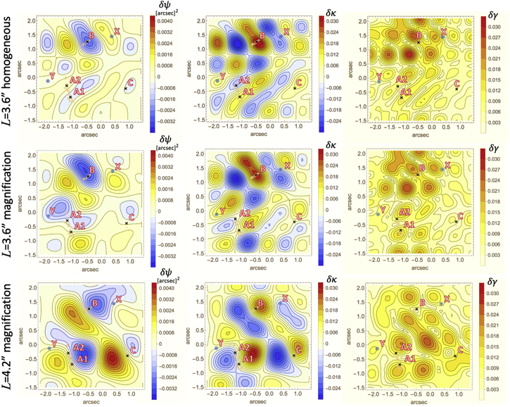
Figure 20. Contour maps of perturbations (36 modes) in Type A models best-fitted to the ALMA data, MIR flux ratios, and VLBA positions of a core component q. The plotted maps show the potential perturbation δ
ψ, convergence perturbation δ
κ, and shear perturbation δ
γ reconstructed with L = 36 and the homogeneous weighting (top column), L = 36 and the magnification weighting (middle column), L = 42 and the magnification weighting (bottom column). Light brown curves denote the boundaries of regions in which the signals are larger than 3σ. The centers of the square region are (−0.4, 0.3) (top), (−0.4, 0.3) (middle), and (−0.7, 0.3), (bottom). The coordinates are J2000 centered at the centroid of the primary lensing galaxy G. The slight difference between the best-fitted potential wells around A1, A2, and B images of the quasar core reconstructed with L = 36 and the magnification weighting (middle left) and that with L = 42 and the magnification weighting (bottom left) may be due to the slight difference in the angular scales of the Fourier modes (see also Figure 24).
Download figure:
Standard image High-resolution imageOur method can probe both the potential perturbation due to subhalos and LOS structures and distortion in the potential of the primary lens. Since the effect is degenerate with that of low-frequency potential perturbation due to subhalos and LOS structures, extracting only the distortion in the potential of the primary lens is difficult. Although it is somewhat ad hoc to determine the range of the "low" frequency affected by the primary lens, we adopted the lowest 6 modes with angular wavelength of 2'' ∼ 7'' as the "low-frequency" modes.
18
As shown in Figure 21, The convergence perturbation δ
κ due to the low-frequency modes is less than 0.002, corresponding to ∼0.4% of the background convergence of κ ∼ 0.5 in the effective Einstein radius. This result is expected, as low-frequency modes whose fluctuation scales are larger than the effective Einstein radius of the primary lens cannot perturb quadruple images independently. Thus, it is likely that our results for intermediate- and high-frequency modes are not very sensitive to the selected low-frequency modes (including deviation from SIE), which are partly associated with the potential of the primary lens. However, note that our result cannot exclude the possibility of contribution from very small angular scale modes <10, which we did not take into account.

Figure 21. Contour maps of low-frequency modes of the best-fitted convergence perturbations for the three Type A models shown in Figure 20. The plotted maps show the lowest mode (monopole; left), the sum of the second- and third-lowest two modes (dipole; middle), and the sum of the fourth- to sixth-lowest three modes (quadrupole; right). The symbols are the same as in Figure 20.
Download figure:
Standard image High-resolution imageWe also studied perturbed Type B models in which object Y is modeled by an SIE at a redshift zY = 0.661 in the smooth model (Figure 22). We found that the ratio of the difference of convergence contribution δ κ between A2 and B to A1 and B as (δ κ(A2) − δ κ(B))/(δ κ(A1) − δ κ(B)) = 2.8. The value is close to the ratio of the differential extinction of A2 to that of A1, ΔAV (A2)/ΔAV (A1) ≈ 3.4 (Inoue et al. 2017). Therefore, the large difference in the differential extinction of A2 relative to A1 can be naturally explained by our model if the convergence is proportional to the dust column density. Owing to the presence of small clumps in the vicinity of B and A1, the perturbed Type B models fit the MIR flux ratios better than the unperturbed background Type B model. Compared with the perturbed Type A models, the perturbed Type B models fit the VLBA positions of jet components much better (see Table 4). In Figure 23, we show the best-fitted convergence perturbations in the Type B models. One can visually confirm that the fluctuation patterns are similar to those in Type A models with the same parameters (see Figure 20). This suggests that the small-scale potential fluctuations are independent of the presence or absence of object Y.

Figure 22. Convergence of object Y (left) and caustics overlaid with critical curves in a perturbed Type B model in which object Y is explicitly modeled (right). The left panel shows a contour map of the convergence of a modeled object Y in the background Type B model. Green curves denote the boundary inside which the signal is >3σ. The right panel shows the caustics, cuts (black), and critical curves (red) in a perturbed Type B model with the magnification weight and L = 36. The red "X" symbols are the best-fitted positions of q in the lens plane, and the green "X" is the best-fitted position of q in the source plane. Blue circled dots are the centroid of object X and the position of the peak intensity of object Y.
Download figure:
Standard image High-resolution image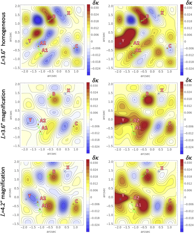
Figure 23. Contour maps of convergence perturbations δ
κ (36 modes) in Type B models in which object Y is explicitly modeled. The left row shows the convergence perturbations in which the contribution from object Y is subtracted. The right row represents the total convergence perturbations (object Y plus Fourier modes). The model was obtained with the source plane fits with L = 36 and the homogeneous weighting (top column), L = 36 and the magnification weighting (middle column), L = 42 and the homogeneous weighting (bottom column). Green curves denote the boundaries of regions in which the signals are larger than 3σ. The centers of the square region that determines the Dirichlet boundary condition are (−0.4, 0.3) (top), (−0.4, 0.3) (middle), and (−0.7, 0.3), (bottom). The coordinates are J2000 centered at the centroid of the primary lensing galaxy G.
Download figure:
Standard image High-resolution imageTo estimate the lensing power spectra toward MG J0414+0534, we used the homogeneous weighting, which was observed to be more suitable than the magnification weighting (Section 5.4). Similar to our mock analysis, the constant β was chosen to satisfy χ2/dof = 2.8 in the initial model without any perturbation. The 1σ errors of the powers were calculated using random Gaussian potentials that give Δχ ≤ 1 with the smoothing term Rs
/dof smaller than that for the best-fitted model. We used the two models (36 modes with L = 36 and L = 42) to estimate the lensing power spectra. Table 5 shows the lensing power spectra obtained from the 22 intermediate-frequency modes as was calculated in the mock analysis. The lensing power spectra of potential perturbation Δψ and astrometric shift perturbation Δα did not depend much on the side length L. In contrast, the convergence perturbations Δψ showed a weak dependence on L: a model with smaller angular scale has a slightly larger convergence perturbation. This tendency was observed in the lensing power spectra with much smaller bins (see Figure 24). Modes with smaller angular scales have a larger power. This tendency is more apparent for convergence perturbation than astrometric shift and potential perturbations. On the smallest angular scale, the difference in powers of Type A and those of B models becomes smaller. This result suggests that the lensing powers on the smallest angular scale obtained from the seven high-frequency modes are not so sensitive to the details of object Y. Therefore, we adopt the lensing powers on the smallest angular scale as the robust ones.

Figure 24. Lensing power spectra for potential (left), astrometric shift (middle), and convergence (right) perturbations for small bins. The measured values were obtained from the ALMA image, the MIR flux ratios, the HST positions of galaxies, and the VLBA positions of lensed images of a core component q. Blue (red) vertical and horizontal bars centered at filled diamonds show ∼1σ errors in the square root of power and the bin range of angular wavenumber l used for a Type A model obtained with the homogeneous weighting and L = 42 (L = 36), respectively. Blue (red) horizontal bars centered at empty diamonds show the bin range of angular wavenumber l and the best-fitted values for a Type B model obtained with the homogeneous weighting and L = 42 (L = 36), respectively. The power spectra at the smallest, intermediate, and largest angular bins were obtained from seven low-to-intermediate-frequency modes, 11 intermediate-to-high-frequency modes, and seven high-frequency modes. The highest one ((m, n) = (6, 6)) was not included (see Figure 9). Note that the errors in the three (potential, shift, and convergence) lensing power spectra are not independent as they are given by common Fourier modes with an angular scale of 360°/l.
Download figure:
Standard image High-resolution imageTable 5. Model Parameters and the Lensing Power Spectra Obtained from the 22 Intermediate-frequency Modes
| Type | Weighting | N2 | L | l[105] | δ θ | Δκ | χ2/dof | Rs /dof | dof | ||
|---|---|---|---|---|---|---|---|---|---|---|---|
| A | hom. | 36 | 36 | 8.6 ± 2.6 | 0.00070 ± 0.00004 | 0.0033 ± 0.0002 | 0.0079 ± 0.0005 | 1.2 | 0.12 | 18 | |
| A | hom. | 36 | 42 | 7.4 ± 2.2 | 0.00072 ± 0.00003 | 0.0030 ± 0.0002 | 0.0066 ± 0.0003 | 1.2 | 0.12 | 18 |


Note. They were obtained from the 22 intermediate-frequency modes, which are a subset of the 36 modes that were best-fitted to the ALMA data, MIR flux ratios, HST positions of galaxies, and VLBA positions of a jet component q. N2 is the number of mode functions. L is the side length of a square at which the Dirichlet condition is imposed. l is the angular wavenumber in degrees, and δ θ is the corresponding angular wavelength. To obtain de-lensed images, the homogeneous weighting was used.
Download table as: ASCIITypeset image
We summarize our results obtained from the source plane fit to the ALMA images as follows:
- 1.Using a discrete Fourier expansion of potential perturbation δ ψ, we were able to fit the VLBA positions of lensed images of a radio core, HST positions of the centroids of the primary lensing galaxy G and object X (object Y), peak-subtracted ALMA continuum image at 340 GHz, and MIR flux ratios observed with the Subaru and Keck telescopes. Using the obtained model parameters, we were able to fit the VLBA positions of lensed images of radio-jet components using the traditional lens plane fit without changing the model parameters.
- 2.The de-lensed source images show a bright spot centered at a radio core with a bipolar structure in the vicinity of the VLBA jet components.
- 3.The best-fitted models show a complex mass distribution with four clumps near the quadruple images. One clump near image A2 may be associated with object Y. The detailed structure of the mass distribution depends on the choice of assumed model parameters that were fixed in fitting.
- 4.The contribution to convergence from low-frequency modes is less than ∼0.4% of the background value.
- 5.The range of measured convergence power within 1σ of the mean values at the two smallest angular scales l = (1.11 ± 0.07) × 106 and l = (1.30 ± 0.08) × 106 was Δκ = 0.021–0.028. The mean angular scale l ∼ 1.2 × 10⁶ of the two measurements corresponds to the effective Einstein radius bG ∼ 11 of G. The power is significantly larger than those on larger angular scales >11. The ranges of measured astrometric shift and potential powers within 1σ of the two angular scales were Δα
= 7–9 mas and Δψ
= 1.2–1.6 mas2, respectively. The measured lensing powers at l ∼ 1.2 × 10⁶ were not so sensitive to the presence or absence of object Y.
6.3. Lens Plane Fit to ALMA Visibilities
As we have discussed, the effects of systematic errors due to limited sample of visibility data are significantly reduced in our partially nonparametric model fitting. However, residuals of systematic errors caused by the CLEAN deconvolution process or phase corruption may still affect the fitted models significantly. Therefore, we check one of our best-fitted model (Type A) using χ2 fit in the visibility plane (Hezaveh et al. 2013, 2016b; Rybak et al. 2015; Spilker et al. 2016; Maresca et al. 2022). Direct fitting to the visibility data obtained by our Cycle 2 and 4 observations can test whether the observed astrometric shifts are due to perturbation by LOS structures/subhalos or systematic errors caused by side lobes and phase corruption.
Since our fitting formalism cannot determine the absolute fluxes of lensed images, we parameterize the overall amplitudes of the best-fitted point sources (cores p, q) and extended sources (jets r,s and dust) in the lens plane by multiplying constants a and b to the pre-fitted model visibilities of point and extended sources, respectively. In what follows, we use a Type A model that was fitted to the ALMA data with the magnification weighting (36 modes and L = 36). We describe the detailed procedure of fitting visibilities to the ALMA data in Appendix
As described in Section 6.2, perturbation by LOS structures/subhalos produces thin tangential arcs across a critical line. Therefore, it is likely that such a perturbation preserves the radial structure of extended source visibility components (Figure 34). Moreover, the amplitude of point-source visibilities is invariant with respect to rotation in the visibility plane. Thus, we consider that grids defined in the polar coordinates are suitable to compress the data to analyze the effects of potential perturbation efficiently.
As one can see in Figure 25, the ALMA visibilities averaged with polar grids with azimuthal separation δ θ = 90° are dominated by errors at uv distance larger than ∼10,000 m that corresponds to the size of the synthesized beam. The extended components contribute to the visibilities more than the point-source components at distances smaller than ∼800 m, whereas the point-source components dominate the signal at distances larger than ∼800 m. Although the amplitudes of the total fitted model visibilities are comparable to the observed ones at distances ∼400–5000 m, we observe a slight excess in model visibilities at small distances ≲400 m possibly due to systematics in our CLEAN deconvolution process. Improvement in fitting with respect to no (null) model is more conspicuous for larger angular separations δ θ in which each grid has a larger number of samples (Figure 26). If δ θ is too small, much of the information of phase is lost, leading to a worse fit.


Figure 25. Comparison between observed and model (Type A) visibilities. The blue dots show the amplitude of visibilities on circular grids observed at 335.3 GHz vs. the uv distance . The radial separation of adjacent grids is 100 m, and the azimuthal separation is δ θ = 90°. The green, orange, and red curves show best-fitted Type A model visibilities at v = 0 m for the total, extended source, point-source components, respectively.

Download figure:
Standard image High-resolution image
Figure 26. Improvement in fitting with respect to no (null) model. The red filled circles show the reduced χ2 in a perturbed Type A model divided by that in no (null) model. δ θ is the angular separation between the centers of adjacent grids.
Download figure:
Standard image High-resolution imageFor 1° ≲ δ θ ≲ 90°, our visibility fitting showed that the perturbed model fits the ALMA data better than the corresponding unperturbed smooth model (Figure 27). We found that the optimal value of azimuthal separation that gives the best fit is δ θ = 10°. This result suggests that the improvement by including Fourier modes of potential perturbation is not caused by systematics due to side lobes and phase corruption. We also found that the improvement is caused by both the extended and point-source components. In order to have the evidence of improvement due to the extended source components, we fitted model visibilities in which the point-source flux ratio of A1 to A2 is artificially fixed to be unity while the extended source components were intact. If the improvement is not caused by extended components, then we can expect that the model visibilities will not show any improvements. However, as shown in Figure 27, we found that the fit was improved to some extent. Therefore, we conclude that the fit to the extended source components was indeed improved.

Figure 27. Comparison between perturbed and unperturbed Type A models. The red boxes and the blue stars show the reduced χ2 for the perturbed and unperturbed background Type A models, respectively. The green filled circles show the reduced χ2 for the perturbed Type A model in which the point-source flux ratios of A1–A2 are artificially fixed to be unity. δ θ is the angular separation between the centers of adjacent grids.
Download figure:
Standard image High-resolution imageAt δ θ = 10°, the coefficients of the point-source component and extended source component in the perturbed model were a = 1.8 ± 1.5 mJy and b = 0.42 ± 0.39. At δ θ = 90°, the corresponding values were a = 1.8 ± 0.8 mJy and b = 0.44 ± 0.19. The errors were obtained from a condition Δχ2/dof < 1. Thus the best-fitted values correspond to ∼20% and ∼60% decrease in overall amplitude with respect to the originally modeled intensity distribution of the point-source component and extended source component, respectively. The decrease in a is not statistically significant, but the significance of a decrease in b is at the ∼3σ level.
As we have seen in Section 5.2, our CLEAN deconvolution process gave a systematic boost in overall amplitudes of flux on large angular scales. Therefore, it can affect the model fit on large angular scales ≳07 (corresponding to a distance of ∼400 m). However, on small angular scales, especially for signals with large S/N, such systematic effects are expected to be small. The improvement of χ2 fit due to the extended source components implies that the perturbation effect caused by LOS structures and subhalos is limited to intensity fluctuations on relatively small angular scales ≲07. The size of the image residual in the lens plane (Figure 19) in Section 6.2 supports this interpretation.
Thus, we conclude that our results in visibility fitting and mock analysis suggest that observed astrometric shifts are due to perturbation by LOS structures/subhalos rather than systematic errors caused by side lobes and phase corruption.
6.4. Lens Plane Fit to VLBA Positions
Based on the above discussions, the reconstructed potentials in the lens plane exhibit some differences depending on the choice of the center and side length L of a square at which the Dirichlet boundary condition is imposed. In order to scrutinize the effect of perturbation, particularly in the vicinity of object Y, we also performed a χ2 fitting in the lens plane. We fitted the model to the positions of VLBA jet components p, q, r, and s, centroid of G and object X, and the MIR flux ratios of quadruple images with adjusting coefficients of the 22 intermediate-frequency Fourier modes and translation.
19
The positional errors are assumed to be 2 mas for q, 5 mas for p, r, s, and G, and 01 for X. The number of observed parameters is 4 × 2 × 4 + 2 × 2 + 3 = 39, and the number of fitting parameters is 22 + 2 + 8 = 32. We did not consider rotation of the potential.
If we conduct χ2 fitting for the positions, significant discontinuity in the potential perturbation may occur at places farther from the position of lensed jet components, as the size of jets are much smaller than the lensed arc observed in the ALMA image. To avoid such discontinuity, we imposed an additional constraint on the smoothness of perturbation. To do so, we minimized χ2 for the positions of G, X, and the VLBA jet components and MIR flux ratios plus the smoothing term Rs
defined in Equation (10). We fixed the smoothing parameters δψ0, δα0, and δκ0 to be the same or slightly smaller values obtained from the best-fitted models with the magnification weighting with L = 36 and N2 = 36 modes. To test the smoothing effect, we considered two types of χ2 fitting: with and without constraint on the smoothness of perturbation.
As shown in Table 6, the rms perturbations , ,
20
for fitting without constraint on smoothness are significantly larger than those for fitting with the constraint. Our results indicate that reconstructing the potential beyond the region of jet components is difficult if constraint on smoothness is not taken into account. The fit is slightly better for the model with L = 36 than that with L = 42. The obtained rms perturbations in the model with L = 36 and constraint on smoothness agree with those in the corresponding model with 36 Fourier modes obtained from the previous fits based on the ALMA image within 35%. Moreover, as shown in Figure 28, the fit to the VLBA positions of jet components p, q, and r in images A1 and A2 noticeably improved compared with the previous fit in the source plane using the ALMA data dominantly. Therefore, the obtained model may be significantly better in describing the perturbation in the vicinity of A2. As shown in Figure 29, the feature of potential perturbation δ
ψ is similar to that obtained with L = 36, N2 = 36 modes, and the magnification weighting (Figure 20).


Figure 28. The best-fitted VLBA positions of four jet components in the lens plane using the MIR flux ratios, HST positions of galaxies, and smoothing parameters that were used to fit the ALMA data. For the fitting, a Type A smooth model was used, and an additional 22 intermediate-frequency modes were adjusted with smoothing constraints . The red symbols represent the VLBA positions of p, q, r, and s observed at 5 GHz as in Figure 14, and circles indicate their 1σ errors. The black "X" symbols represent the best-fitted positions in a model with L = 36. The coordinates are J2000 centered at the centroid of the primary lensing galaxy G.

Download figure:
Standard image High-resolution image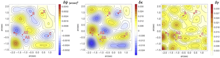
Figure 29. Contour maps of the best-fitted perturbations obtained from the MIR flux ratios, HST positions of galaxies, VLBA positions of four jet components p, q, r, and s, and smoothing parameters that were used to fit the ALMA data. For the fitting, a Type A smooth model was used, and an additional 22 intermediate-frequency modes were adjusted with smoothing constraints. The plotted maps show the potential perturbation δ
ψ, convergence perturbation δ
κ, and shear perturbation δ
γ reconstructed with L = 36. The gray curves denote the boundaries of regions in which signals are larger than 3σ. The red "X" symbols denote the positions of lensed jet component q. The centers of the square region are (−0.4, 0.3). The coordinates are J2000 centered at the centroid of the primary lensing galaxy G.
Download figure:
Standard image High-resolution imageTable 6. Parameters, Minimized χ2, Flux Ratios (Estimated at the Fitted Positions of q), and rms Perturbations in Type A Models Best Fitted to the MIR Flux Ratios, the HST Positions of Galaxies, and the VLBA Positions of Four Jet Components p, q, r, and s
| L | δ ψ0 | δ α0 | δ κ0 | χ2/dof | dof | A2/A1 | B/A1 | C/A1 | |||||||
|---|---|---|---|---|---|---|---|---|---|---|---|---|---|---|---|
| 3.6 | 0.0014 | 0.0053 | 0.0090 | 2.0 | 7 | 0.916 | 0.355 | 0.157 | 0.29 | 1.13 | 0.06 | 0.47 | 0.00097 | 0.0041 | 0.0092 |
| 3.6 | ∞ | ∞ | ∞ | 0.65 | 7 | 0.920 | 0.345 | 0.151 | 0.10 | 0.30 | 0.06 | 0.19 | 0.0031 | 0.0144 | 0.0346 |
| 4.2 | 0.00082 | 0.0051 | 0.0048 | 2.1 | 7 | 0.918 | 0.355 | 0.158 | 0.33 | 1.22 | 0.06 | 0.44 | 0.0011 | 0.0042 | 0.0084 |
| 4.2 | ∞ | ∞ | ∞ | 0.99 | 7 | 0.915 | 0.355 | 0.132 | 0.095 | 0.676 | 0.06 | 0.16 | 0.0028 | 0.0113 | 0.0238 |


Note. Only the 22 intermediate-frequency modes with translation were used for fitting. The parameters in the smooth model were fixed except for the position of an SIE+ES. L is the side length of a square at which the Dirichlet boundary condition is imposed. δ ψ0, δ α0, and δ κ0 are smoothing parameters that control the rms values defined in the square region. χ2 is the sum of for the MIR flux ratios, for the HST position of X, for the HST position of G, for the VLBA positions of four jet components. The rms perturbations , , and on the square region were obtained from the coefficients for the best-fitted 22 Fourier modes.


Download table as: ASCIITypeset image
Interestingly, the best-fitted convergence perturbation δ
κ indicates the presence of a clump in the vicinity of object Y as well as three clumps in the vicinity of image A1, B, and C. The distance between the local peak in the convergence and object Y is ∼03, which is smaller than the smallest fluctuation scale ∼09 of the fitted Fourier mode functions. Compared with the previous model in Inoue et al. (2017), the shape of the clump in the vicinity of Y is rounder. In the best-fitted models, a pair of clumps in the vicinity of B and a pair of clumps in the vicinity of A2 cause a shear perturbation δ
γ at A2 and B, respectively. They probably result in an improvement in the fit to the MIR flux ratios and VLBA positions of jet components. Our results indicate that potential perturbations consisting of several halos are more realistic and robust compared with perturbations consisting of only one halo.
6.5. Object Y
A faint continuum emission with a flux of 0.2–0.3 mJy at (R.A., decl.) = , in the north east of A2, was first reported by Inoue et al. (2017). We called it object Y. Using the same ALMA Cycle 2 data, Stacey & McKean (2018) pointed out that the emission disappears after self-calibration. To check the result, we added the data of our Cycle 4 (high-resolution) observations to the Cycle 2 (low resolution) data. For each data set of Cycle 2 and 4 data, we subtracted off the components of line emission and carried out phase-only self-calibration. Then we combined both of the data sets to obtain CLEANed images with various robust parameters. As shown in Table 7, with robust = 0, 0.5, we detected a faint emission with a peak flux density of 81.8, 114.5 μJy beam−1 at the position of object Y. The statistical significances were 3.6σ, 3.8σ. To increase S/N, we also carried out imaging with robust = 0 using the full-band data (self-calibrated line-free and line channels) and detected faint emission with a peak flux density of 84.2 μJy beam−1 at the position of object Y. The statistical significance is 3.7σ. Although the significances are not sufficiently high, as shown in Figure 30, the signals seem to be stable. In contrast, other faint spots with intensity <3.5σ are not stable. Their peak flux depends on the selected robust parameters and frequency. Note that the significance of object Y decreased to <3.0σ for the natural weighting. Thus, we cannot conclude the significance of the object Y.


Figure 30. ALMA images of object Y. The plotted black curves are contours of intensity with 3.5σ for line subtracted images with robust = 0 (left), robust = 0.5 (middle), and a full-band image with robust = 0 (right) overlaid with the best-fit convergence perturbation δ
κ obtained from the MIR flux ratios, HST positions of galaxies, VLBA positions of four jet components p, q, r, and s. The reconstruction was conducted with L = 36 and the smoothing parameters that were used to fit the ALMA data.
Download figure:
Standard image High-resolution imageTable 7. Flux of Object Y Measured in CLEANed Images
| Line-free | Line-free | Full-band | |
|---|---|---|---|
| Robust | 0.5 | 0 | 0 |
| rms errors [μJy beam−1] | 22.9 | 30.4 | 22.6 |
| Peak flux [μJy beam−1] | 81.8 | 114.5 | 84.2 |
| S/N [σ] at peak | 3.6 | 3.8 | 3.7 |
| Flux (>2σ) [μJy] | 36 | 79 | 63 |
| Peak ΔR.A. (J2000) | −1865 | −1866 | −1865 |
| Peak Δdecl. (J2000) | −0116 | −0116 | −0118 |
Download table as: ASCIITypeset image
In order to verify the weak emission from object Y, we performed visibility fitting. We used a Type A model that was best fitted to the ALMA, HST, Subaru, and VLBA data using the magnification weighting with L = 36. We added a Gaussian component at (−1865, − 0116)
21
in the J2000 coordinates in which the centroid of galaxy G is at (0,0). In the fitting, the flux of the Gaussian component was used as a free parameter as well as a and b that control the overall amplitudes of the pointlike and extended sources, but the position of the Gaussian source was fixed at the central position of object Y. The distance between object Y and the phase center (in the vicinity of q in A1) is , the corresponding baseline scale at ∼340 GHz is ∼40 m. The scale of the synthesized beam is 003, which corresponds to the baseline scale of ∼1500 m. Therefore, in order to retain the phase information of object Y, we needed to restrict the azimuthal separation of polar grids to . We plotted our result in Figure 31. The fitted flux values were 40–400 μJy and always positive. We also fitted our model to the full-band visibility data. Our fitting result showed that the fitting to the full-band data is worse than the line-free data (left panel in Figure 32). Since we did not include line components in the model, the result is not surprising. Interestingly, compared to the line-free data, the full-band data showed an enhanced improvement in fitting compared to the model without object Y (right in Figure 32). Since the S/N of emission from object Y is expected to be higher in the full-band data, the result is again not surprising. Thus, we were not able to exclude the possibility that the weak continuum emission is associated with object Y rather than systematic errors.


Figure 31. Result of visibility fitting in which object Y is modeled by a Gaussian source. The blue line shows the best-fitted flux of object Y. δ
θ is the angular separation between the centers of adjacent grids. We used a perturbed Type A model with the magnification weighting and L = 36. In the fitting, only the line-free visibility data were used.
Download figure:
Standard image High-resolution image
Figure 32. Comparison of results of visibility fitting. The left and right figures show the reduced χ2 for models with object Y and the difference in the reduced χ2 between models with and without object Y (Δχ2 ≡ χ2(with Y) − χ2(without Y)), respectively. In each figure, the blue dashed and red lines correspond to the results fitted to the line-free and full-band visibility data, respectively.
Download figure:
Standard image High-resolution imageHowever, it should be noted that the origin of the weak emission is still not confirmed. In order to confirm the weak emission, we need to carry out new ALMA observations at frequency ≳340 GHz with angular resolution ≲01 with sensitivity better than ∼10 μJy beam−1.
7. Consistency with CDM Model
As shown in Section 6.2, the range of measured amplitude of convergence perturbation within 1σ at an angular scale of ∼11 (l ∼ 1.2 × 10⁶) was Δκ
= 0.021–0.028. This result was obtained using the seven high-frequency modes. Assuming that the seven modes are independent each other and obey a Gaussian distribution, the cosmic variance is at most . Therefore, the measured values including the error due to the cosmic variance are Δκ
= 0.015–0.032. Assuming a constant convergence power over a range of angular wavenumber Δl ∼ l, the obtained value seems to be at odds with theoretical prediction (Inoue 2016) at quadruple images with separation angle of in which only CDM subhalos in the primary lensing galaxy are taken into account. If we add contribution from LOS structures to that from CDM subhalos, the CDM prediction yields δ
κrms = 0.018 ± 0.007 (Inoue 2016) assuming that object X is not residing in the primary lens plane (Takahashi & Inoue 2014) and baryons in the primary lensing galaxy do not significantly affect the lensed image (Hsueh et al. 2018). Therefore, our result is consistent with the CDM prediction. Although, we cannot deny the possibility of chance alignment of subhalos with the quadruple images, our results support the idea that anomalies in the flux ratios and astrometric shifts in galaxy-scale quadruple lenses at zs > 2 are primarily caused by LOS structures rather than subhalos. In other words, our results are consistent with the predicted abundance of intergalactic halos in CDM models on ∼10 kpc scale.


Expressing convergence perturbations in terms of mass scale might be helpful to galactic astronomers. The mean of the measured convergence perturbation Δκ = 0.025 for a source redshift zs = 2.639 and a lens redshift zl = 0.9584 is equal to if the total mass resides at zl (Takahashi & Inoue 2014). Assuming that the convergence power is proportional to the proper length to the source (Inoue & Takahashi 2012), our result suggests a convergence power of 5 × 10⁸ M⊙ per 5 kpc scale for a source redshift zs = 0.982 and a lens redshift zl = 0.28, which is slightly larger than the recent upper bound of convergence power 3 × 10⁸ M⊙ for a proper length scale of 3 kpc obtained from the HST observations of SDSS J0252+0039 (Bayer et al. 2023). Taking into account the cosmic variance, our result is consistent with the HST result.

8. Conclusion and Discussion
We obtained the first lower and upper bounds of the lensing power spectra on ∼10 kpc (on the primary lens plane) scale toward MG J0414+0534 using our new partially nonparametric method. Based on Type A models, the range of measured convergence, astrometric shift, and potential powers within 1σ at an angular scale of ∼11 (corresponding to an angular wavenumber a number of waves per 360° of l ∼ 1.2 × 10⁶ or ∼9 kpc in the primary lens plane) were Δκ
= 0.021–0.028, Δα
= 7–9 mas, and Δψ
= 1.2–1.6 mas2, respectively. Our simple estimate suggests that the obtained values are consistent with the CDM prediction. To measure the power spectra, we conducted ALMA observations with high angular resolution 002–004 toward the anomalous quadruply lensed quasar MG J 0414+0534 at zs = 2.639. We also used the MIR ratios of quadruple images, VLBA positions of jet components, and HST positions of galaxies.
In a mock analysis, we observed that the residual errors of measured power spectra for potential and astrometric shift perturbations are smaller than that for convergence perturbation. This result is expected, as interferometers such as VLBA and ALMA can measure astrometric shifts with small systematic errors. To date, astrometric weak lensing effect has been measured only in the near universe (Mondino et al. 2020). Our first measurement of power spectra with upper and lower bounds for potential and astrometric perturbations in the far universe creates a basis for constraining cosmological models with better accuracy.
Our method can directly measure lensing power spectra on certain angular scales and provides more accurate results than the previous methods based on only flux ratios or only astrometric shifts. To estimate the rms convergence perturbation from flux ratios of lensed images, we must assume the amplitudes of shear perturbation. For completely isotropic perturbations, the rms convergence perturbation is equal to the rms shear perturbation. Since the number of available fluxes that can be used to estimate convergence perturbation is limited, such an assumption would cause some errors (though not systematic) in each lens system. If we use only astrometric shifts to reconstruct the perturbation, our numerical analysis demonstrated that the convergence tends to become excessively large in regions beyond the lensed arcs in which the astrometric shifts are measured. Since astrometric shifts are related with the first spatial derivatives of the projected potential, not the second one, such a behavior can be naturally expected. Inclusion of ALMA data is essential, as it provides information for a radial profile of mass that cannot be obtained using VLBA observations. Using positions of jet components and extended dust emission on scales >1 kpc as well as MIR flux ratios, which are microlensing free, our multiwavelength method provides us with a very effective tool for probing matter fluctuations on scales ≲10 kpc in the universe.
Our method based on decomposition with discrete Fourier modes enables us to measure lensing power spectra directly from a single lensing system based on source plane χ2 + α evaluation. Note that noise cancellation due to synthesized multiple lensed images makes our method suitable for systems with extended images obtained from interferometers. Moreover, our method can be applied to systems with a source with a complex structure, as constraints on the source intensity are not stringent.
Our test using visibility plane fitting suggested that the improvement of fit achieved by our algorithm is not likely caused by systematics due to side lobes and phase corruption even if the overall intensity is not preserved by imaging using CLEAN. Gravitational perturbation causes tiny "arc-like" changes in the lens plane. Therefore, the effect of perturbation is very weak in the visibility plane as tiny arc-like structures are fast Fourier transformed to large arcs. On the other hand, the signal in the source plane is enhanced due to a linear combination of distant multiple images. Therefore, it is likely that our method has an advantage in detecting potential perturbation due to LOS structures/subhalos if properly applied to the lens system. Our visibility fitting method is useful for calibrating the absolute flux of pointlike and extended sources.
In our mock analysis, to obtain the lensing power spectra toward MG J 0414+0534, the homogeneous weighting seems to be more suitable than the magnification weighting. Since the magnification weighting puts large weights on very bright regions, the improvement in fitting is limited to regions with a large intensity. On the other hand, the homogeneous weighting treats multiple images equally. Therefore, we expect that it retains the information of fluctuations outside the bright regions, leading to a robust estimate of powers. However, in some systems, a certain "robust" weighting that lies in the middle of the both weighting may be optimal. We must further study this de-lensing problem using various lens systems.
In our algorithm, we included a term that controls the smoothness of perturbation beyond the lensed images to χ2. To verify such constraints, we may require one to assume that the lensing power spectra are sufficiently homogeneous inside the square region. Such an assumption is natural if the dominant contribution is from LOS structures. The cosmological principle states that there is no special direction in the universe. If the lensing power spectra are homogeneous, then the smoothness of potential, astrometric shift, and convergence due to LOS structures are determined by the lensing power spectra or equivalently the corresponding rms values in the lens plane to some extent. However, higher-order correlations such as bispectra and trispectra may be necessary for describing non-Gaussian and nonlinear perturbations. If the expected perturbation is strongly non-Gaussian, we may require one to consider more inhomogeneous, unsmooth potential perturbations. From our previous analysis based on N-body simulations, such effects seem insignificant if the positions of quadruply lensed images can be well fitted by a smooth potential such as an SIE. Our mock analysis in this paper also supports this result. Nevertheless, extension of our formalism to higher-order statistics is one of our next immediate scientific goal.
In our analysis, we neglected perturbations whose fluctuation scale is less than ∼1'' due to lack of S/N and angular resolution to resolve tiny distortion. We consider that such restriction is not a significant problem. First, our models using the source plane χ2 successfully fit the MIR flux ratios of lensed images, the VLBA positions of jets, and the HST positions of lensing galaxies simultaneously. In our formalism, the strength of astrometric shifts becomes larger for smaller angular wavenumbers. Therefore, even if the MIR flux ratios can be fit with a perturbation whose fluctuation scale is less than ∼1'', it would be difficult to simultaneously fit the VLBA positions of jets and the HST positions of lensing galaxies. Second, in CDM models, the convergence power spectrum moderately decreases as a function of the angular scale for ≲1'' (corresponding to a wavenumber k ≳ 100 h Mpc−1 at z ∼ 1; Inoue et al. 2015). Therefore, we expect that ∼1'' is the angular scale that contributes dominantly to the power.
The simulations conducted to date to estimate the nonlinear power spectra on small scales at redshifts z < 3 are for dark matter only. Inclusion of baryonic physics may enhance small-scale powers to some extent. Because of the uncertainty in baryonic physics, our results should be tested by future observations with improved S/N and angular resolution.
Acknowledgments
K.T.I. would like to thank Eiji Akiyama, Misato Fukagawa, Fumi Egusa, and Kazuya Saigo for their support on data reduction, Yuichi Higuchi for valuable discussion, and the anonymous referees for providing valuable comments, and acknowledge support from NAOJ ALMA Scientific grant No. 2018-07A, ALMA Japan Research Grant of NAOJ ALMA Project, NAOJ-ALMA-256, and JSPS KAKENHI grant No. 17H02868. S.M. is supported by the Ministry of Science and Technology (MoST) of Taiwan, MoST 103-2112-M-001-032-MY3, 106-2112-M-001-011, and 107-2119-M-001-020. K.N. is supported by JSPS KAKENHI grant No. 19K03937. This paper makes use of the following ALMA data: ADS/JAO.ALMA Nos. 2013.1.01110.S. and 2016.1.00281.S. ALMA is a partnership of ESO (representing its member states), NSF (USA), and NINS (Japan), together with NRC (Canada), MOST and ASIAA (Taiwan), and KASI (Republic of Korea), in cooperation with the Republic of Chile. The Joint ALMA Observatory is operated by ESO, AUI/NRAO, and NAOJ.
Data Availability
The ALMA data used in this work can be downloaded from the ALMA archive: https://almascience.nao.ac.jp/aq/. The corresponding project codes are ADS/JAO.ALMA Nos. 2013.1.01110.S. and 2016.1.00281.S.
Appendix A: Lensing Power Spectra
Using discrete Fourier modes, a real-valued scalar perturbation δ X( θ ) of X defined on a square with an area of 22 in the real space θ can be decomposed as


where is a Fourier coefficient for a wavevector k , which can be expressed in terms of a set of nonnegative integers (n1, n2) as


The power spectrum PX (k) of an ensemble of perturbations δ X is defined as

where 〈〉 is an ensemble average for a fixed k = ∣ k ∣. The dimensionless power spectrum as a function of k is defined as


We express the square root of the spectrum as . From an observed image, we can measure the estimated dimensionless power spectrum as


where 〈〉angle denotes an ensemble average over various directions of wavevectors that have and , where n1 and n2 are the mode numbers that give . A lensing power spectrum is defined as a dimensionless power spectrum in which X is either a projected gravitational potential ψ, strength of astrometric shift α or convergence κ. The ensemble average of squared perturbation of X for a range of angular wavenumbers k − Δk/2 < k < k + Δk/2 can be estimated as


where ∣Δk∣ ≪ k. In terms of real Fourier coefficients , the right-hand side of (A6) must be divided by 1/4 (see Appendix B),


The angular wavenumber can be also expressed as the number of waves per 360° as l = 180 k/π. For an angular wavelength of δ θ in units of arcseconds, the corresponding angular wavenumber is

Appendix B: Two-dimensional Real and Complex Fourier Series
Since we do not consider any zero modes, a real scalar function f( r ) defined in a region and can be decomposed as a real Fourier series as


where m and n are natural numbers and .

Similarly, it can be decomposed as a complex Fourier series as

where and are nonzero integers. Since f is real, we have . Thus, we obtain


which results in

Appendix C: Procedure of Fitting Visibilities to the ALMA Data
In order to implement fast computation, we need to compress the observed visibilities in time and frequency domains. First, we averaged visibility data in each channel bin with an integration time of 60 s using CASA 6.4. Then the average distance between adjacent sampling points in the visibility plane was ≲10 m, which is much shorter than the minimum baseline ∼15 m that corresponds to an angular scale at ∼340 GHz, which is sufficeintly larger than the angular size of MG J0414+0534. Therefore, the data compression does not significantly affect visibility fitting in our ALMA data. Then, we concatenated Cycle 2 and Cycle 4 data and averaged line-free channels in each of four spectral windows (SPWs), which produced four visibility data sets centered at 335.3, 336.6, 346.7, and 349.5 GHz with ∼1.7 × 10⁵ elements. The four SPWs were numbered as s = 1, 2, 3, and 4 in ascending order. The effective bandwidths of the SPWs were 1–2 GHz, and the expected systematic reduction in the flux of a point source due to the bandwidth smearing effect in our setting (assuming a square bandpass and circular Gaussian beam taper) was ≲1%. Since the expected change in the fluxes of compact sources is ∼10%, the smearing effect is negligible.

In order to compare the modeled visibilities to the data, we need to estimate the rms noise. The CASA weight in the ALMA Measurement Set cannot be used as an estimated error in measured visibilities because the absolute values are not properly calibrated for some technical reason. 23 In our analysis, the standard deviation σsI of a visibility with an SPW number s and a sample number I in the visibility (u, v) plane was simply estimated as


In other words, the variance in the subtracted visibilities in a particular bin was assumed to be twice the true noise variance (Hezaveh et al. 2016b; Dye et al. 2018). To obtain the pre-fitted visibilities of the point-source components, we fitted p and q components in the VLBA data to the ALMA data, and we assumed that the flux ratios were given by the MIR values. The tentative absolute flux values of each component were specified by cq = 0.324 and cp = 0.626 (see Table 4). As the pre-fitted visibilities of the point-source components, we used the Fourier transformed Dirac delta functions of these components. The obtained visibilities were multiplied by a constant parameter a that has a dimension of janskys.
To obtain the pre-fitted visibilities of the extended-source components, we need to compute a matrix that consists of the extended source intensity at pixels in the lens plane. To do so, we used a PSF-subtracted ALMA image with the magnification weighting over a square region with a side length of 60 and a pixel size of 0005 (pixel number Nc
= 1200). Then, we padded zeros around the edge of the matrix (i.e., equivalent to adding a blank field) so that the dimension of the matrix becomes three times larger. The zero-padding significantly improves the accuracy of large-scale fluctuations in intensity. In order to perform the fast Fourier transform (FFT), we rearranged the matrix elements so that the center of the extended square region with a side length of 180 is shifted to the bottom-left corner. The rearrangement is equivalent to a swap between the first (second) and the third (fourth) quadrant. Second, we performed a two-dimensional FFT on the matrix data of the extended source components and rearranged the FFTed matrix as is done in the original matrix data (see Figure 33). We made a reflection in the R.A. direction and a translation by a half pixel size in the negative R.A. and decl. directions.
24
The obtained visibilities of the extended-source components (see Figure 34) were multiplied by a constant parameter b that has no dimensions.

Figure 33. A pre-fitted pixelized model image (left), the rearranged model image (center), and the FFTed image before rearrangement (right). The image size and the pixel size in the sky are and 0005, respectively. The model images with point- and extended-source components are shown only for illustrative purposes. In our analysis, pixelized images were used only for computing visibilities of extended source components, and zero-padding around the image was used to improve the accuracy of visibilities on large angular scales.

Download figure:
Standard image High-resolution image
Figure 34. The amplitudes (top column) and phases (bottom column) of visibilities in the (u, v) plane for the pre-fitted model shown in Figure 23. The visibilities (right row) are given by the sum of those of the extended source components (left row) and those of the point-source components (center row).
Download figure:
Standard image High-resolution imageFinally, a statistic (χ2 in the visibility plane) can be written as


where and are modeled complex visibilities of the point-source components and those of extended source components, respectively. It should be noted that the modeled complex visibilities were calculated using weights extracted from the observed ALMA Measurement Sets. We used the same sample (u, v) coordinates and weights of observed visibilities before averaging at grids.


We found that the obtained divided by the degrees of freedom (dof; i.e., reduced χ2) was almost equal to 1 even without taking into account model visibilities. This result suggests that the S/N of each visibility is so small that performing naive χ2 fitting is very difficult. We also tried to perform χ2 analysis using visibilities that have an apparent "high" S/N, but this resulted in biased results. Most visibilities with a "high" S/N actually have a systematically large error due to the low S/N. Therefore, restricting visibilities with apparently "high" S/Ns leads to a positive bias in the estimated amplitudes.

In order to circumvent the problem, we need to compress the visibility data in a certain way. In our analysis, we used visibilities that are averaged on grids (denoted by J) in the polar coordinates (r, θ) with a radial bin size of δ r = 100 m and an azimuthal size of δ θ in the visibility plane (u, v; Figure 35). The error variance of an averaged visibility at the Jth grid and an SPW number s was calculated as

where I(J) is a sample number within the Jth grid, and NJ is the total number of such sampled points. The averaged model complex visibilities on grids were calculated using CASA weights extracted from the observed ALMA Measurement Sets, which are proportional to the errors of visibilities. The selected (u, v) coordinates before averaging visibilities were the same as those used in our ALMA observations.

Figure 35. Distribution of grid centers. Each blue dot shows the center of a grid that contains sampled ALMA visibility data at 335.3 GHz. The radial and azimuthal angular separations of centers of adjacent grids are δ r = 100 m and δ θ = 10°, respectively.
Download figure:
Standard image High-resolution imageFootnotes
- 6
Anomalies in flux ratios can be caused by microlensing due to stars in the lensing galaxy (Zimmer et al. 2011). However, the effects of microlensing are negligible in MIR or radio observations due to the large size of source.
- 7
In ALMA Cycle 2, the position reference frame in Measurement Sets (storing data of visibilities and information of observation) were given as J2000. However, the actual position reference frame of the phase calibrators used in Cycle 2 was ICRS, which causes systematic errors of ∼0
01 in the positions. - 8
We did not include flexion (third derivative of potential) terms in describing potential fluctuations of massive objects located far from the lens (Okura et al. 2007; McCully et al. 2017; Fleury et al. 2021) as they can be considered as low-frequency Fourier modes. Similarly, we did not consider the third or fourth order multipoles m = 3 and m = 4 explicitly.
- 9
- 10
If a massive object resides in regions outside the lens plane of the primary lens, a rotational (magnetic) component of astrometric shift may not be negligible.
- 11
In the source plane, correlation between pixels due to side lobes is significantly suppressed as side lobe patterns do not correlate with the shape of lensed images.
- 12
Instead, we may impose the periodic boundary condition. However, in that case, we must consider a square with twice the side length.
- 13
If absolute magnification is excessively large, the second-order effect due to coupling between the perturbations on the parameters in the background and foreground cannot be neglected.
- 14
1σ errors are calculated by considering >106 sets of random Gaussian potentials that give Δχ ≤ 1 with the smoothing term smaller than that for the best-fitted model. The best-fitted potential was selected as the "center" of the random Gaussian potentials.
- 15
- 16
Although image A1 is slightly brighter than image A2, the angular separation between p and q in image A1 is far smaller than the separation in image A2 (Figure 15). That is why we chose A2 as the fiducial image.
- 17
If the fluctuation scale of intensity is smaller than the synthesized beam, the fit may become worse due to shrinking of the lensed image.
- 18
In the limit of L → ∞ , these lowest modes correspond to multipoles m = 0, 1, and 2 in the polar coordinates.
- 19
We conducted a similar analysis using the six high-frequency modes and the 22 modes, but the fit was worse.
- 20
For the model with L = 3
6 and N2 = 36 reconstructed with the magnification weight, we had . - 21
The position corresponds to the local peak in intensity in the CLEANed image obtained from the self-calibrated line-free components of our Cycle 2 and 4 data.
- 22
If we impose the Dirichlet boundary condition on a square with a side length of L, the corresponding area is A = 4L2 and .
- 23
https://casaguides.nrao.edu/index.php/DataWeightsAndCombination#Absolute_Accuracy_of_the_Data_Weights. We confirmed that the error values obtained from CASA weight were systematically smaller than the values obtained from the sample variance of the observed visibilities.
- 24
This translation is related to the difference between the fit convention that a pixel (Nc /2 + 1, Nc /2 + 1) is at the coordinate center (0, 0) and the image convention that (Nc /2 + 1, Nc /2 + 1) is at (pixelsize/2, pixelsize/2).


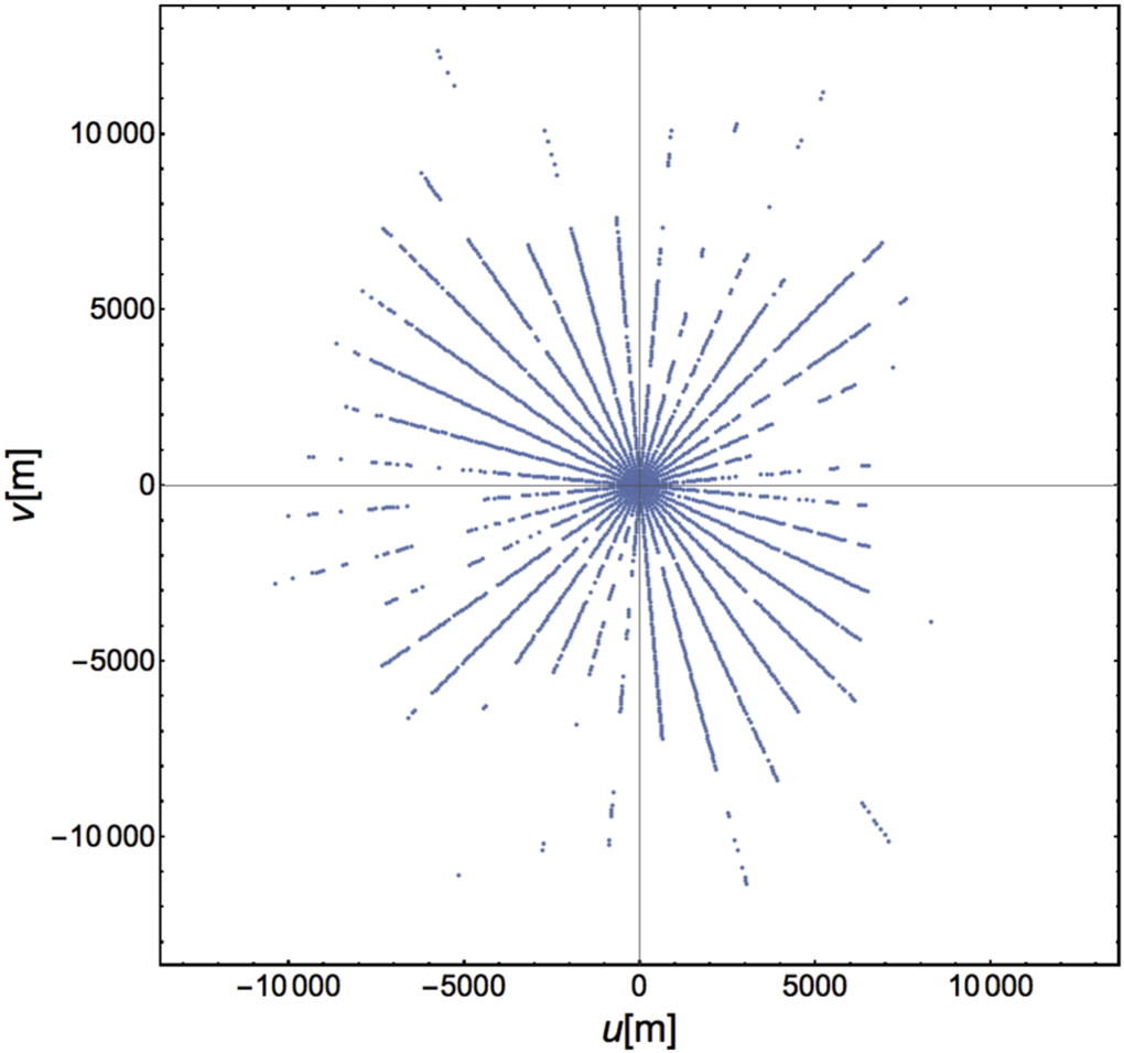