


Abstract
We present the first cosmological constraints derived from the analysis of the void size function. This work relies on the final Baryon Oscillation Spectroscopic Survey (BOSS) Data Release 12 (DR12) data set, a large spectroscopic galaxy catalog, ideal for the identification of cosmic voids. We extract a sample of voids from the distribution of galaxies, and we apply a cleaning procedure aimed at reaching high levels of purity and completeness. We model the void size function by means of an extension of the popular volume-conserving model, based on two additional nuisance parameters. Relying on mock catalogs specifically designed to reproduce the BOSS DR12 galaxy sample, we calibrate the extended size function model parameters and validate the methodology. We then apply a Bayesian analysis to constrain the Lambda cold dark matter (ΛCDM) model and one of its simplest extensions, featuring a constant dark energy equation of state parameter, w. Following a conservative approach, we put constraints on the total matter density parameter and the amplitude of density fluctuations, finding Ωm = 0.29 ± 0.06 and  . Testing the alternative scenario, we derive w = −1.1 ± 0.2, in agreement with the ΛCDM model. These results are independent and complementary to those derived from standard cosmological probes, opening up new ways to identify the origin of potential tensions in the current cosmological paradigm.
Export citation and abstract BibTeX RIS

Original content from this work may be used under the terms of the Creative Commons Attribution 4.0 licence. Any further distribution of this work must maintain attribution to the author(s) and the title of the work, journal citation and DOI.
1. Introduction
Over the past decade, cosmology has witnessed an unprecedented technological advancement prompting the release of a huge amount of data about our Universe. This has been made possible thanks to a massive experimental effort conducted by means of wide and deep-field surveys, complemented with the development of large and complex cosmological simulations. In this context, the study of cosmic voids, vast underdense regions of our Universe, began to provide its fundamental contribution in addressing fundamental questions in cosmology (see Pisani et al. 2019; Moresco et al. 2022, for a review).
With their large extent and unique low-density interior, voids indeed represent the ideal environment to study dark energy and modified gravity theories (Clampitt et al. 2013; Spolyar et al. 2013; Cai et al. 2015; Hamaus et al. 2015; Pisani et al. 2015a; Zivick et al. 2015; Achitouv 2016; Pollina et al. 2016; Sahlén et al. 2016; Falck et al. 2018; Sahlén & Silk 2018; Paillas et al. 2019; Perico et al. 2019; Verza et al. 2019; Contarini et al. 2021, 2022), as well as models including massive neutrinos (Massara et al. 2015; Banerjee & Dalal 2016; Kreisch et al. 2019, 2022; Sahlén 2019; Schuster et al. 2019; Contarini et al. 2021), primordial non-Gaussianities (Chan et al.2019) and phenomena beyond the standard model of particle physics (e.g., Reed et al. 2015; Yang et al. 2015; Baldi & Villaescusa-Navarro 2018; Lester & Bolejko 2021; Arcari et al. 2022).
The most straightforward analysis in this context is to count cosmic voids as a function of their size. This statistic is called the void size function. In recent years it has been explored in detail through cosmological simulations (e.g., Pisani et al. 2015a; Pollina et al. 2017; Contarini et al. 2019, 2021, 2022; Ronconi et al. 2019; Verza et al. 2019; Pelliciari et al. 2023) and more rarely with real survey catalogs (Nadathur 2016; Sahlén et al. 2016; Pollina et al. 2019). Another fundamental and extensively studied void statistic is the void-galaxy cross-correlation function, which represents an equivalent of the void density profile (Hamaus et al. 2014b; Schuster et al. 2023). It has been exploited for cosmological purposes by means of modeling the geometric and dynamic effects on the average void shape (Lavaux & Wandelt 2012; Pisani et al. 2014; Cai et al. 2016; Hamaus et al. 2016, 2017, 2020, 2022; Hawken et al. 2017, 2020; Achitouv 2019; Correa et al. 2019; Aubert et al. 2022; Nadathur et al. 2020, 2022; Correa et al. 2022; Woodfinden et al. 2022). Other notable and modern void analyses concern the weak lensing phenomenon (Clampitt & Jain 2015; Chantavat et al. 2016, 2017; Gruen et al. 2016; Cai et al. 2017; Sánchez et al. 2017b; Baker et al. 2018; Brouwer et al. 2018; Fang et al. 2019; Davies et al. 2021; Vielzeuf et al. 2021; Bonici et al. 2022), as well as the void autocorrelation function (Chan et al. 2014; Hamaus et al. 2014a, 2014c; Clampitt et al. 2016; Chuang et al. 2017; Kreisch et al. 2019; Voivodic et al. 2020), and the impact from voids on the integrated Sachs–Wolfe effect in the cosmic microwave background (Granett et al. 2008; Cai et al. 2014, 2017; Kovács 2018; Kovács et al. 2019, 2022b; Dong et al. 2021; Hang et al. 2021; Vielzeuf et al. 2021).
The various void statistics allow us to investigate the theoretical foundations of our Universe and test the current standard cosmological scenario, i.e., the Lambda cold dark matter (ΛCDM) model. Using real data catalogs to obtain effective cosmological constraints on the ΛCDM parameters, or to examine its main alternatives (see, e.g., Yoo & Watanabe2012; Joyce et al. 2016; Amendola et al. 2018, for a review), requires complete and statistically relevant void samples. For this reason, cosmic voids are usually analyzed in spectroscopic wide-field surveys (e.g., Sutter et al. 2012a; Hamaus et al. 2016; Nadathur 2016; Mao et al. 2017a; Hawken et al. 2020; Kovács et al. 2022a), covering large and possibly contiguous regions of the sky (see Sutter et al. 2014b, for tests on the impact of the survey mask on void statistics).
On the basis of this requirement, we here employed the final data release (Data Release 12, DR12) of the Baryon Oscillation Spectroscopic Survey (BOSS; Dawson et al. 2013), provided by the Sloan Digital Sky Survey (SDSS) III (Eisenstein et al. 2011). Thanks to its wide and contiguous sky area coverage, this galaxy catalog is indeed particularly suited to study cosmic voids. Mao et al. (2017b) explored the void sample extracted from the distribution of the BOSS DR12 galaxies and assessed its purity taking into account survey boundaries, masks, and radial selections. Then, assuming stacked voids to be spherically symmetric, Mao et al. (2017a) performed the Alcock–Paczynski test (Alcock & Paczynski 1979) to the same sample of voids in order to evaluate the matter content of the Universe, Ωm. Moreover, Hamaus et al. (2016) made use of BOSS data to study the joint effects of geometric and dynamic distortions on the stacked void-galaxy cross-correlation function, deriving precision-level constraints on Ωm and on the growth rate of structures. Other important works focusing on the study of voids from the SDSS have been conducted during recent years (e.g., Hoyle & Vogeley 2004; Pan et al. 2012; Sutter et al. 2012b, 2014b; Hamaus et al. 2017, 2020; Mao et al. 2017b; Nadathur et al. 2020; Aubert et al. 2022), but in none of these has the void size function been exploited as a cosmological probe.
In this paper, our goal is to measure and model the size function of BOSS DR12 voids to test the standard cosmological scenario. Since it offers cosmological constraints that are complementary to those of standard cosmological probes, this kind of analysis is extremely promising (Bayer et al. 2021; Contarini et al. 2022; Kreisch et al. 2022; Pelliciari et al. 2023). In particular, the negligible correlation between void counts and the main overdensity-based statistics (e.g., galaxy clustering and the halo mass function), together with the striking orthogonality of the corresponding growth of structure constraints (i.e., the Ωm–σ8 confidence contours), has revealed the utmost importance of modeling the void size function, in the perspective of combining its achievements with those of other cosmological probes.
The analysis that we present in this paper represents the first cosmological exploitation of the void size function as stand-alone probe (see however Sahlén et al. 2016, for the modeling of extreme-value void count statistics). With this pioneering work, we provide valuable cosmological constraints on the Ωm–σ8 parameter plane, and we test the standard ΛCDM scenario by analyzing its simplest alternative based on a constant dark energy equation of state.
The paper is organized as follows. In Section 2 we provide the theoretical foundations of the void size function model, and extend its standard theory to include observational effects and parameterize the galaxy bias contribution on the void radius. In Section 3 we describe the galaxy catalogs employed for the analysis, together with the procedure of void identification and cleaning. Moreover, we outline the details of the Bayesian analysis performed to test different cosmological scenarios, and we present the results of the void size function model calibration, attained through void mock catalogs. In Section 4 we apply the calibrated void size function model to the BOSS DR12 data and present the main outcome of the work. Finally, in Section 5 we draw our conclusions and discuss future applications of the analysis.
2. Theory
2.1. Void Size Function
The comoving number counts of voids as a function of their radius, i.e., the void size function, has been modeled from first principles by Sheth & van de Weygaert (2004). This model is developed within the framework of the excursion-set theory, with the same formalism adopted for the halo mass function (Press & Schechter 1974; Peacock & Heavens 1990; Bond et al. 1991; Cole 1991; Mo & White 1996). The multiplicity function, expressing in this case the volume fraction of the Universe occupied by cosmic voids in linear theory, 8 yields
with

where σm is the rms variance of the linear matter perturbations on a scale RL, while  and
and  are the two fundamental barriers of the model.
9
are the two fundamental barriers of the model.
9
The multiplicity function of Equation (1) assumes initial spherical density fluctuations to evolve according to linear theory over cosmic time. Therefore, to predict the number counts of observed voids of size R, we need to consider the nonlinear evolved density field. For this purpose, Jennings et al. (2013) modified the void size function model imposing the conservation of the volume occupied by voids during the transition from linearity to nonlinearity, which for this reason is called volume-conserving (hereafter, Vdn) model and is expressed as

The Vdn model successfully predicts the size function of cosmic voids identified in the total matter field (i.e., in the distribution of dark matter particles), provided that these voids are defined as spherical nonoverlapping spheres embedding a specific density contrast  (Jennings et al. 2013; Ronconi & Marulli 2017; Contarini et al. 2019; Ronconi et al. 2019). The threshold
  is the nonlinear counterpart of the quantity
  introduced in Equation (2), where the subscript "DM" specifies the requirement to be computed in the dark matter density field. To convert the nonlinear threshold into its linear counterpart and vice versa, we can make use of the fitting formula provided by Bernardeau (1994):

which features enhanced precision when applied to underdensities.
One of the observational effects to consider when computing the theoretical void size function is the so-called geometric distortions, which are caused by the assumption of a fiducial cosmology that may not coincide with the true one. Geometric distortions affect the observed void shape by introducing an anisotropy between the directions parallel and perpendicular to the line of sight. This distortion is commonly denoted as the Alcock & Paczynski (1979; AP) effect and can be modeled following the prescriptions by, e.g., Sánchez et al. (2017a):

where  and
and  are the observed comoving distances between two objects at redshift z, projected along the parallel and perpendicular directions, respectively, H(z) is the Hubble parameter, and DA(z) is the comoving angular-diameter distance. The quantities marked with asterisks are those computed by assuming the fiducial cosmology, while the remaining ones are calculated in the true cosmology. In the case of cosmic voids, we can derive the radius R of a sphere having the same volume of the observed deformed void as
  (Ballinger et al. 1996; Eisenstein et al. 2005; Xu et al. 2013; Sánchez et al. 2017a; Hamaus et al. 2020; Correa et al. 2021). The application of this correction to the void size function model translates into a shift of the predicted void counts toward smaller or larger radii, depending on the parameter values assumed for the fiducial cosmology.
2.2. Vdn Model Parameterization
When dealing with real survey data, cosmic voids cannot be defined in the dark matter particle field, so an extension of this modeling to biased tracers, such as galaxies and galaxy clusters, is required. In particular, it is fundamental to consider the effect of tracer bias on the void density profiles and consequently on the associated void radius.
The density profiles of voids traced by biased objects are deeper than those traced by dark matter particles. The radius corresponding to a fixed internal spherical density contrast is consequently larger for the former (e.g., Sutter et al. 2014a; Pollina et al. 2017; Schuster et al. 2023). To include this effect in the void size function theory, Contarini et al. (2019) proposed a parameterization of the Vdn model nonlinear underdensity threshold as a function of the tracer effective bias, beff:

where  is the tracer density contrast embedded by voids identified in the tracer field and, as already mentioned,
  is the matter underdensity threshold to be used in the void size function model, after its conversion from linear theory. The two coefficients regulating the slope and the offset of the linear function
  , i.e., Bslope and Boffset, are redshift independent and can be derived by calibrating the void size function model with simulations (Contarini et al. 2019, 2021, 2022). They have been shown to depend on the kind of tracers used to identify the voids, but also to have a negligible dependence on the cosmological model (Contarini et al. 2021).
Despite its simplicity and demonstrated effectiveness, this model parameterization requires an accurate measurement of the tracer effective bias, beff. This quantity is not trivial to estimate in real data catalogs, since it exhibits a degeneracy with the matter power spectrum normalization, σ8. For example, by modeling the two-point correlation function (2PCF), only the product of these parameters, beff
σ8, can be derived. Therefore, the assumption of a fiducial value of σ8 is necessary to recover separately the galaxy effective bias. To avoid this problem, in this work we introduce a different parameterization of the linear function  , which also depends on σ8:

This expression has the advantage to be based on a σ8-dependent bias, i.e., the product beff σ8, which can be estimated directly via the modeling of the 2PCF.
The linear parameterization reported in Equation (6) and equivalently the form of Equation (7) is effective also to encapsulate redshift-space distortions (Contarini et al. 2022), i.e., the deformation of void shapes due to the peculiar velocities of tracers. Indeed, when estimating comoving distances from redshifts, the coherent outflow of tracers around the void center leads to larger observed void radii on average (Pisani et al. 2015b).
Therefore, in this work we model the void size function by means of the Vdn theory modified to correct for both geometric and dynamic effects, relying on an underdensity threshold parameterization dependent on the quantity beff σ8. Hereafter, we will refer to this model as extended Vdn.
3. Analysis
3.1. Data Preparation
In this work we analyze the BOSS DR12 galaxy sample, covering both the northern and the southern galactic hemispheres, for a total sky area of more than 10,000 square degrees. We account for the two target selections denoted LOWZ and CMASS (Reid et al. 2016), whose combination features more than 1,000,000 galaxies spanning the redshift range 0.2 < z < 0.75 and constitutes one of largest spectroscopic catalogs available to date.
We also make use of the MultiDark PATCHY mock catalogs, specifically designed to mimic relevant observational effects characterizing the BOSS DR12 galaxy sample, including selection functions and masking. In particular, we consider 100 different realizations of these mocks to calibrate and validate our void size function model. These catalogs have been produced by populating the dark matter halos of the MultiDark cosmological simulations (Klypin et al. 2016) with the PATCHY method (Kitaura et al. 2014), which accurately reproduces the clustering properties of different populations of objects (Kitaura et al. 2016b). In particular, Kitaura et al. (2016a) and Rodríguez-Torres et al. (2016) demonstrated that the PATCHY mocks follow accurately the structure formation down to scales of a few megaparsecs, as well as the evolution of galaxy bias and nonlinear redshift-space distortions. Moreover, PATCHY mocks reproduce the BOSS DR12 power spectrum, two- and three-point correlation functions up to k ∼ 0.3 h Mpc−1, for arbitrary stellar mass bins.
The MultiDark simulation has been run with a flat ΛCDM cosmology characterized by Planck2013 parameters (Planck Collaboration et al. 2014): Ωm = 0.307115, Ωb = 0.048206, σ8 = 0.8288, ns = 0.9611, and h = 0.6777. Although many mock realizations are available, all of the PATCHY simulations are built with this set of cosmological parameters. We do not expect this to impact significantly our results, despite our aim at analyzing cosmological models with different values of Ωm, σ8, and w. Indeed, the effectiveness of the void size function model has been proved across various cosmological parameter ranges and alternative cosmological scenarios (see, e.g., Verza et al. 2019; Contarini et al. 2021).
We identify the cosmic underdensities in the distribution of galaxies both in real and simulated data by means of the public Void IDentification and Examination toolkit 10 (VIDE;Sutter et al. 2015). VIDE is a parameter-free void finding algorithm based on the ZOnes Bordering On Voidness (ZOBOV; Neyrinck 2008) code, which performs a Voronoi tessellation of tracer particles to reconstruct a continuous density field. Then it finds the local density minima, from which the Voronoi cells start to be merged progressively to create density basins through a watershed algorithm (Platen et al. 2007). The whole 3D space is thereby divided up by thin overdense ridges into separate underdense regions, forming the final catalog of voids. For each underdensity identified, the corresponding void center position X is calculated as the volume-weighted barycenter of the N Voronoi cells that define the void, while the void effective radius Reff is taken as the radius of a sphere with the total volume of all of those cells:
where x i are the coordinates of the ith tracer of a given void, and Vi is the volume of its associated Voronoi cell.
We apply VIDE to the BOSS DR12 galaxy sample and to the 100 PATCHY realizations, assuming throughout the analysis the Planck2013 cosmological parameters. This cosmology is used to convert angles and redshifts into comoving coordinates to build the galaxy map, and is assumed as fiducial to compute the void size function model in the Bayesian approach we present in Section 3.3. The impact of the fiducial cosmology assumption on the results presented in this paper is analyzed in Appendix C.
The number of cosmic voids identified by the algorithm is strictly related to both the survey volume and the number density of the objects used to trace voids (see, e.g., Schuster et al. 2023). We report in the left panel of Figure 1 the number density of galaxies computed in concentric redshift shells, ngal(z), for both BOSS and PATCHY samples. We show the results for the PATCHY data set as a shaded band representing the 68% and 95% confidence levels around the mean number density value, computed from the standard deviation between the 100 mock realizations. The PATCHY data standard deviation is used also to calculate the uncertainty associated with the number density of BOSS galaxies, reported in this plot with 2σ error bars for visibility, and interpolated with a spline function. As a comparison, we also show the number density distribution of mock galaxies processed by means of the weights specifically designed for the MultiDark PATCHY catalogs, which mimic observational systematic effects that affect the completeness of the galaxy sample. We underline, however, that the weighted PATCHY samples will not be used in the following analysis, since our aim is to exploit mock catalogs to calibrate the void size function model and validate our pipeline. Indeed, using galaxy catalogs characterized by a higher completeness allows us to obtain tighter constraints on the calibration parameters and does not bias the final results with BOSS data, since the galaxy clustering of the two samples is fully compatible on the relevant range of scales (see Appendix A).
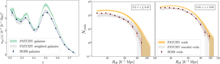
Figure 1. Left panel: number density of the BOSS DR12 and MultiDark PATCHY galaxies as a function of redshift. The BOSS data are represented with blue markers, and a spline fit is depicted by the dashed line. We report with a green band the galaxy number density of the 100 PATCHY mock realizations, distinguishing with different shades the 68% and 95% confidence levels. We represent the same distribution, but for mock galaxies weighted to mimic the BOSS survey completeness in gray. Central and right panels: number counts measured from the full sample of voids identified with VIDE, computed as a function of their effective radius and with a cut Reff > 30 h−1 Mpc. The two panels represent the void size function in the redshift ranges 0.2 < z ≤ 0.45 and 0.45 < z < 0.65, in red circles with error bars for the BOSS DR12 data and in orange bands for the MultiDark PATCHY mocks. The differently shaded bands show the 68% and 95% confidence levels around the mean value of the PATCHY void number counts. Gray bands represent PATCHY void counts after rescaling to the slightly smaller volume of the BOSS catalog.
Download figure:
Standard image High-resolution imageAs expected, the intrinsic higher mean density of the PATCHY galaxy catalog with respect to the BOSS one is reflected in the larger void numbers of these samples. The total number of voids identified with the void finder VIDE above a minimum effective radius of 30 h−1 Mpc is Nv = 3280 for the BOSS DR12 data and  as a mean value for the 100 PATCHY mock realizations. We note that in this estimate, as well as in the analysis we will present, we exclude galaxies with z > 0.65, since their number density is very low in this regime and extended objects like voids are potentially affected by the survey boundary.
We report in the rightmost panels of Figure 1 the size distribution of void number counts, dividing the sample in two bins of redshift, 0.2 < z ≤ 0.45 and 0.45 < z < 0.65, approximately coinciding with the two target selections LOWZ and CMASS. We show the void count size distribution from PATCHY via two shaded bands representing confidence levels of 68% and 95% as obtained from the 100 realizations. The corresponding uncertainty on the BOSS void number counts is computed by rescaling the PATCHY 68% errors by the square root of the ratio between BOSS and PATCHY survey volumes. Moreover, we use this survey volume ratio between PATCHY mocks and BOSS data to rescale the void counts in PATCHY, as shown in the two rightmost panels of Figure 1.
We computed the exact volume for these galaxy catalogs by summing up all Voronoi cells created by VIDE to tessellate the 3D space. This corresponds approximately to the total volume occupied by all of the voids identified by the algorithm. This approach also takes into account the removal of voids intersecting survey boundaries (see Sutter et al. 2015 for further details). The effective volumes derived with this procedure will be used in the following analysis also to convert the void number density predictions provided by the extended Vdn theory into void counts, Nvoids, to model accordingly the measured void size function.
As is evident from Figure 1, the size distribution of the rescaled PATCHY void counts matches the BOSS data closely. Only toward the small-scale cut, at Reff < 35 h−1 Mpc, do small deviations occur, which may be caused by finite resolution effects close to the mean galaxy separation  (see, e.g., Jennings et al. 2013; Pisani et al. 2015a; Ronconi & Marulli 2017; Contarini et al. 2019, 2022, for further details). Following our cleaning procedure, as described in Section 3.2, these small voids will be excluded in our analysis anyway. Finally, we note that the void counts from PATCHY can reach numbers below unity due to the averaging procedure over all mock catalogs.
3.2. Void Catalog Cleaning
The void sample provided by VIDE is not yet directly exploitable for the study of the void size function (Jennings et al. 2013; Ronconi & Marulli 2017), unless a number of ad hoc correction factors are introduced in order to link the cosmic voids found by the void finder with the ideal voids considered in the void size function theory. As introduced in Section 2, the Vdn model predicts the number counts of voids defined as spherical nonoverlapping regions embedding a specific density contrast value in the total matter field,  .
.
In this work, we adopt the complementary approach of aligning the considered sample of voids with the prescriptions of the Vdn model (as previously done by Contarini et al. 2019, 2021, 2022; Ronconi et al. 2019; Verza et al. 2019), therefore without modifying the void definition used in the theoretical model. To this end, we follow the cleaning methodology proposed by Jennings et al. (2013), applying an upgraded version of the code implemented by Ronconi & Marulli (2017). In this algorithm, the only settable parameter is the threshold  , which is computed in the density field of tracers (i.e., galaxies in this case) and is used to prepare the void sample. In this upgraded version of the cleaning algorithm, the galaxy density distribution is approximated as reported in the left panel of Figure 1, i.e., by a spline fit to the number density of galaxies as a function of redshift.
In our analysis, we follow the choice of Contarini et al. (2022) to select a threshold of  : this density contrast has been proven to represent a good compromise to model the innermost underdense regions of voids and simultaneously avoid poor statistics due to the sparsity of tracers. We underline that the selection of this threshold is not unique. We refer the reader to Contarini et al. (2022) for further details about the impact of this parameter choice.
Once the threshold  has been selected, the cleaning algorithm first discards from the original VIDE void catalog all of those underdensities having an internal spherical density contrast excessively high: starting from the void center identified by VIDE,
11
a sphere with starting radius Rcentral = 2 MGS(z) is grown, and if this sphere does not match the minimum requirement imposed by the chosen threshold, i.e.,
has been selected, the cleaning algorithm first discards from the original VIDE void catalog all of those underdensities having an internal spherical density contrast excessively high: starting from the void center identified by VIDE,
11
a sphere with starting radius Rcentral = 2 MGS(z) is grown, and if this sphere does not match the minimum requirement imposed by the chosen threshold, i.e.,  , the corresponding void is rejected. Second, all of the remaining underdensities are rescaled following the shape of their void density profile up to a radius R,
12
embedding a spherical density contrast equal to
, the corresponding void is rejected. Second, all of the remaining underdensities are rescaled following the shape of their void density profile up to a radius R,
12
embedding a spherical density contrast equal to  . Lastly, all of the mutually intersecting voids are removed by rejecting, one by one, the overlapping object with the higher central density.
The final outcome of this cleaning procedure is a sample of voids ideally free of spurious Poissonian fluctuations and shaped in agreement with the theoretical definition adopted in the void size function model. In particular, to match the void number counts measured from this sample and the void size function predicted by the extended Vdn model (see Section 2), we must convert the underdensity threshold used to rescale the voids,  in our case, by means of Equation (7); this allows us to recover the corresponding value in the total matter density field,
  , which then is inserted in Equation (2) after the transformation to its linear theory counterpart via Equation (4).
We show an example of the cleaned void samples obtained in this work in Figure 2, where we report 200 h−1 Mpc-thick slices of the BOSS DR12 and MultiDark PATCHY light-cones. In this visual representation, we depict galaxies and voids in the full redshift range 0.2 < z < 0.75, separating the observed BOSS data (top-left panels) from those corresponding to one of the 100 PATCHY mocks (bottom-right panels). As expected, we see a similarity between the projected distribution of galaxies and voids in the specular sky sections of the observed and simulated data. We also point out that any apparent overlapping between voids is given by projection effects within the slice and that the regions not featuring the presence of voids are those excluded by the survey mask.

Figure 2. Visual representation of the distribution of galaxies and voids in the BOSS DR12 data set and the MultiDark PATCHY simulations from a redshift range 0.2 < z < 0.75 and within a slice of width 200 h−1 Mpc. In the upper-left panels we show the northern and the southern galactic caps covered by BOSS, while in the lower-right panels the corresponding regions reproduced by one of the PATCHY mocks are shown. For each of the four represented sky areas, we indicate the cosmic voids identified in the distribution of galaxies by filled circles, post-processed with the cleaning procedure. For those voids that only partially intersect with the selected slice, we additionally show a dashed circle to indicate their full size that extends beyond the slice.
Download figure:
Standard image High-resolution image3.3. Cosmological Analysis
Now that the void size function theory and the void sample preparation have been outlined, we describe the Bayesian analysis we perform to investigate different cosmological scenarios and to calibrate the void size function model (see Section 3.4). According to Bayesian statistics, the posterior probability of a set of model parameters, Θ, given a data set,  , which is composed of the measured void number counts in our case, can be computed as
  , where
  is the likelihood, and p(Θ) is the prior distribution. Since in this work we consider the number counts of cosmic voids, the likelihood can be assumed to follow Poisson statistics (Sahlén et al. 2016):
where the product is over the radius and redshift bins, labeled with i and j, respectively. The quantity  is the number of voids in the ith radius bin and jth redshift bin, while N(ri
, zj
∣Θ) corresponds to the expected value in the considered cosmological model, given a set of parameters Θ.
is the number of voids in the ith radius bin and jth redshift bin, while N(ri
, zj
∣Θ) corresponds to the expected value in the considered cosmological model, given a set of parameters Θ.
The first cosmological scenario we investigate in this work is the standard flat ΛCDM model, characterized by six fundamental parameters: the total matter density parameter (Ωm), the dimensionless Hubble parameter (h ≡ H0/100 km s−1 Mpc−1), the baryon density parameter times h2 (Ωb h2), the spectral index of the primordial power spectrum (ns), the reionization optical depth (τ), and the primordial power spectrum amplitude (As), which we appropriately reinterpret with the present-time matter power spectrum normalization (σ8). In our modeling, we require flatness by imposing the cosmological constant-density parameter to be ΩΛ = 1 − Ωm and define the value of the cold dark matter component as Ωcdm = Ωm − Ωb. We underline that, analogously to σ8, the Universe density parameters defining the cosmological scenario are expressed with their present-day values.
In addition to the current standard model of cosmology, we also consider a Universe framework implementing a constant dark energy equation of state, which is commonly denoted wCDM. This model represents the simplest dark energy model alternative to ΛCDM, and is therefore characterized by an additional parameter, w. This scenario reduces to standard ΛCDM when w = −1.
In the Bayesian analysis reported in Section 4, both cosmological scenarios will be explored. We focus in particular on the cosmological degeneracies acting on the parameter planes Ωm–σ8, for the ΛCDM model, and Ωm–w, for the wCDM model. This selection is motivated by recent promising studies concerning the complementarity of different void statistics with standard cosmological probes, which showed the effectiveness of a joint analysis in constraining the growth of cosmic structures and the dark energy equation of state (Pisani et al. 2015a; Bayer et al. 2021; Bonici et al. 2022; Contarini et al. 2022; Hamaus et al. 2022; Kreisch et al. 2022; Pelliciari et al. 2023).
We sample the posterior distribution of the model parameters with a Markov Chain Monte Carlo (MCMC) technique, by considering wide uniform priors for the cosmological parameters of interest, i.e., Ωm and σ8 for the ΛCDM scenario, and Ωm and w for the alternative scenario. We marginalize over the remaining cosmological parameters (h, Ωb h2, ns, and τ for the first, and also σ8 for the second model) by assigning uniform priors centered on their corresponding values in the PATCHY simulation cosmology (Planck Collaboration et al. 2014) and with a total amplitude equal to 10× the 68% uncertainty provided by the Planck2018 results (Planck Collaboration et al.2020). We tested the effect of using different priors, considering the constraints given by the Planck2013 cosmology (Planck Collaboration et al. 2014), finding no or nonsignificant variations (<1.5%) on both the predicted cosmological values and their relative precision.
Two fundamental quantities to compute at each step of the MCMC procedure are the Hubble parameter, H(z), and the matter power spectrum, P(k). We calculate the former as

imposing w = −1 for the ΛCDM case, where Ωde = ΩΛ. The total matter power spectrum is instead evaluated with the approximations for the matter transfer function of Eisenstein & Hu (1999). All of the cosmological calculations (e.g., the 2PCF modeling reported in Appendix A), the Bayesian analyses, and the data catalog manipulations (including the void cleaning procedure described in Section 3.2) described in this work are performed in the numerical environment provided by the CosmoBolognaLib 13 (Marulli et al. 2016), a large set of free software C++/Python libraries composed of constantly growing and improving codes for cosmological analyses.
3.4. Model Calibration
As discussed in Section 2, to model the size function of cosmic voids identified in a biased tracer field, we need to estimate the effective bias of our mass tracers. For this purpose, we measure the redshift-space anisotropic 2PCF of the analyzed galaxies by means of the popular Landy & Szalay (1993) estimator. We then model the corresponding multipole moments with the theoretical prescriptions presented in Taruya et al. (2010), which take into account both the nonlinear gravitational clustering, redshift-space distortions, and galaxy bias. We refer the reader to Appendix A for a detailed description of the 2PCF modeling performed in this work.
We apply the galaxy clustering modeling procedure to the 100 PATCHY mock galaxy catalogs obtaining the correlation matrix of the 2PCF multipoles and the values of beff σ8 for each realization. By computing the median and the standard deviation of the 100 σ8-dependent bias values of the PATCHY galaxy mocks, we attain beff σ8 = 1.33 ± 0.02 and 1.26 ± 0.02, respectively for the two redshift bins considered in this analysis, i.e., 0.2 < z ≤ 0.45 and 0.45 < z < 0.65 (see Section 3.1). The corresponding values of the effective bias, achievable in this case knowing the true cosmology of the MultiDark PATCHY simulations, are beff = 1.94 ± 0.03 and 2.02 ± 0.03.
We use the values of beff
σ8 to calibrate the linear function  reported in Equation (7) by means of a Bayesian analysis of the number counts of PATCHY cleaned voids. To this end, we measure the median number counts of the 100 PATCHY samples of voids processed by the cleaning algorithm, fixing the minimum void radius at 2.5× the mean galaxy separation (MGS) computed at the mean redshift of the galaxies in the low- and high-redshift subsamples considered. This choice is in agreement with previous works (Contarini et al. 2019, 2021, 2022; Ronconi et al. 2019) and leads to the selection of voids with approximately Reff > 35 h−1 Mpc. A detailed discussion of the impact of this choice is presented in Appendix C.
Our goal is to fit both the median PATCHY void count data sets (i.e., featuring the two selected redshift ranges) to calibrate the free parameters, Cslope and Coffset, of the extended Vdn model described in Section 2.2. As for Bslope and Boffset, these coefficients are meant to take into account the galaxy bias variation with redshift, beff(z), so our parameterization is expected to hold in the full range of redshift covered by the survey. Nevertheless we notice that, if the galaxy samples extracted at different redshifts were characterized by incompatible intrinsic properties (e.g., different flux or mass limits), this relation is in fact expected to vary (Contarini et al. 2019), eventually deviating from linearity. In our case, the galaxy sample selection is restricted to two redshift bins only, so the linear relation calibrated encompasses any potential variation in the intrinsic properties of the sample.
We remind the reader that the calibrated values, as well as the relative covariance relation for these parameters, are expected to be different from those found in previous papers (i.e., Contarini et al. 2019, 2021, 2022) for Bslope and Boffset. In these works indeed,  was parameterized by means of beff only; therefore, the first coefficient of the linear function is positive, because of the increasing dependence of beff with redshift.
14
Conversely, the slope of the linear function
was parameterized by means of beff only; therefore, the first coefficient of the linear function is positive, because of the increasing dependence of beff with redshift.
14
Conversely, the slope of the linear function  is expected to be negative in our analysis given its dependence on beff
σ8, which is instead decreasing with redshift for the selected sample of galaxies.
is expected to be negative in our analysis given its dependence on beff
σ8, which is instead decreasing with redshift for the selected sample of galaxies.
We perform the Bayesian analysis starting by assuming the likelihood form expressed in Equation (9) and computing the covariance between our 100 PATCHY number count measures of the cleaned voids samples. We report the void counts covariance matrix, C
ij
, normalized by its diagonal component,  , in the left panel of Figure 3. We separate in this plot the low- and high-redshift ranges considered in our analysis, characterized by six and five logarithmic radius bins, respectively. We notice that the covariance between the void radii at the same redshift and between the two redshift bins exhibits negligible off-diagonal terms (as suggested by Kreisch et al. 2022). We tested the effect of modeling the void counts with a Gaussian likelihood including the full covariance matrix presented here, and we found no statistically relevant change in the results, confirming the low impact of the off-diagonal terms in this analysis. We finally note that the supersample covariance effects are expected to be small on the void size function, so its covariance can be reliably approximated without considering the presence of supersurvey modes (Bayer et al. 2022).

Figure 3. Left: covariance matrix (normalized by its diagonal components) of MultiDark PATCHY void counts, measured after the application of the cleaning procedure. The different radius bins (i, j) are divided by vertical and horizontal white lines to separate the two redshift intervals covered by the void number counts. Right: 68% and 95% 2D confidence contours obtained from the void size function model calibration. The maximum posterior values found for Cslope and Coffset are indicated with orange dotted lines and reported at the top of the upper and the right subpanels. The latter show the projected 1D posterior distribution of these parameters and the relative 68% uncertainty with a green shaded band.
Download figure:
Standard image High-resolution imageTo model the average void number counts extracted from the PATCHY mock catalogs and to calibrate the void size function nuisance parameters, we applied the extended Vdn model to the low- and high-redshift bins analyzed in this work. We consider the median redshifts of the two galaxy samples, assigning to each the corresponding value of the σ8-dependent bias as a Gaussian prior, with mean and standard deviation given by the 2PCF analysis. Then we set wide uniform priors for Cslope and Coffset, and sample the posterior distribution of these parameters, assuming the fiducial cosmology of the MultiDark PATCHY simulations.
We show the results of the nuisance parameter calibration in the right panel of Figure 3, where we report the 68% and 95% confidence contours on the parameters Cslope and Coffset. The values of the maximum posterior probability are reported at the top of the two panels representing the associated 1D posterior distribution projections. We notice that Cslope and Coffset are strongly anticorrelated, and that their posterior distribution is asymmetric. In particular, the skewness of the distribution is due to the physical requirement of  for the underdensity threshold, resulting from the Vdn model reparametrization.
In Figure 4 we report the calibrated Vdn model derived from the fitting procedure, together with the average void counts measured from the PATCHY mock catalogs. We show in the two panels of this figure the results for the low- and high-redshift bins analyzed, 0.2 < z ≤ 0.45 and 0.45 < z < 0.65. The markers indicate the number counts of cleaned voids, while the error bars are computed as the standard deviation of the 100 number count measures in each radius bin. We highlight that this uncertainty on the void counts is similar, although larger than the Poissonian error (i.e., the rms of the void counts), which represents an underestimation of the true error associated with the counts. The line indicates the theoretical prediction from the extended Vdn model, dependent on the value of beff σ8, characterizing the galaxies belonging to the considered redshift subsample. We report with a shaded band the 68% uncertainty on the void size function model, associated with the constraints on the parameters Cslope and Coffset, derived from the calibration on the MultiDark PATCHY simulations.

Figure 4. Median void counts as a function of their cleaned radius, measured from 100 mocks of the MultiDark PATCHY simulation and for the two redshift ranges considered this analysis: 0.2 < z ≤ 0.45 (left) and 0.45 < z < 0.65 (right). For each panel, we represent the median void number counts as orange diamonds, with error bars given by their standard deviation across the different PATCHY realizations. We indicate with a green line the calibrated void size function model, dependent on the value of beff σ8 of the redshift-selected sample of galaxies. The green shaded area represents the 68% confidence region around the calibrated model, determined by the confidence contour reported in the right panel of Figure 3.
Download figure:
Standard image High-resolution imageThe agreement between the measured void number counts and the theoretical predictions of the calibrated Vdn model proves the effectiveness of our methodology, which we exploit in this work following two different approaches. The first is to assume the exact values, i.e., without any associated uncertainty, for the parameters Cslope and Coffset obtained from the calibration of the model on the PATCHY mocks. This case corresponds to the ideal assumption of using volume-unlimited cosmological simulations perfectly reproducing the survey data that one wants to study or, alternatively, to have a size function model including a fully theoretical description of both the effects of redshift-space distortions and mass tracer bias. This approach has been explored from a theoretical point of view in recent works (e.g., Verza et al. 2022), but a complete and calibration-independent model has not yet been provided. Although optimistic, this first approach shows the full potential of the methodology and is useful to understand the limitations related to the calibration procedure; the analysis performed with fixed values of Cslope and Coffset will be labeled hereafter as fixed calibration.
The second approach consists of including the uncertainties derived from the calibration procedure: the entire posterior distribution of the parameters Cslope and Coffset, sampled using the PATCHY void number counts and reported in the right panel of Figure 3, is assumed as prior for the Bayesian analysis of the BOSS void size function. The analysis conducted with this methodology will be denoted as relaxed calibration, and provides more conservative cosmological constraints, due to the limits of the calibration procedure performed with the MultiDark PATCHY simulations. We refer the reader to Appendix C for further insights about the impact of the calibration parameter priors on the cosmological constraints from the void size function.
To validate the proposed modeling approaches, we derive mock cosmological constraints from the PATCHY void size function, with the aim of recovering the true cosmology of the simulation and evaluating the constraining power of the measured void number counts. We report the results of this test in Appendix B, where we prove the effectiveness of the model in retrieving the MultiDark PATCHY simulation input cosmological parameters within 68% errors, for both the assumed cosmological models (i.e., ΛCDM and wCDM). We also refer the interested reader to Appendix B for a discussion about the dependency of the void size function constraining power on the main characteristics of the analyzed data: the number density and volume coverage of the galaxy sample. As these two quantities differ between the PATCHY and BOSS catalogs, the precision of the cosmological constraints obtained from the corresponding void samples is also slightly different.
4. Results
4.1. BOSS DR12 Void Counts
Now that the void size function model has been calibrated, we are ready for the cosmological exploitation of the void number counts measured from the BOSS galaxy catalogs. To prepare the void sample, we follow the same pipeline applied to the PATCHY mocks. First, we clean the void catalogs extracted with VIDE, assuming the galaxy number density distribution reported in the left panel of Figure 1 and approximated with a spline function, which is represented as a dashed line. During the cleaning operation, we consider the same values for the density threshold,  , and for the void size selection, R > 30 h−1 Mpc. Then we extract from this sample the number of voids as a function of their radius for the two redshift ranges considered in this analysis (see Section 3.1). We finally compute the uncertainties on the binned void size function measures through a volume-based rescaling of the errors estimated for the PATCHY void number counts, as explained in Section 3.1 to describe the right panel of Figure 1.
These data sets, obtained with the fiducial Planck2013 cosmology (Planck Collaboration et al. 2014), need to be compared with the corresponding theoretical model of the void size function evaluated with the calibrated parameters Cslope and Coffset. To do this, we measure the value of the σ8-dependent bias, considering the BOSS galaxies belonging to the two selected redshift subsamples, and the 2PCF covariance matrix built by means of PATCHY mocks (see Sections 3.4 and Appendix B): we find beff σ8 = 1.36 ± 0.05 for the interval 0.2 < z ≤ 0.45 and beff σ8 = 1.28 ± 0.06 for 0.45 < z < 0.65. Thereafter, we use these values to compute the theoretical void size function by means of the extended Vdn model calibrated in Section 3.4, and we rely on the effective volume covered by the void finder applied to the BOSS galaxies to convert the predicted void number density into number counts, directly comparable with our observed data sets.
At this point we perform a Bayesian analysis of the measured void number counts by assuming the likelihood function reported in Equation (9) and testing the two cosmological models outlined in Section 3.3. For both the considered cosmological scenarios, i.e., ΛCDM and wCDM, we follow the two approaches presented in Section 3.4, which depend on the constraints assumed from the model calibration with PATCHY mock catalogs, i.e., the fixed calibration and the relaxed calibration methodologies.
In Figure 5 we show a comparison between the measured size function of voids identified in the distribution of BOSS DR12 galaxies and the best-fit model computed with the MCMC sampling technique. We report the results for the ΛCDM cosmological model, obtained treating the parameters Cslope and Coffset of the extended Vdn model as free, but restrained by a prior distribution determined from the PATCHY calibration constraints (i.e., the relaxed calibration case). We recall that in this specific analysis, the free cosmological parameters of the model are Ωm and σ8, while the remaining ones are bound to Planck2018 constraints (see Section 3.3 for a more detailed description). The MCMC technique used to sample the posterior distribution of all of these parameters provides us with the best-fit value and the corresponding uncertainty for the void size function model, represented in Figure 5 as a solid line surrounded by a shaded band covering the 68% confidence region.

Figure 5. Void counts as a function of their cleaned radius measured in the BOSS DR12 galaxy distribution, for the two redshift subsamples considered in this analysis: 0.2 < z ≤ 0.45 (left) and 0.45 < z < 0.65 (right). For each panel, we report with red circles the measured void size function, with error bars computed by rescaling those associated with the corresponding PATCHY void counts. We show in blue the void size function model calibrated with the PATCHY mock catalogs and dependent on the value of beff σ8 of the redshift-selected sample of galaxies. In this case, the best-fit model (solid line) and its 68% confidence region (shaded) are computed by fitting the measured void counts with a ΛCDM cosmology and leaving the parameters σ8 and Ωm free (see the relaxed calibration case of Section 3.4).
Download figure:
Standard image High-resolution imageWe point out the good agreement between the measured void number counts and the extended Vdn model in Figure 5, for both the low- (left panel) and high- (right panel) redshift ranges analyzed, featuring three and four independent radius bins, respectively. We highlight that the void number count binning applied here is the same as that used for the PATCHY analysis. In this case, however, the void counts are not derived from an averaging procedure over different realizations and therefore cannot be lower than unity. This fact, combined with the statistical rarity of large voids, leads to more restricted void size ranges with respect to those presented in Figure 4. Moreover, analogously to what we found for the PATCHY mocks, voids are more abundant in the high-redshift subsample, given the greater volume covered by the galaxies in the light-cone.
The data-model agreement obtained for the remaining modeling approach (i.e., the fixed calibration case) and for the alternative cosmological scenario considered (i.e., wCDM, assuming both types of calibration parameter priors) is similar to the results presented, which is why we do not explicitly show them here. Nevertheless, the cosmological constraints corresponding to each case will be described in the following section.
4.2. Cosmological Constraints
Figure 6 shows the constraints resulting from both void size function calibration approaches presented in this work. In the left panel we show the results for the ΛCDM scenario, while in the right we show those for the alternative wCDM model. We represent in different colors the 68% and 95% confidence contours for the two cases labeled fixed and relaxed calibration. We note that when relaxing the calibration constraints, the corresponding confidence contours slightly enlarge as a consequence of the contribution given by the variation of the parameters Cslope and Coffset. The main effect of the relaxed calibration approach is to loosen the constraining power on the parameters σ8 and w, for the ΛCDM and wCDM scenarios, respectively. On the other hand, as visible from the 1D marginalized posterior distributions reported in the subpanels of Figure 6, the corresponding impact on Ωm is statistically negligible.
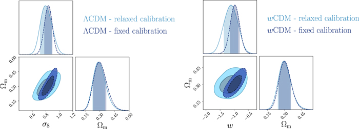
Figure 6. Constraints from the size function of voids identified in the BOSS DR12 data set, for ΛCDM (left) and wCDM (right) flat cosmologies. For both panels, the 2D contours indicate the 68% and 95% confidence levels on the posterior distribution of the main model parameters, while the 1D distributions show the marginalized posteriors of each parameter with the 68% confidence interval indicated as a shaded band. In dark blue we report the results obtained by fixing the parameters Cslope and Coffset to their maximum posterior values obtained from the model calibration with PATCHY mocks (fixed calibration). In light blue we show the constraints when assuming an uncertainty on Cslope and Coffset, given by their posterior distribution reported in the right panel of Figure 3 (relaxed calibration).
Download figure:
Standard image High-resolution imageOne of the most important features to notice is the orientation of the Ωm–σ8 confidence contour reported in the left panel of Figure 6. First, this degeneracy direction is in agreement with the results of other works that analyzed the void size function in simulated catalogs (Bayer et al. 2021; Kreisch et al. 2022). Second, as demonstrated by Contarini et al. (2022) and Pelliciari et al. (2023), it is orthogonal to that of other standard cosmological probes, such as galaxy clustering, weak lensing, and cluster number counts. The latter is a fundamental characteristic to be exploited in order to maximize the constraining power given by probe combinations, thanks also to the negligible correlation of the void size function with standard statistics of overdense objects. We provide some insights on the physical origin of the orthogonality of these constraints in Appendix D.
We report the maximum posterior values and the relative 68% errors derived from the BOSS void size function analysis in Table 1. As we discuss in more detail in S. Contarini et al. (2023, in preparation), the constraints we derived are compatible with the Planck2018 results (Planck Collaboration et al. 2020). Assuming the flat ΛCDM framework, we obtain a value of Ωm = 0.285 (Ωm = 0.293) for the relaxed (fixed) calibration approach, with a corresponding precision of about 21%. In the same model, we have σ8 = 0.793 (σ8 = 0.839) for the relaxed (fixed) calibration approach, with a precision of 10% (7%).
Table 1. Maximum Posterior Values and 68% Uncertainties Associated with the Confidence Contours Reported in Figure 6
| Model Calibration | ΛCDM | wCDM | ||||||
|---|---|---|---|---|---|---|---|---|
| Ωm | σ8 | Cslope | Coffset | Ωm | w | Cslope | Coffset | |
| Relaxed |

|

|

|

|

| −1.11 ± 0.24 |

|

|
| Fixed |

|

| −1.62 | 4.30 |

|

| −1.62 | 4.30 |
Notes. We present the results for the two cosmological scenarios analyzed in this work, i.e., ΛCDM and wCDM, in two separate sets of columns, grouping together the freely varied parameters of the corresponding model. The first row of the table presents the results obtained by modeling the size function of BOSS DR12 voids using the relaxed calibration method, while the second row reports the constraints when adopting the fixed calibration approach (see Section 3.4 for further details).
Download table as: ASCIITypeset image
As already mentioned, we expect a significant improvement of the precision on these parameters through the joint analysis of void counts with different cosmological probes. This is investigated in a companion paper (S. Contarini et al. 2023, in preparation), where we present a more specific and detailed analysis of the contribution given by cosmic void counts on two of the main current issues in cosmology: the tension between late and early probes on the Hubble constant H0,and the matter clustering strength parameterized by  (see, e.g., Di Valentino et al. 2021a,2021b, for a review).
For what concerns the flat wCDM scenario, we obtain Ωm = 0.293 (Ωm = 0.299), with a corresponding precision of 17% (16%) for the relaxed (fixed) calibration strategy. Then we compute w = −1.11 (w = − 0.97) for the relaxed (fixed) calibration approach, with a precision of 22% (16%). For both cases, the results are compatible with the constant w = −1, so in agreement with the benchmark ΛCDM model.
5. Conclusions
The goal of this paper was to provide the first cosmological constraints from the void size function. The void catalog has been extracted from the BOSS DR12 galaxies (Dawson et al. 2013), which still represents one of the best-suited spectroscopic catalogs for the purpose of void identification.
In this analysis we employ an extension of the popular Vdn model (Jennings et al. 2013), which takes into account the effect of the galaxy effective bias on the traced void density profile, as well as geometric and dynamic distortions on the observed void shape (see Section 2.2). This model includes two nuisance parameters, Cslope and Coffset, which describe the rescaling of the Vdn underdensity threshold by means of the galaxy bias coupled with the matter power spectrum normalization, i.e., the quantity beff σ8. In order to calibrate these nuisance parameters, we exploit the MultiDark PATCHY simulations, which are designed to reproduce the BOSS data clustering properties (Kitaura et al. 2016a).
We prepared the void catalogs by applying a cleaning procedure and conservative selection cuts (see Section 3.2) to ensure the void samples to be in agreement with the prescriptions of the void size function theory. We then used 100 PATCHY mocks to calibrate the parameters Cslope and Coffset and validate the statistical method. The latter was achieved by comparing the theoretical predictions of the extended Vdn model with the void average number counts measured in the MultiDark PATCHY simulation (see Sections 3.4 and Appendix B). We performed a Bayesian analysis of the BOSS DR12 void number counts assuming a Poissonian likelihood, and investigated two cosmological scenarios (see Section 3.3).
Considering a flat ΛCDM model, we constrained the present-day values of Ωm and σ8, obtaining Ωm = 0.29 ± 0.06 and  with the conservative relaxed calibration approach (see Section 3.4). On the other hand, in a flat wCDM model, we constrained the parameters Ωm and w, obtaining
  and w = −1.1 ± 0.2 following the most conservative approach. Our estimate of the parameter w is compatible with a value of −1 within the 68% confidence region of its posterior, so it reveals no statistical evidence against the standard ΛCDM model.
Despite the numerous tests performed in this work to validate the robustness of the methodology, further analyses might be required to fully evaluate all of the systematic uncertainties possibly associated with our results. Specifically, we emphasize the importance of investigating the potential influence of the halo population algorithm parameters on the resulting void catalog, as well as exploring the dependence of the model calibration parameters on the fiducial cosmology. Ultimately, these effects should be included in the void size function analysis, by marginalizing over the explored parameters. The full investigation of the possible sources of systematic errors is beyond the scope of this paper, and future works will be specifically dedicated to this task.
In conclusion, we stress the fact that the cosmological constraints derived with the void size function are very promising, especially in the perspective of a combination with other cosmological probes (Bayer et al. 2021; Kreisch et al. 2022). This is, in particular, due to the strong orthogonality on the Ωm–σ8 parameter plane between the confidence contours obtained with the void size function and overdensity-based probes, as demonstrated in Contarini et al. (2022) and Pelliciari et al. (2023).
We explore in detail the synergy with other cosmological probes in a companion paper (S. Contarini et al. 2023, in preparation), using the same void data set built from the BOSS DR12. Finally, we note that a considerable improvement in the precision of the cosmological constraints achieved in this work will be obtained by applying our methodology to the data of the upcoming wide-field surveys, like Euclid (Laureijs et al. 2011; Amendola et al. 2018), NGRST (Green et al. 2012), and LSST (LSST Dark Energy Science Collaboration 2012).
Acknowledgments
We sincerely thank the referee for providing insightful comments, which undoubtedly have led to the improvement of this work. S.C. thanks Michele Moresco, Alfonso Veropalumbo, Giorgio Lesci, and Nicola Borghi for the contribution and suggestions they provided. The authors thank Scott Dodelson, Steffen Hagstotz, Barbara Sartoris, Nico Schuster, and Giovanni Verza for useful conversations. We acknowledge the grant ASI n.2018-23-HH.0. S.C., F.M., L.M., and M.B. acknowledge the use of computational resources from the parallel computing cluster of the Open Physics Hub (https://site.unibo.it/openphysicshub/en) at the Physics and Astronomy Department in Bologna. A.P. is supported by NASA ROSES grant 12-EUCLID12-0004, and NASA grant 15-WFIRST15-0008 to the Nancy Grace Roman Space Telescope Science Investigation Team "cosmology with the High Latitude Survey." A.P. acknowledges support from the Simons Foundation to the Center for Computational Astrophysics at the Flatiron Institute. N.H. is supported by the Excellence Cluster ORIGINS, which is funded by the Deutsche Forschungsgemeinschaft (DFG, German Research Foundation) under Germany's Excellence Strategy—EXC-2094—390783311. L.M. acknowledges support from PRIN MIUR 2017 WSCC32 "Zooming into dark matter and proto-galaxies with massive lensing clusters." M.B. acknowledges support by the project "Combining Cosmic Microwave Background and Large Scale Structure data: an Integrated Approach for Addressing Fundamental Questions in Cosmology," funded by the MIUR Progetti di Ricerca di Rilevante Interesse Nazionale (PRIN) Bando 2017—grant 2017YJYZAH. We acknowledge use of the Python libraries NumPy (Harris et al. 2020), Matplotlib (Hunter 2007) and ChainConsumer (Hinton 2016).
Appendix A: Multipoles Modeling
In this appendix, we present the analysis of the galaxy two-point correlation function multipoles, performed on both the MultiDark PATCHY and BOSS DR12 data, to derive the linear effective bias. This quantity is fundamental to parameterize the void size function model we introduced in Section 2.2, and consequently to rescale the void radii according to the observed void density profile.
We measure the 2D redshift-space 2PCF with the Landy & Szalay (1993) estimator:

where μ is the cosine of the angle between the line of sight and the observed separation vector s ; GG(s, μ), RR(s, μ), and GR(s, μ) are the numbers of galaxy–galaxy, random–random, and galaxy–random pairs in bins of s and μ; NG and NR are the total numbers of galaxies and random objects; and NGG = NG(NG − 1)/2, NRR = NR(NR − 1)/2, and NGR = NG NR are the total numbers of galaxy–galaxy, random–random, and galaxy–random pairs, respectively. The 2PCF is measured on scales from 10–60 h−1 Mpc and in the two redshift ranges considered in this paper, i.e., 0.2 < z ≤ 0.45 and 0.45 < z < 0.65, assuming the fiducial cosmology of PATCHY simulations (see Section 3.1). For both real and mock galaxy samples, we make use of the random catalogs provided by the BOSS collaboration, which are built with the same geometry and redshift distribution of the target data set, but 50× denser.
We expand the 2D 2PCF into its multipole moments:

where ℓ is the degree of the Legendre polynomials Lℓ (μ). We consider the first three non-null multipole moments, i.e., the monopole, ξ0(s), the quadrupole ξ2(s), and the hexadecapole, ξ4(s):

where L0 = 1, L2 = (3μ2 − 1)/2, L4 = (35μ4 − 30μ2 + 3)/8.
We report the results of these measures in Figure A1, for both the 100 PATCHY mock realizations and BOSS catalogs. We notice the excellent agreement between the clustering properties of mocks and real data in each of the redshift ranges considered. Minor mismatches are found for the hexadecapole moment, although these deviations are significant only at small spatial scales, which are not considered in the following modeling of the analysis.
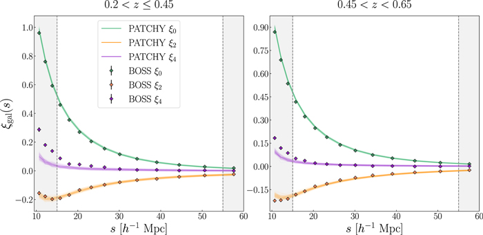
Figure A1. MultiDark PATCHY and BOSS DR12 measurements of the redshift-space galaxy 2PCF multipoles, in the two redshift ranges considered in this analysis: 0.2 < z ≤ 0.45 (left) and 0.45 < z < 0.65 (right). Solid lines show the data obtained from the 100 PATCHY mock catalogs, while round markers indicate the measures from the BOSS data set. The correlation function monopole (ξ0), quadrupole (ξ2), and hexadecapole (ξ4) are represented in green, orange, and violet, respectively. The shaded regions outside the range 15 < s [h−1 Mpc] < 55 are those excluded from the statistical analysis.
Download figure:
Standard image High-resolution imageWe use the 100 measures of the two-point correlation multipoles performed on the PATCHY mocks to estimate the covariance matrix as

where y = (ξ0, ξ2, ξ4) is the combined vector of monopole, quadrupole, and hexadecapole,  is the mean value computed by averaging the measures from the different realizations, k runs over the different mock realizations, Ns
= 100, and (i, j) define the galaxy separation bins. We show the results for the two redshift subsamples considered in Figure A2. The correlation is found to be statistically relevant between the different separation bins, though almost negligible between the three 2PCF multipoles.
is the mean value computed by averaging the measures from the different realizations, k runs over the different mock realizations, Ns
= 100, and (i, j) define the galaxy separation bins. We show the results for the two redshift subsamples considered in Figure A2. The correlation is found to be statistically relevant between the different separation bins, though almost negligible between the three 2PCF multipoles.

Figure A2. Covariance matrix (normalized by its diagonal components) of the MultiDark PATCHY redshift-space galaxy 2PCF multipoles, for the two redshift selections considered in this analysis: 0.2 < z ≤ 0.45 (left) and 0.45 < z < 0.65 (right). The galaxy separation bins (i, j) are divided by vertical and horizontal white lines to separate the measures of the monopole (ξ0), quadrupole (ξ2), and hexadecapole (ξ4) moments of the correlation function.
Download figure:
Standard image High-resolution imageWe adopt this covariance matrix in the Bayesian analysis to model the 2PCF multipoles in order to constrain the galaxy effective bias. We assume a standard Gaussian likelihood defined as follows:

where N is the number of separation bins at which the multipole moments are computed, C −1 is the precision matrix, i.e., the inverse of the covariance matrix, and superscripts refer to data (d) and model (m).
To model the multipoles of the redshift-space 2PCF, we apply the approximation introduced by Taruya et al. (2010), which has been extensively tested and validated in the literature (see, e.g., de la Torre & Guzzo 2012; Pezzotta et al. 2017; García-Farieta et al. 2020). According to this model, the redshift-space dark matter power spectrum can be expressed as follows:
where f is the linear growth rate, b is the linear bias, σv is the pairwise velocity dispersion, and D is a damping factor that characterizes the random peculiar motions at small scales, assumed in this case to be Gaussian, i.e., ![$D(k,f,\mu ,{\sigma }_{{\rm{v}}})=\exp [-{k}^{2}{f}^{2}{\mu }^{2}{\sigma }_{{\rm{v}}}^{2}]$](https://content.cld.iop.org/journals/0004-637X/953/1/46/revision1/apjacde54ieqn54.gif) (Davis & Peebles 1983; Fisher et al. 1994; Zurek et al. 1994). Then Pδ
δ
(k) is the real-space matter power spectrum, and Pδ
θ
(k) and Pθ
θ
(k) are the real-space density-velocity divergence cross-spectrum and the real-space velocity divergence auto-spectrum, respectively. Lastly, in Equation (A6), cA and cB represent two additional terms to correct for systematic effects at small scales, which are computed according to Taruya et al. (2010) and de la Torre & Guzzo (2012), and can be expressed as a power series expansion of b, f, and μ (see Appendix A of Taruya et al. 2010, for details about the calculation of these correlation terms).
(Davis & Peebles 1983; Fisher et al. 1994; Zurek et al. 1994). Then Pδ
δ
(k) is the real-space matter power spectrum, and Pδ
θ
(k) and Pθ
θ
(k) are the real-space density-velocity divergence cross-spectrum and the real-space velocity divergence auto-spectrum, respectively. Lastly, in Equation (A6), cA and cB represent two additional terms to correct for systematic effects at small scales, which are computed according to Taruya et al. (2010) and de la Torre & Guzzo (2012), and can be expressed as a power series expansion of b, f, and μ (see Appendix A of Taruya et al. 2010, for details about the calculation of these correlation terms).
We estimate the power spectra Pδ δ (k), Pδ θ (k), and Pθ θ (k) in the standard perturbation theory, i.e., by expanding these statistics as sums of infinite terms, each one corresponding to an n-loop correction (see, e.g., Gil-Marín et al. 2012). Following García-Farieta et al. (2020) and Marulli et al. (2021), we consider in our analysis the corrections up to the one-loop order, computing the terms of the one-loop contribution with the CPT Library 15 (see also Bernardeau et al. 2002; Gil-Marín et al. 2012).
The power spectrum multipoles are finally calculated from Equation (A6) as

which is translated into configuration space by means of the following equation:

where jℓ are the spherical Bessel functions of order ℓ. We model the clustering multipole moments at scales 15 < s [h−1 Mpc] < 55, estimating the linear bias of the galaxy samples considered in this work.
We assign wide positive priors to the free parameters of the Taruya et al. (2010) model, i.e., b(z) σ8(z), f(z) σ8(z), and σv, maximizing their posterior distributions through a Bayesian analysis, on the 100 PATCHY mock galaxy catalogs. We compute the average and the standard deviation of the best-fit values obtained with PATCHY mocks to estimate beff σ8 and its uncertainty, respectively, for both the selected redshift subsamples. We apply the same modeling procedure to the BOSS DR12 galaxies, performing in this case an MCMC analysis to sample the full posterior distribution of the free model parameters, marginalizing over f(z) σ8(z) and σv, obtaining the values of beff σ8 reported in Section 3.4.
Appendix B: Method Validation
Here, we validate our data analysis method on the MultiDark PATCHY simulations using the void size function model calibrated in Section 3.4. This exercise is meant to check the validity of the methodology we introduced in this work and to quantify the impact of the survey characteristics on the resulting cosmological constraints from void counts.
We apply the Bayesian analysis described in Section 3.3 on the average void number counts reported in Figure 4, considering both the fixed and relaxed calibration approaches. Figure B1 shows the results for the two cosmological models tested in this work, i.e., the flat ΛCDM and wCDM model. In both scenarios we recover the true cosmological parameters of the simulation within 68% of uncertainties, confirming the reliability of the adopted pipeline.

Figure B1. Same as in Figure 6, but for the test constraints obtained from the size function of voids identified in the 100 mock catalogs of the MultiDark PATCHY simulations. Dark and light green colors indicate the results obtained by fixing and relaxing the calibration of the parameters Cslope and Coffset, respectively. The white star shows the input cosmological parameters of the simulation.
Download figure:
Standard image High-resolution imageAs expected, the orientation and shape of the confidence contours are analogous to those presented in Figure 6 for the BOSS galaxies. The results we present in Table B1 are compatible with those reported in Table 1, although with smaller uncertainties. By comparing these results, we notice that the main difference is in the precision on Ωm, which improves by a factor ∼1.7. However, this is not only due to the change of the volume coverage between BOSS and PATCHY galaxy catalogs. By comparing the square root of the effective volumes explored by VIDE (see Section 3.1), we find that the two samples merely differ by a factor of ∼1.33. We also have to consider the higher galaxy number density and the more extended void radius range covered by the PATCHY samples with respect to the BOSS data set (see Figure 1). These specifics play a role in further improving the constraining power of the void size function, by increasing the statistical relevance of the void catalog and extending the spatial scales on which the Vdn model is sampled. This result highlights the importance of taking into account the impact of both the volume coverage and the tracer number density on void numbers for the design of future redshift surveys.
Table B1. Maximum Posterior Values and 68% Uncertainties Associated with the Confidence Contours Reported in Figure B1
| Model Calibration | ΛCDM | wCDM | ||||||
|---|---|---|---|---|---|---|---|---|
| Ωm | σ8 | Cslope | Coffset | Ωm | w | Cslope | Coffset | |
| Relaxed |

|

|

|

|

|

|

|

|
| Fixed |

|

| −1.62 | 4.30 |

| −1.00 ± 0.11 | −1.62 | 4.30 |
Note. The description is analogous to that in Table 1, but for the test constraints obtained from the MultiDark PATCHY mocks.
Download table as: ASCIITypeset image
Despite the different characteristics of the PATCHY catalogs leading to an overall increase in the precision on the cosmological parameters with respect to the BOSS data, we note that part of the constraining power is absorbed by the Vdn model nuisance parameters Cslope and Coffset, when not kept fixed to their best-fit values. This shows how a rigorous calibration of these parameters is fundamental to maximize the effectiveness of the void size function as a cosmological probe (Contarini et al. 2021; Verza et al. 2022).
Appendix C: Systematic Errors
In this appendix, we evaluate the impact of the main systematic uncertainties possibly affecting our cosmological constraints by repeating the analysis on the PATCHY void counts considering different assumptions. We will focus on the relaxed calibration approach only, as it provides the most reliable constraints.
C.1. Calibration Uncertainties
We perform here the analysis on the PATCHY mocks by increasing the statistical errors of the void number counts. Specifically, during the calibration procedure, we associate to void counts Poissonian errors multiplied by factors of 2, 3, and 4. This approach is aimed at reproducing the effect of calibrating the void size function using mock catalogs with volumes 4×, 9×, and 16× smaller, respectively.
In the upper panel of Figure C1 we show the 2D posterior distribution of the parameters Cslope and Coffset, for the three analyzed cases. We note that the enlargement of the confidence contours is mainly restricted to the degeneracy direction of the two calibration parameters. In the lower panels of Figure C1 we show instead the test constraints obtained for the parameter planes Ωm–σ8 (ΛCDM scenario) and Ωm–w (wCDM scenario). In all of the presented cases, the true values of the simulation cosmological parameters remain in the 68% confidence region of the posterior distributions. As expected from the comparison between the relaxed calibration and fixed calibration methods (see Figure B1), the impact of the nuisance parameter prior on Ωm is almost negligible, especially in the ΛCDM case. In fact, the relative error on Ωm is stable around 14%. The effect on the constraints on σ8 and w is instead more important because of their degeneracy with the calibration parameters. The relative error on σ8 increases from 9%–23%, when increasing the calibration errors from 2–4× the Poissonian error. Analogously, the relative error on w increases from 18%–25%. However, we underline that the effects shown in this test are derived from extreme calibration scenarios.
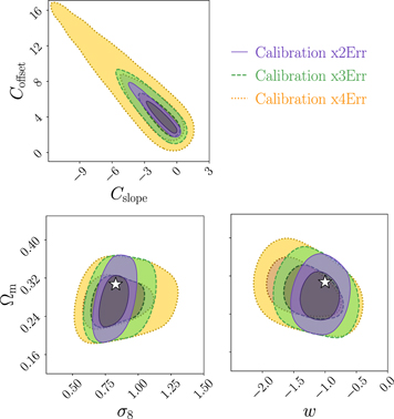
Figure C1. Shown here are 68% and 95% confidence contours obtained from the modeling of PATCHY void counts. Top: confidence contours in the Cslope–Coffset parameter plane, computed by increasing the void count uncertainty by factors of 2, 3, and 4. Bottom: confidence contours in the parameter planes Ωm–σ8 (right) and Ωm–w (left). These contours are derived using the distributions shown in the top panel as 2D priors for the calibration parameters. The white star indicates the true cosmological values of the PATCHY simulations.
Download figure:
Standard image High-resolution imageC.2. Fiducial Cosmology
In this section we repeat the whole analysis, assuming a fiducial cosmology that is different from that of Planck2013. We run the void finder and the cleaning procedure on the 100 PATCHY catalogs, considering a value of Ωm either decreased or increased by 3× the standard deviation reported in Planck Collaboration et al. (2020). Specifically, for this test we assume Ωm = 0.279 (−3σ) and Ωm = 0.335 (+3σ), modifying the value of Ωde to maintain Universe flatness. Moreover, we highlight that the accepted void radius range is recomputed during the analysis according to the value of MGS(z) in the considered cosmology.
We show in Figure C2 the 2D posterior distributions obtained for the parameter spaces Ωm–σ8 and Ωm–w. The two confidence contours are statistically compatible with each other, and the true cosmological values of the PATCHY simulations are recovered within the 68% uncertainty in both cases.
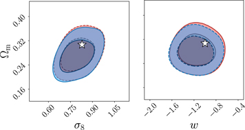
Figure C2. Shown here are 68% and 95% confidence contours computed by assuming different fiducial cosmologies in the modeling of PATCHY void counts, for the ΛCDM cosmology (Ωm–σ8 plane, right) and the wCDM (Ωm–w plane, left). In blue and red, we report the results derived for a flat cosmological model with Ωm = 0.279 and Ωm = 0.335, respectively. The white star indicates the true cosmological parameters of the PATCHY simulations.
Download figure:
Standard image High-resolution imageWe report in Table C1 the corresponding marginalized constraints computed, for the ΛCDM and wCDM scenarios. We note that, especially when exploring fiducial Ωm values lower than the true one (see the Ωm = 0.279 case), the underestimation of these cosmological parameters starts to become statistically significant. This issue will be analyzed in detail in future works.
Table C1. Maximum Posterior Values and 68% Uncertainties of the Cosmological Constraints Computed Assuming Ωm = 0.279 and Ωm = 0.335 as Fiducial
| ΛCDM | Ωm | σ8 |
|---|---|---|
| Fiducial Ωm = 0.279 |

|

|
| Fiducial Ωm = 0.335 |

|

|
| wCDM | Ωm | w |
| Fiducial Ωm = 0.279 |

|

|
| Fiducial Ωm = 0.335 |

|

|
Note. We report the results for both the ΛCDM (upper rows) and wCDM (lower rows) scenarios. The associated confidence contours are shown in Figure C2.
Download table as: ASCIITypeset image
C.3. Void Radius Selection
As a final test on systematic errors, we focus here on the void radius selection. The choice regarding the minimum acceptable void radius holds significant importance, as it directly impacts the strength of the resulting constraints: the greater the number of small voids included in the analysis, the more stringent the constraints derived from the void number counts. However, it is equally crucial to exclude the spatial scales that are influenced by void count incompleteness. In fact, the resolution of the tracer catalog affects the identification of small voids, which may be lost because of the Poisson noise.
In this work, we restricted our cleaned void sample to radii larger than 2.5× the MGS of the galaxy catalog (see Sections 3.1 and 3.4). This leads to a minimum void radius of about  and 35.13 h−1 Mpc, for the redshift bins 0.2 < z ≤ 0.45 and 0.45 < z < 0.65, respectively. For simplicity, we apply the same radius cut to both redshift bins, without relying on the MGS value. Here, we consider three different radii selections: one slightly lower than that used in the main analysis of this work, i.e.,
  , and two higher, i.e.,
  and 40 h−1 Mpc.
In Figure C3 we show the 2D posterior distributions computed for the ΛCDM and the wCDM scenarios by applying the presented radius selections. As expected, the cosmological constraints become weaker as the void minimum radius becomes larger. In the ΛCDM scenario, moving from the lowest to the highest radius cut, the relative error increases by factors of 1.9 and 1.2, for Ωm and σ8, respectively. When considering the wCDM scenario, the increase is instead by a factor 1.6, for both the parameters Ωm and w. However, it is important to emphasize that, in all three cases, the true cosmological parameters of the PATCHY simulations are within the 68% confidence region.
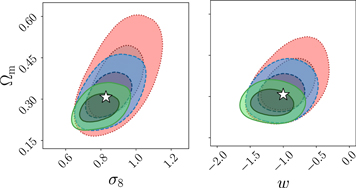
Figure C3. Same as in Figure C2, but for different void radius selections. We represent in green, blue, and red the test constraints derived by modeling the PATCHY void counts with  , respectively. The first radius selection is slightly lower than that used in the analysis presented in Appendix B.
Download figure:
Standard image High-resolution imageAppendix D: Parameter Orthogonality
The orthogonality on the Ωm–σ8 parameter plane between the void size function and the standard probes can be understood based on the following observations. Let us first consider the effects of these cosmological parameters on the linear matter power spectrum. Its variance determines both the number density of voids and galaxy clusters, or similarly dark matter halos (see Section 2).
Increasing the value of σ8 is equivalent to shifting the normalization of the power spectrum at z = 0 toward higher values, favoring the growth of matter perturbations. This enhances the formation of both galaxy clusters and cosmic voids. On the other hand, suppose we fix the matter power spectrum normalization σ8, and increase the matter density of the Universe, Ωm. As shown in the left panel of Figure D1, widely extended objects such as voids (10 ≲ r [h−1 Mpc] ≲ 100) correspond to cosmic scales characterized by a negative power spectrum response to an increase in Ωm. On the contrary, smaller cosmological objects, such as galaxy clusters (0.5 ≲ r [h−1 Mpc] ≲ 5) are characterized by a positive response. The spatial scale that separates the two matter power spectrum trends in this plot corresponds to k = 0.4 h Mpc−1, but depends on multiple factors, e.g., the redshift and the cosmological model. Moreover, during their nonlinear evolution, clusters decrease and voids increase their comoving sizes by up to a factor of a few. However, this is not enough to revoke the difference in their Lagrangian scales when selected in Eulerian space.
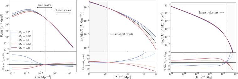
Figure D1. Theoretical linear matter power spectrum (left), void size function (center), and halo mass function (right) at z = 0.5, computed with Planck2013 parameters (Planck Collaboration et al. 2014), and normalized to have σ8 = 0.83. We represent in different colors the results of varying Ωm and highlight with a dotted vertical line the pivot points that separate opposite trends. The bottom subplots show the residuals from the fiducial model with Ωm = 0.3.
Download figure:
Standard image High-resolution imageIntuitively, for a given value of σ8, so when the clustering strength is fixed, the formation of voids is disfavored with increasing Ωm. This is because it makes large voids less underdense, while the collapse and accretion rate of overdensities is enhanced by the presence of more matter in the Universe. The counteractive behavior of these objects determines the complementarity of the constraints derived from the cluster mass function and the void size function (see also Pelliciari et al. 2023).
We substantiate this intuition in the center and right panels of Figure D1, where we illustrate the effects of variations in Ωm on the void size function (Jennings et al. 2013) and the halo mass function (Press & Schechter 1974). It is evident how the trends of the two statistics are opposite in the typical radius and mass ranges: higher values of Ωm cause a decrease in the number of cosmic voids and an increase in the number of massive halos. Nevertheless, this behavior is different for very small voids and the most massive halos. In this example, the pivot points correspond to R = 21 h−1 Mpc for voids and M = 1.7 × 10¹⁵ h−1 M⊙ for halos. We note, however, that very small voids (R ≃ 10 h−1 Mpc) are commonly not identified in wide-field surveys, because of their limited spatial resolution given by the tracer density. On the other hand, very massive clusters (M ≃ 1015 h−1 M⊙) are statistically very rare and constitute a minor contribution to the mass function constraints.
We finally underline that the reported statistics are just meant to portray a simplified view on the subject, and do not aim at reproducing any realistic distribution of cosmological objects. Indeed, a number of observational effects 16 modify the theoretical predictions of these models, leading to a shift of the pivot scales.
Footnotes
- 8
All of the quantities computed in linear theory are indicated in this work by the superscript "L." We will also mark the nonlinear ones with the superscript "NL" when it is necessary to distinguish.
- 9
 is the linear density contrast associated with the formation of voids, while with the collapse of dark matter halos. The value of the former is in an Einstein–de Sitter scenario; this value, however, cannot be directly used to model voids identified in a realistic tracer field (Contarini et al. 2019) and should be properly corrected to match the properties of the selected void sample (see details in Section 3.2). The latter can generally vary in the range , given by the turn-around and the collapse linear thresholds in an Einstein–de Sitter model. Nevertheless, we note that the variation of the quantity affects only the number of very small voids, which are not included in our analysis.
 - 10
- 11
We note that relying on the VIDE void center includes, to some extent, knowledge about the void shape, since it is computed as barycenter of all of the tracers composing the density depression (see Section 3.1).
- 12
We highlight the different notation with respect to the effective radius of voids not processed by the cleaning procedure, i.e., Reff.
- 13
- 14
This is true except for galaxy samples characterized by strong survey selection effects.
- 15
- 16
For instance, the mass tracer bias and the AP correction affect the void size function, and the inclusion of the baryon component inside dark matter halos affects the halo mass function.


