


Abstract
We present the observational results of a precursor of glycine, methylamine (CH3NH2), together with methanol (CH3OH) and methanimine (CH2NH) for the high-mass star-forming regions NGC 6334I, G10.47+0.03, G31.41+0.3, and W51 e1/e2 using the Atacama Large Millimeter/submillimeter Array. The molecular abundances of these sources were derived using the CASSIS spectrum analyzer and compared with our state-of-the-art three-phase chemical model NAUTILUS. We found that the observed abundance ratio of CH3NH2/CH3OH is between 0.008 and 1.0 for all sources, except for NGC 6334I MM3, where a ratio less than 0.002 is found. This may be due to its later evolutionary stage relative to the other cores. We also found that the observed CH3NH2/CH3OH ratio agrees well with the three-phase chemical model NAUTILUS, which includes the formation of CH3NH2 on the grain surface via a series of hydrogenation processes of HCN. This result clearly shows the importance of hydrogenation processes to form CH3NH2.
Export citation and abstract BibTeX RIS

Original content from this work may be used under the terms of the Creative Commons Attribution 4.0 licence. Any further distribution of this work must maintain attribution to the author(s) and the title of the work, journal citation and DOI.
1. Introduction
It has been proposed that the first steps in the chemical evolution toward the origin of life could have taken place in molecular clouds and continued within protoplanetary disks, followed by their delivery to the early Earth by comets and asteroids (Ehrenfreund et al. 2002). However, the synthesis and evolution of organic molecules, which form the building blocks of more complex biotic molecules, are not well understood. Over the last several years, there have been significant advances in this field thanks to dedicated searches for molecules of biological importance in the interstellar medium (ISM) and the atmospheres of comets. Among them, observations in the direction of the Galactic center toward Sgr B2(N) with the Green Bank Telescope (GBT) have led to the detection of interstellar aldehydes, namely propenal (CH2CHCHO) and propanal (CH3CH2CHO; Hollis et al. 2004) and simple aldehyde sugars like glycolaldehyde (CH2OHCHO; Hollis et al. 2000) in the ISM. Recently, McGuire et al. (2016) detected propylene oxide (CH3CHCH2O) for the same source. This is the first molecule detected in interstellar space that has the property of chirality, making it a leap forward in our understanding of how prebiotic molecules are made in the universe. In the era of the Atacama Large Millimeter/submillimeter Array (ALMA), the detection of the branched alkyl molecule isopropyl cyanide (i-C3H7CN) in Sgr B2(N) also gave us clues to the presence of amino acids in the ISM due to its critical side-chain structure (Belloche et al. 2014). Amino acids are the building blocks of life, and this is why the search for amino acids and their complex organic precursors at different stages of star and planet formation is one of the exciting topics in modern astronomy. Since glycine is the simplest amino acid and the only nonchiral member out of the 20 standard amino acids, it has received attention from a large number of researchers. Recently, volatile glycine (NH2CH2COOH) was detected in the coma of comet 67P/Churyumov-Gerasimenko by the Rosetta Orbiter Spectrometer for Ion and Neutral Analysis (ROSINA) mass spectrometer (Altwegg et al. 2016), supporting glycine's interstellar origin. In addition, the Hayabusa2 mission returned material to Earth from the asteroid Ryugu, giving us the opportunity to investigate the chemistry of a pristine extraterrestrial body. As a result, at least 23 amino acids in Ryugu aliquot are reported (Nakamura et al. 2022).
Revealing the formation pathways to glycine is an important topic for astrochemistry and astrobiology. Though there was a huge progress in our knowledge about how complex organic molecules (COMs) are built in the ISM, our knowledge of amino acids and their precursors is still limited. High-mass star-forming regions are the ideal sources to study the chemical evolution of COMs thanks to their high gas density and warm environment that enhance molecular evolution through the thermal hopping of molecules on grains (e.g., van der Tak 2005). In this context, formation processes to glycine in high-mass star-forming regions have been studied by many authors. Blagojevic et al. (2003) suggested that protonated hydroxylamine (NH2OH+) can react with acetic acid (CH3COOH) in the gas phase to form glycine. The importance of grain surface chemistry is emphasized as well. CH3NH2 can react with CO2 to form glycine under the radiation of UV photons or cosmic rays (Holtom et al. 2005; Lee et al. 2009). Singh et al. (2013) suggested that glycine can be formed via successive gas-phase radical–radical and radical–molecule reactions of simple species, such as CH2, NH2, CH, and CO. Of the precursors of glycine, recent works have improved our understanding of CH3NH2 chemistry. Experimentally, Kim & Kaiser (2011) reported the formation of CH3NH2 after electron and photon irradiation on interstellar ice analogs consisting of CH4 and NH3. This path would involve the recombination of radical species, CH3 and NH2 (CH3 + NH2 → CH3NH2), which are the products of decomposition of CH4 and NH3. Another candidate pathway could be successive hydrogenation processes of HCN (HCN + 2H → CH2NH, and CH2NH + 2H → CH3NH2; Woon 2002; de Jesus et al. 2021). Theule et al. (2011) experimentally demonstrated this formation process using interstellar ice analogs containing HCN. The inverse hydrogen subtraction process, CH3NH2 + H → CH2NH2, is also experimentally observed in Joshi & Lee (2022) at 3.2 K, suggesting that their abundances are in a quasi-equilibrium state.
Chemical kinetic models, where the evolution of molecular abundances are numerically solved with thousands of reactions along with the physical evolution of the star, are essential tools to test the importance of formation paths. The formation processes of glycine's precursors have been discussed in chemical model studies. Garrod (2013) has compared several possible processes to form glycine, including both gas-phase and grain surface reactions and suggested that with a model for a high-mass star-forming region (fast warm-up model), glycine is most efficiently formed via the reaction between CH2NH2 and COOH radicals, where the COOH radical is formed from the destruction of HCOOH. Suzuki et al. (2018) extended this work and suggested the acceleration of glycine formation by the photochemical reactions of CH3NH2 and CO2, which was supported by experiments (Lee et al. 2009). In either case, CH3NH2 may play an important role in the formation of glycine. The detections of CH3NH2 in the Murchison meteorite suggest that the formation of CH3NH2 can take place under extraterrestrial conditions (Pizzarello et al. 1994; Altwegg et al. 2016). Altwegg et al. (2016) also detected glycine and CH3NH2 in the coma of comet 67P/Churyumov-Gerasimenko, pointing out a chemical link between them considering their coexistence. With a chemical model, Suzuki et al. (2016) showed that CH3NH2 is formed on grains via successive hydrogenation processes of HCN and CH2NH, which agrees with previous studies (Theule et al. 2011). On the other hand, Suzuki et al. (2016) unexpectedly reported that the grain surface production of CH2NH is less important to explain the gas-phase CH2NH due to its rapid conversion to CH3NH2 on grains. Instead, CH2NH is efficiently formed via the gas-phase reaction CH3 + NH → CH2NH + H. Such proposed theoretical formation processes must be confirmed by observations of actual star-forming regions. The number of studies of glycine precursors in low-mass star-forming regions is small. CH2NH was detected in a solar-Like protostar, IRAS16293-2422B, as a part of the ALMA-PILS project (Ligterink et al. 2018), and in the molecular cloud L183 and the translucent cloud CB17 (Turner et al. 1999).
On the other hand, the detection of potential glycine precursors in high-mass star-forming regions has been reported by many authors. So far, many authors claimed the detection of CH3NH2. In the Sgr B2 region, the detection of CH3NH2 was reported almost 50 yr ago (Fourikis et al. 1974; Kaifu et al. 1974). More recently, Belloche et al. (2013) presented the detection of CH3NH2 in Sgr B2 (N) and (M) with the IRAM 30 m telescope. G10.47+0.03 is another interesting high-mass star-forming region where CH3NH2 and CH2NH is reported. Though the survey of other high-mass star-forming regions by Ligterink et al. (2015) could not confirm CH3NH2, Ohishi et al. (2019) succeeded in the detection of CH3NH2 in G10.47+0.03 with the NRO 45 m telescope. Since the excitation temperature of CH3NH2 is less than 46 K, the observed CH3NH2 would be in a cold envelope surrounding the hot core, suggesting the formation of this species through low-temperature chemistry, such as a hydrogenation process on grains. In NGC 6334I, Bøgelund et al. (2019) confirmed the detection of CH3NH2 in three clumps called MM1, MM2, and MM3. Furthermore, tentative detection of CH3NH2 was reported in the Orion Hot core (Pagani et al. 2017). The distribution of CH2NH is also widely known. CH2NH is detected in Sgr B2(OH), (N), (M), and (NW; Godfrey et al. 1973; Turner 1989; Sutton et al. 1991; Nummelin et al. 1998; Halfen et al. 2013). Halfen et al. (2013) showed that CH2NH and CH3NH2 in Sgr B2 (N) have different excitation temperatures, 44 ± 13 and 159 ± 30 K, respectively, suggesting that they exist in different environments. Jones et al. (2008, 2011) found the distribution of CH2NH from Sgr B2(N) to (S) at 3 mm and 7 mm with the MOPRA telescope. Many authors reported CH2NH in other high-mass star-forming regions, W51 e1/e2, Orion KL, G34.3+0.15, G19.61-0.23, G10.47+0.03, G31.41+0.3, NGC 6334I, and DR21(OH) (Dickens et al. 1997; White et al. 2003; Qin et al. 2010; Suzuki et al. 2016). Widicus Weaver et al. (2017) added a new detection of CH2NH in GCM+0.693-0.027, the shocked region located in the Sgr B2 complex, the massive hot core G12.91-0.26, and G24.33+00.11 MM1. Since glycine's precursors are well known in high-mass star-forming regions, it is possible to investigate their formation paths by comparing observational results and chemical models.
CH3OH is one of the most abundant COMs in star-forming regions, and it is known to be formed via the hydrogenation of CO (CO + 2H → H2CO and H2CO + 2H → CH3OH), which is very similar to the predicted formation path of CH3NH2 (HCN + 2H → CH2NH and CH2NH + 2H → CH3NH2). Therefore a comparison of the column densities of CH3NH2 and CH3OH may be useful to characterize the formation process of CH3NH2.
In this paper, we report ALMA observations of CH3NH2, CH2NH, and CH3OH in the G10.47+0.03, NGC 6334I, G31.41+0.3, and W51 e1/e2 regions. Our data have been taken with the same instrument and spectral setup, allowing for a direct comparison of the chemical content in these regions. The details of our observation are described in Section 2. The observational results are presented in Section 3 and our results are compared to chemical models in Section 4. We summarize our work in Section 5.
2. Observations and Analysis
2.1. Source Selection
In Suzuki et al. (2016), we performed a survey of CH2NH in CH3OH-rich high-mass star-forming regions with the NRO 45 m telescope. As a result, we detected CH2NH in eight sources. From this survey, we selected four CH2NH-rich sources: G10.47+0.03, G31.41+0.3, NGC 6334I, and W51 e1/e2. The coordinates, source velocities, distances, and previously reported CH2NH fractional abundances of the selected sources are summarized in Table 1. A more detail description of the four regions is presented in Section 3.1. We note that the spatial resolution of the CH2NH survey was ∼16'', which is much larger than the current study (∼1'').
Table 1. List of Observed Sources
| Source | R.A.(J2000) | Decl.(J2000) | VLSR (km s −1) | Distance (kpc) | X[CH2NH] (×10−8) | References |
|---|---|---|---|---|---|---|
| NGC6334I | 17:20:53.4 | −35:47:1.0 | −7 | 1.3 | 0.24 | 1, 3 |
| G10.47+0.03 | 18:08:38.13 | −19:51:49.4 | 67 | 8.5 | 3.1 | 1, 3 |
| G31.41+0.3 | 18:47:34.6 | −01:12:43.0 | 97 | 3.75 | 0.88 | 1, 4 |
| W51 e1/e2 | 19:23:43.77 | +14:30:25.9 | 57 | 5.4 | 0.28 | 1, 3 |
Note. We give the coordinates of the phase center, radial velocity, and the distance for each source. The fractional abundance of CH2NH compared to molecular hydrogen is from Suzuki et al. (2016). References: (1) Ikeda et al. (2001); (2) Menten et al. (2007); (3) Reid et al. (2014); and (4) Immer et al. (2019).
Download table as: ASCIITypeset image
2.2. Observations
Our observations were carried out during Cycle 5 of ALMA in 2018 May, using the ALMA Band 5 and 6 receivers. Our configuration was C43-2. Other observation parameters, such as the phase centers, the spectral resolutions, the maximum recoverable scales, the angular resolutions, and the sources and the signal-to-noise ratios (S/Ns) of the calibrations are summarized in Table 2.
Table 2. Observed Frequency Range
| NGC 6334I Band 5 | NGC 6334I Band 6 | G10.47+0.03 Band 5 | G10.47+0.03 Band 6 | |
|---|---|---|---|---|
| Observation date | 2018 May 13 | 2018 May 14 | 2018 May 13 | 2018 May 14 |
| Configuration | C43-2 | C43-2 | C43-2 | C43-2 |
| Phase center (°' '') | 07:20:53.4, −35:47:1.0 | 07:20:53.4, −35:47:1.0 | 08:08:38.1, −19:51:49.4 | 08:08:38.1, –19:51:49.4 |
| Time on source (minutes) | 21 | 6 | 40 | 11 |
| Number of antennas | 43 | 46 | 43 | 43 |
| Spectral Resolution (kHz) | 487.5 | 487.5 | 487.5 | 487.5 |
| Calculated maximum recoverable scale ('') | 11.3 | 9.0 | 11.3 | 9.0 |
| Bandpass calibrator | J1617-5848 | J1924-2914 | J1924-2914 | J1924-2914 |
| S/N of bandpass calibration | 315 | 863 | 1733 | 860 |
| Phase calibrator | J1733-3722 | J1733-3722 | J1832-2039 | J1832-2039 |
| S/N of phase calibration | 1107 | 853 | 567 | 449 |
| Flux calibrator | J1617-5848 | J1924-2914 | J1924-2914 | J1924-2914 |
| Angular resolution ('' × '') | 1.50 × 1.18 | 1.04 × 1.56 | 1.38 × 1.25 | 1.20 × 0.94 |
| G31.41+0.3 Band 5 | G31.41+0.3 Band 6 | W51 e1/e2 Band 5 | W51 e1/e2 Band 6 | |
| Observation date | 2018 May 13 | 2018 May 15 | 2018 May 13 | 2018 May 14 |
| Configuration | C43-2 | C43-2 | C43-2 | C43-2 |
| Phase center (°' '') | 18:47:34.6, –01:12:43.0 | 18:47:34.6, –01:12:43.0 | 19:23:43.8, 14:30:25.9 | 19:23:43.8, 14:30:25.9 |
| Time on source (minutes) | 42 | 12 | 33 | 13 |
| Number of antennas | 43 | 46 | 43 | 46 |
| Spectral resolution (kHz) | 487.5 | 487.5 | 487.5 | 487.5 |
| Calculated maximum recoverable scale ('') | 11.3 | 9.0 | 11.3 | 9.0 |
| Bandpass calibrator | J2000-1748 | J2000-1748 | J2000-1748 | J1751+0939 |
| S/N of bandpass calibration | 1140 | 584 | 486 | 524 |
| Phase calibrator | J1851+0035 | J1851+0035 | J1922+1530 | J1922+1530 |
| S/N of phase calibration | 637 | 429 | 379 | 239 |
| Flux calibrator | J2000-1748 | J1751+0939 | J2000-1748 | J1751+0939 |
| Angular resolution ('' × '') | 1.25 × 0.79 | 1.13 × 0.98 | 1.32 × 1.19 | 1.15 × 1.05 |
Note. The parameters of our observation.
Download table as: ASCIITypeset image
The observed frequency ranges are the same for all sources. The center frequencies, the bandwidths, and the number of channels are summarized in Table 3. We designed these receiver setups to cover a number of molecular transitions of CH3OH, CH3NH2, and CH2NH with a wide range of upper state energy levels (see the Appendix).
Table 3. Observed Frequency Range
| Band 5 | ||
|---|---|---|
| Center Frequency, Rest Frame (GHz) | Bandwidth (GHz) | Number of Channels |
| 192.212 | 0.234 | 480 |
| 191.959 | 0.234 | 480 |
| 191.732 | 0.234 | 480 |
| 191.462 | 0.234 | 480 |
| 193.795 | 0.234 | 480 |
| 193.415 | 0.234 | 480 |
| 192.622 | 0.234 | 480 |
| 192.469 | 0.234 | 480 |
| 203.050 | 0.938 | 1920 |
| 205.849 | 0.938 | 1920 |
| Band 6 | ||
| Center Frequency, Rest Frame (GHz) | Bandwidth (GHz) | Number of Channels |
| 247.611 | 0.234 | 480 |
| 247.967 | 0.234 | 480 |
| 248.838 | 0.234 | 480 |
| 249.192 | 0.234 | 480 |
| 249.443 | 0.234 | 480 |
| 250.161 | 0.234 | 480 |
| 250.219 | 0.234 | 480 |
| 250.507 | 0.234 | 480 |
| 261.024 | 0.234 | 480 |
| 261.219 | 0.234 | 480 |
| 261.562 | 0.234 | 480 |
| 261.805 | 0.234 | 480 |
| 263.986 | 0.234 | 480 |
| 264.172 | 0.234 | 480 |
| 264.457 | 0.234 | 480 |
| 264.752 | 0.234 | 480 |
Note. The parameters of our observations are summarized.
Download table as: ASCIITypeset image
In our analysis, we directly use the pipeline-calibrated data. The total calibration errors are less than 10% in Bands 5 and 6 (ALMA technical handbook). Our data were calibrated by Common Astronomy Software Applications (CASA) V.5.1.1 (McMullin et al. 2007), with the ALMA Cycle 5 pipeline. Then, we subtract the continuum emission in the (u, v) domain using first the methodology described in Jørgensen et al. (2016) to determine the continuum level. We first create an image cube for each source and extract the spectrum with the task imval of the peak position. With all the channels of the extracted spectra we create histograms of the frequency distribution of intensity. We derive the continuum level and its standard deviation by performing Gaussian fits to the peak of the histogram (see Figure 1). We then select the line-free channels if the intensity of the channel is within the 3σ level of the derived continuum level. We use the line-free channels to subtract the continuum emission in the (u, v) domain using the CASA task uvcontsub. We note that the error in the determination of the continuum level using the histogram of intensities is typically 5% (Jørgensen et al. 2016; Sánchez-Monge et al. 2018). For the regions NGC 6334I and W51, which contain several bright sources, we determine the continuum level and line-free channels independently for each source
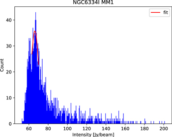
Figure 1. An example of the intensity histogram obtained for the NGC 6334I MM1 region. The mean and the standard deviation were obtained through Gaussian fitting to subtract the continuum emission.
Download figure:
Standard image High-resolution imageAfter subtracting continuum emission in the (u, v) domain, spectral cubes are obtained by the CASA task tclean by applying natural weighting. We also create continuum emission maps with tclean. We show examples of continuum maps in Figure 2, which are created from the spectral window of Band 5, whose center frequency of 203.050 GHz. These continuum maps are used to estimate the hydrogen column densities in the following section. With the CASA task imfit, we performed Gaussian fitting on the continuum peak positions, where we extract the spectra. We create the continuum emission maps and continuum-free spectra through the CASA task immoment.
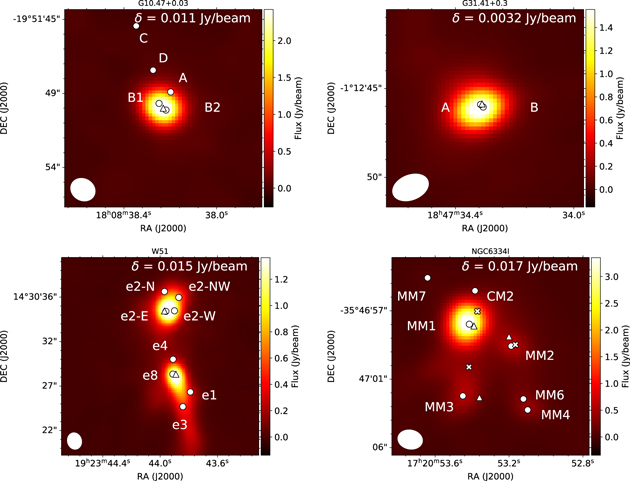
Figure 2. The continuum emission maps created in the spectral window of Band 5, whose center frequency is 203.050 GHz and bandwidth is 0.938 GHz. The spatial scale of 1'' corresponds to a physical distance of 1.3 × 10³, 8.5 × 10³, 3.8 × 10³, and 5.4 × 10³ au, respectively, for NGC 6334I, G10.47+0.03, G31.41+0.3, and W51. The circles represent the positions of previously detected continuum emission. The triangles depict the positions where we extracted the spectra. For NGC 6334I, We show the position observed by Bøgelund et al. (2019). The circles denotes the previously detected continuum peaks. We extracted the spectra from the positions shown by triangles. For detailed information of each source, see the captions in Figures 4–6.
Download figure:
Standard image High-resolution image3. Results
3.1. Spatial Distributions
We show the continuum emission maps and the contamination-free transitions in Figures 2 through 6. Their upper energy levels are shown on the lower right of each figure. Using the CASA task imfit, we performed Gaussian fitting of the peaks of integrated intensity to determine the FWHMs of the source sizes. These source sizes are converted to physical sizes considering the distances to the sources. We summarize our results in Table 4. We note that some species show different excitation temperatures and velocities, suggesting the existence of unresolved spatial components. Therefore, our abundances should be regarded as the average of the unresolved components. Though we discuss the molecular ratios with this limitation in this article, future high-resolution mapping would improve their accuracy.
Table 4. The Coordinates and Deconvolved FWHM Source Sizes
| Source and Transition | α(J2000) | δ(J2000) | Energy Level (K) | Source Size (arcsecond) | Physical Size (×10−3 pc) |
|---|---|---|---|---|---|
| NGC 6334I MM1 | |||||
| continuum | 17:20:53.42 | −35:46:57.8 | 1.88 (±0.10) × 1.23 (±0.12) | 11.8 (±0.6) × 7.7 (±0.8) | |
| CH3OH 133 A− → 132 A+ | 17:20:53.38 | −35:46:58.4 | 261 | 7.7 (±0.3) × 2.95 (±0.12) | 48.6 (±1.9) × 18.6 (±0.8) |
| CH3OH 40 A+ → 30 A+ | 17:20:53.39 | −35:46:58.05 | 23 | 5.57 (±0.17) × 2.76 (±0.09) | 35.1 (±1.0) × 17.4 (±0.6) |
| CH2NH 30,3 → 20,2 | 17:20:53.42 | −35:46:57.91 | 18 | 2.04 (±0.08) × 1.82 (±0.09) | 12.9 (±0.5) × 11.5 (±0.6) |
| CH2NH 32,2 → 22,1 | 17:20:53.42 | −35:46:57.86 | 50 | 1.84 (±0.04) × 1.32 (±0.05) | 11.6 (±0.3) × 8.3 (±0.3) |
| CH2NH 41,3 → 40,4 | 17:20:53.41 | −35:46:58.16 | 40 | 2.85 (±0.08) × 1.81 (±0.07) | 18.0 (±0.5) × 11.4 (±0.5) |
| CH2NH 32,1 → 22,0 | 17:20:53.42 | −35:46:57.81 | 50 | 1.85 (±0.04) × 1.36 (±0.04) | 11.7 (±0.2) × 8.6 (±0.3) |
| CH2NH 71,6 → 70,7 | 17:20:53.42 | −35:46:57.94 | 97 | 2.44 (±0.06) × 1.67 (±0.05) | 15.4 (±0.4) × 10.5 (±0.3) |
| CH2NH 32,1 → 41,4 | 17:20:53.42 | −35:46:57.88 | 50 | 2.07 (±0.05) × 1.3 (±0.04) | 13.1 (±0.3) × 8.2 (±0.3) |
| CH3NH2 42E1-1 → 141E1+1 | 17:20:53.42 | −35:46:57.78 | 0 | 2.43 (±0.07) × 1.58 (±0.07) | 15.3(±0.4) × 10.0 (±0.4) |
| CH3NH2 162B2 → 161B1 | 17:20:53.42 | −35:46:58.05 | 305 | 2.82 (±0.07) × 1.51 (±0.06) | 17.7 (±0.4) × 9.5 (±0.4) |
| CH3NH2 122E1-1 → 121E1+1 | 17:20:53.42 | −35:46:58.0 | 182 | 2.3 (±0.05) × 1.3 (±0.05) | 14.5 (±0.3) × 8.2 (±0.3) |
| CH3NH2 42A1 → 41A2 | 17:20:53.42 | −35:46:57.91 | 37 | 1.86 (±0.06) × 1.28 (±0.06) | 11.7 (±0.4) × 8.0 (±0.4) |
| CH3NH2 41E2+1 → 30E2+1 | 17:20:53.42 | −35:46:57.8 | 26 | 1.85 (±0.08) × 1.42 (±0.08) | 11.6 (±0.5) × 8.9 (±0.5) |
| CH3NH2 41B1 → 30B2 | 17:20:53.41 | −35:46:57.95 | 26 | 2.66 (±0.11) × 1.51 (±0.08) | 16.7 (±0.7) × 9.5 (±0.5) |
| CH3NH2 80B1 → 71B2 | 17:20:53.39 | −35:46:57.64 | 77 | 3.64 (±0.21) × 2.7 (±0.17) | 23.0 (±1.4) × 17.0 (±1.1) |
| CH3NH2 41E1+1 → 30E1+1 | 17:20:53.42 | −35:46:57.87 | 26 | 2.6 (±0.08) × 1.62 (±0.06) | 16.4 (±0.5) × 10.2 (±0.4) |
| CH3NH2 92E1+1 → 91E1-1 | 17:20:53.41 | −35:46:57.78 | 112 | 2.63 (±0.15) × 1.75 (±0.11) | 16.6 (±0.9) × 11.0 (±0.7) |
| NGC 6334I MM2 | |||||
| continuum | 17:20:53.20 | −35:46:59.2 | 2.59 (±0.20) × 1.69 (±0.16) | 16.3 (±1.3) × 10.6 (±1.0) | |
| CH3OH 133 A− → 132 A+ | 17:20:53.2 | −35:46:58.64 | 261 | 3.5 (±0.22) × 2.3 (±0.15) | 22.0 (±1.4) × 14.5 (±1.0) |
| CH3OH 40 A+ → 30 A+ | 17:20:53.22 | −35:46:58.49 | 23 | 4.76 (±0.24) × 2.86 (±0.15) | 30.0 (±1.5) × 18.0 (±0.9) |
| CH2NH 30,3 → 20,2 | 17:20:53.41 | −35:46:57.66 | 18 | 3.99 (±0.18) × 0.67 (±0.09) | 25.2(±1.1) × 4.2 (±0.5) |
| CH2NH 32,2 → 22,1 | 17:20:53.42 | −35:46:57.86 | 50 | 1.84 (±0.06) × 1.34 (±0.07) | 11.6 (±0.4) × 8.45 (±0.4) |
| CH2NH 32,1 → 22,0 | 17:20:53.29 | −35:46:57.71 | 50 | 2.72 (±0.28) × 1.14 (±0.15) | 17.1 (±1.8) × 7.2 (±1.0) |
| CH2NH 71,6 → 70,7 | 17:20:53.22 | −35:46:57.99 | 97 | 2.21 (±0.14) × 1.25 (±0.1) | 13.9 (±0.9) × 7.9 (±0.6) |
| CH3NH2 122E1-1 → 121E1+1 | 17:20:53.42 | −35:46:57.98 | 182 | 2.20 (±0.07) × 1.31 (±0.07) | 13.9 (±0.4) × 8.26 (±0.4) |
| CH3NH2 32B1 → 31B2 | 17:20:53.21 | −35:46:58.25 | 29 | 1.47 (±0.49) × 0.76 (±0.4) | 9.3 (±3.1) × 4.8 (±2.5) |
| CH3NH2 42A1 → 41A2 | 17:20:53.11 | −35:47:0.04 | 37 | 4.08 (±2.16) × 1.17 (±0.63) | 25.7 (±13.6) × 7.4 (±4.0) |
| CH3NH2 41B1 → 30B2 | 17:20:53.18 | −35:46:58.9 | 26 | 2.13 (±0.25) × 0.84 (±0.21) | 13.4 (±1.6) × 5.3 (±1.3) |
| CH3NH2 41E1+1 → 30E1+1 | 17:20:53.19 | −35:46:58.76 | 26 | 2.43 (±0.32) × 0.9 (±0.24) | 15.3 (±2.0) × 5.7 (±1.5) |
| NGC 6334I MM3 | |||||
| continuum | 17:20:53.44 | −35:47:02.1 | 3.29 (±0.19) × 2.16 (±0.11) | 20.7 (±1.2) × 13.6 (±0.7) | |
| CH3OH 40 A+ → 30 A+ | 17:20:53.35 | −35:47:03.1 | 23.2 | 1.54 (±0.29) × 0.66 (±0.53) | 9.7 (±1.8) × 4.2 (±3.3) |
| CH3OH 133 A− → 132 A+ | 17:20:53.36 | −35:47:02.7 | 261.0 | 2.04 (±0.29) × 0.81 (±0.27) | 12.9 (±1.8) × 5.1 (±1.7) |
| G10.47+0.03 | |||||
| continuum | 18:08:38.23 | –19:51:50.4 | 1.83 (±0.03) × 1.71 (±0.03) | 75.4 (±1.2) × 70.4(±1.2) | |
| CH3OH 133 A− → 132 A+ | 18:08:38.23 | −19:51:50.53 | 261 | 2.14 (±0.12) × 2.0 (±0.12) | 88.4 (±5.0) × 82.3 (±4.9) |
| CH3OH 40 A+ → 30 A+ | 18:08:38.23 | −19:51:50.39 | 23 | 2.57 (±0.1) × 2.36 (±0.09) | 106.0 (±4.1) × 97.2 (±3.8) |
| CH2NH 30,3 → 20,2 | 18:08:38.24 | −19:51:50.46 | 18 | 1.94 (±0.08) × 1.67 (±0.07) | 79.8 (±3.3) × 68.8 (±2.9) |
| CH2NH 32,2 → 22,1 | 18:08:38.24 | −19:51:50.49 | 50 | 1.43 (±0.03) × 1.19 (±0.02) | 59.1 (±1.3) × 49.0 (±1.0) |
| CH2NH 41,3 → 40,4 | 18:08:38.24 | −19:51:50.46 | 40 | 1.62 (±0.04) × 1.46 (±0.04) | 66.6 (±1.7) × 60.1 (±1.5) |
| CH3NH2 32B1 → 31B2 | 18:08:38.24 | −19:51:50.53 | 29 | 1.56 (±0.06) × 1.3 (±0.05) | 64.2 (±2.5) × 53.8 (±1.9) |
| CH3NH2 111B2 → 102B1 | 18:08:38.22 | −19:51:50.54 | 146 | 1.9 (±0.09) × 1.5 (±0.08) | 78.2 (±3.9) × 61.8 (±3.4) |
| CH3NH2 41E2+1 → 30E2+1 | 18:08:38.26 | −19:51:50.48 | 26 | 1.36 (±0.06) × 0.8 (±0.06) | 56.0 (±2.4) × 32.9 (±2.6) |
| CH3NH2 41B1 → 30B2 | 18:08:38.23 | −19:51:50.64 | 26 | 1.65 (±0.06) × 1.32 (±0.05) | 67.9 (±2.5) × 54.5 (±2.1) |
| CH3NH2 80B1 → 71B2 | 18:08:38.23 | −19:51:50.56 | 77 | 2.15 (±0.13) × 1.89 (±0.11) | 88.4 (±5.2) × 77.7 (±4.5) |
| G31.41+0.03 | |||||
| continuum | 18:47:34.32 | –01:12:46.01 | 1.36 (±0.07) × 1.21 (±0.07) | 24.7 (±1.2) × 22.1 (±1.2) | |
| CH3OH 133 A− → 132 A+ | 18:47:34.31 | −01:12:46.12 | 261 | 2.02 (±0.05) × 1.9 (±0.05) | 36.6 (±0.9) × 34.5 (±0.9) |
| CH3OH 40 A+ → 30 A+ | 18:47:34.29 | −01:12:46.74 | 23 | 4.61 (±0.38) × 3.64 (±0.34) | 83.9 (±6.8) × 66.3 (±6.2) |
| CH2NH 30,3 → 20,2 | 18:47:34.3 | −01:12:46.2 | 18 | 1.82 (±0.09) × 1.69 (±0.12) | 33.1 (±1.7) × 30.7 (±2.1) |
| CH2NH 32,2 → 22,1 | 18:47:34.31 | −01:12:46.21 | 50 | 1.34 (±0.01) × 1.15 (±0.02) | 24.3 (±0.3) × 20.9 (±0.4) |
| CH2NH 41,3 → 40,4 | 18:47:34.3 | −01:12:46.18 | 40 | 1.49 (±0.03) × 1.3 (±0.05) | 27.1 (±0.5) × 23.7 (±0.9) |
| CH2NH 32,1 → 22,0 | 18:47:34.31 | −01:12:46.16 | 50 | 1.33 (±0.03) × 1.04 (±0.06) | 24.2 (±0.5) × 18.9 (±1.0) |
| CH2NH 71,6 → 70,7 | 18:47:34.31 | −01:12:46.16 | 97 | 1.53 (±0.03) × 1.27 (±0.03) | 27.7 (±0.5) × 23.1 (±0.5) |
| CH2NH 32,1 → 41,4 | 18:47:34.32 | −01:12:46.09 | 50 | 1.37 (±0.07) × 1.32 (±0.07) | 24.9 (±1.3) × 24.1 (±1.3) |
| CH3NH2 32B1 → 31B2 | 18:47:34.31 | −01:12:46.16 | 29 | 1.18 (±0.06) × 1.06 (±0.07) | 21.5 (±1.0) × 19.3 (±1.2) |
| CH3NH2 41E2+1 → 30E2+1 | 18:47:34.32 | −01:12:46.11 | 26 | 1.19 (±0.05) × 0.98 (±0.06) | 21.6 (±0.8) × 17.8 (±1.0) |
| CH3NH2 41B1 → 30B2 | 18:47:34.32 | −01:12:46.11 | 26 | 1.36 (±0.05) × 1.24 (±0.06) | 24.7 (±0.9) × 22.6 (±1.0) |
| CH3NH2 41E1+1 → 30E1+1 | 18:47:34.32 | −01:12:46.08 | 26 | 1.42 (±0.05) × 1.29 (±0.05) | 25.9 (±0.8) × 23.4 (±0.9) |
| W51 e2 | |||||
| continuum | 19:23:43.94 | +14:30:34.8 | 2.47 (±0.17) × 1.55 (±0.13) | 64.6 (±4.4) × 40.6 (±3.4) | |
| CH3OH 133 A− → 132 A+ | 19:23:43.97 | +14:30:34.57 | 261 | 2.5 (±0.12) × 2.07 (±0.11) | 65.6 (±3.2) × 54.1 (±2.9) |
| CH3OH 40 A+ → 30 A+ | 19:23:43.98 | +14:30:34.61 | 23 | 3.23 (±0.17) × 2.72 (±0.16) | 84.5 (±4.5) × 71.2 (±4.1) |
| CH2NH 30,3 → 20,2 | 19:23:43.97 | +14:30:34.02 | 18 | 3.37 (±0.48) × 1.4 (±0.36) | 88.2 (±12.5) × 36.7 (±9.4) |
| CH2NH 32,2 → 22,1 | 19:23:43.97 | +14:30:34.07 | 50 | 2.01 (±0.32) × 0.68 (±0.33) | 52.7 (±8.5) × 17.7 (±8.7) |
| CH2NH 41,3 → 40,4 | 19:23:43.95 | +14:30:34.61 | 40 | 2.83 (±0.15) × 1.56 (±0.13) | 74.1 (±4.1) × 40.9 (±3.3) |
| CH2NH 32,1 → 22,0 | 19:23:43.96 | +14:30:34.38 | 50 | 2.87 (±0.31) × 1.14 (±0.24) | 75.0 (±8.0) × 29.9 (±6.2) |
| CH2NH 71,6 → 70,7 | 19:23:43.96 | +14:30:34.23 | 97 | 2.06 (±0.16) × 1.08 (±0.14) | 53.8 (±4.1) × 28.3 (±3.6) |
| CH3NH2 122E1-1 → 121E1+1 | 19:23:43.96 | +14:30:34.35 | 182 | 1.16 (±0.12) × 0.71 (±0.15) | 30.3 (±3.0) × 18.6 (±3.9) |
| CH3NH2 32B1 → 31B2 | 19:23:43.94 | +14:30:34.29 | 29 | 1.63 (±0.09) × 0.95 (±0.09) | 42.7 (±2.4) × 24.8 (±2.5) |
| CH3NH2 42A1 → 41A2 | 19:23:43.97 | +14:30:33.94 | 37 | 0.0 (±1.24) × 0.0 (±0.46) | 0.0 (±32.4) × 0.0 (±12.0) |
| CH3NH2 41B1 → 30B2 | 19:23:43.96 | +14:30:34.45 | 26 | 1.45 (±0.06) × 0.96 (±0.06) | 37.9 (±1.5) × 25.1 (±1.6) |
| CH3NH2 41E1+1 → 30E1+1 | 19:23:43.96 | +14:30:34.42 | 26 | 1.66 (±0.04) × 1.3 (±0.04) | 43.4 (±1.2) × 34.0(±1.1) |
| W51 e8 | |||||
| continuum | 19:23:43.89 | +14:30:27.6 | 3.07 (±0.35) × 1.18 (±0.23) | 80.3 (±9.2) × 30.9 (±6.0) | |
| CH3OH 133 A− → 132 A+ | 19:23:43.89 | +14:30:28.11 | 261 | 2.64 (±0.14) × 2.07 (±0.12) | 69.2 (±3.6) × 54.2 (±3.1) |
| CH3OH 40 A+ → 30 A+ | 19:23:43.9 | +14:30:27.87 | 23 | 3.36 (±0.28) × 2.4 (±0.2) | 88.0 (±7.5) × 62.9 (±5.4) |
| CH2NH 30,3 → 20,2 | 19:23:43.89 | +14:30:27.91 | 18 | 1.99 (±0.16) × 1.57 (±0.13) | 52.1 (±4.1) × 41.0 (±3.3) |
| CH2NH 32,2 → 22,1 | 19:23:43.89 | +14:30:27.97 | 50 | 1.55 (±0.08) × 1.1 (±0.07) | 40.6 (±2.1) × 28.8 (±1.7) |
| CH2NH 41,3 → 40,4 | 19:23:43.89 | +14:30:27.95 | 40 | 1.9 (±0.1) × 1.36 (±0.08) | 49.6 (±2.7) × 35.5 (±2.1) |
| CH2NH 32,1 → 22,0 | 19:23:43.89 | +14:30:27.94 | 50 | 1.54 (±0.06) × 1.07 (±0.05) | 40.4 (±1.6) × 28.0 (±1.3) |
| CH2NH 71,6 → 70,7 | 19:23:43.89 | +14:30:28.0 | 97 | 1.59 (±0.05) × 1.09 (±0.04) | 41.6 (±1.2) × 28.4 (±1.0) |
| CH3NH2 32B1 → 31B2 | 19:23:43.89 | +14:30:28.07 | 29 | 1.27 (±0.09) × 1.04 (±0.1) | 33.1 (±2.5) × 27.3 (±2.5) |
| CH3NH2 41E2+1 → 30E2+1 | 19:23:43.9 | +14:30:27.99 | 26 | 1.2 (±0.04) × 0.84 (±0.04) | 31.3 (±1.0) × 21.9 (±1.0) |
| CH3NH2 41B1 → 30B2 | 19:23:43.89 | +14:30:27.94 | 26 | 1.33 (±0.08) × 0.81 (±0.08) | 34.9 (±2.2) × 21.3 (±2.1) |
| CH3NH2 80B1 → 71B2 | 19:23:43.88 | +14:30:27.59 | 77 | 2.44 (±0.13) × 1.36 (±0.09) | 63.8 (±3.5) × 35.7 (±2.5) |
Note. We summarized the coordinates and deconvolved FWHM source sizes of the different transitions, obtained by Gaussian fitting. We selected two transitions for one species with the different upper energy levels. The physical source sizes are calculated using the distances to the sources. CH3NH2 41 B1 →30 B2 transition in W51 e8 is regarded as a point source after the deconvolution.
In NGC 6334I, Hunter et al. (2006) performed mapping observations of 1.3 mm continuum emission with the Submillimeter Array (SMA), and reported the structures named SMA1, SMA2, SMA3, and SMA4. Later, Brogan et al. (2016) carried out mapping with angular resolution as high as 0 17 (220 AU) from 5 cm to 1.3 mm with the Karl G. Jansky Very Large Array (VLA) and ALMA. They found the continuum peaks of MM1, MM2, MM3, MM4, MM6, MM7, MM9, and CM2, where MM1, MM2, MM3, and MM4 respectively correspond to the previously known SMA1, SMA2, SMA3, and SMA4. Of these components, MM1 is known as a dramatic outburst source, associated with 6.7 GHz methanol maser and mid-infrared emission (Hunter et al. 2018, 2021). MM3 is known to be a UCHII region associated with free–free emission (Hunter et al. 2006). Many organic molecules have been reported in MM1 and MM2 (e.g., Walsh et al. 2010; Zernickel et al. 2012; El-Abd et al. 2019).
Our molecular distributions overlap with the positions of MM1, MM2, and MM3. The distributions of the CH3OH transitions extend over ∼10''. This scale is close to the maximum recoverable scale. These maps suggest the existence of these species not only in the hot cores but also in the surrounding warm envelopes. As the results of Gaussian fitting to the compact components, the deconvolved source size for CH3OH is 4''. The source sizes for CH3NH2 and CH2NH are 2'', which correspond to ∼0.02 pc.
Though the previous continuum mapping observations by Brogan et al. (2016) suggested the existence of at least seven cores in MM1, our spatial resolution is not sufficient to resolve such structures. We analyze the molecular abundances assuming that molecular emission fills our synthesized beam. Future higher-resolution mapping observations of CH3OH would enable us to investigate the detailed distributions of CH3OH, CH3NH2, and CH2NH.
Bøgelund et al. (2019) reported the distributions of CH3NH2 and CH2NH in MM1 and MM2 with ALMA Band 7 receivers, which are consistent with our results. We note that the location of the continuum peak position of NGC 6334I MM1 is offset from that of Bøgelund et al. (2019) by about 2''. This difference may arise from the complex structure of this source due to the embedded cores. High-resolution mappings would be helpful to resolve such sources. As the molecular peak positions are close to that of our continuum peak, we extract the spectra of our continuum peak position of MM1 in the analysis of molecular abundance. Though our continuum peak position of MM2 is almost identical with Bøgelund et al. (2019), we find that the molecular peak positions are offset from the continuum peak position by about 1'' (see Figure 3). Since the difference of peak positions of molecules are small compared to the synthesized beam size, we extract the spectra from the peak integrated intensity position of CH3OH 133 A− → 132 A+. The continuum peak position of MM3 is offset to the north by ∼3'' from the molecular peak positions. We extracted the spectra from the peak position of the CH3OH 133 A− → 132 A+ transition.
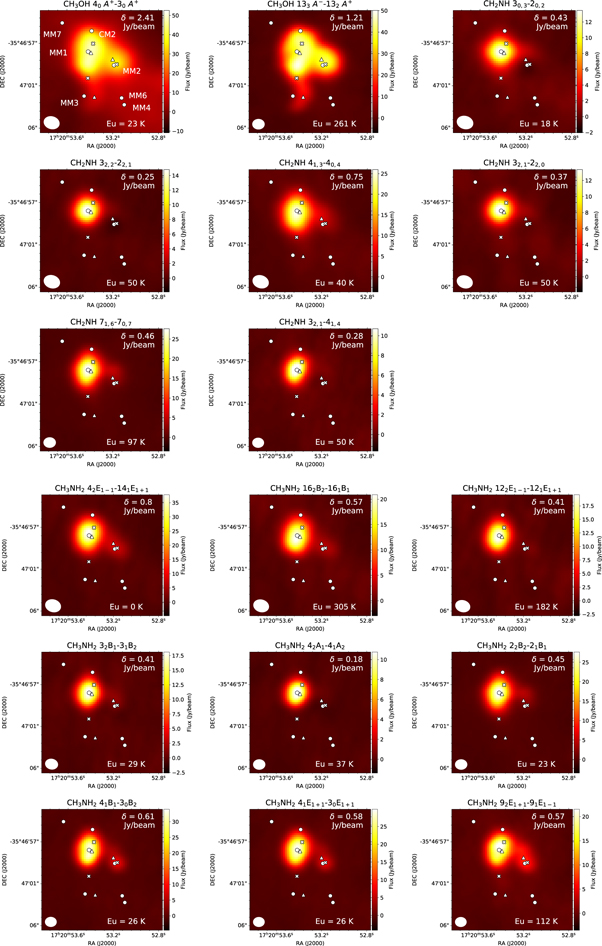
Figure 3. Figures are continued on the next page. The integrated intensity maps of CH3OH, CH3NH2, and CH2NH transitions in NGC 6334I. The rms noise level, δ Jy beam−1, is shown at the top right. The positions of the continuum sources (Hunter et al. 2006; Brogan et al. 2016) are shown by circles. The triangles show the positions of hot cores MM1, MM2, and MM3, where the spectra were extracted. The positions observed by Bøgelund et al. (2019) are marked with Xs. The velocity ranges are from −14.6 to −0.9, from −14.2 to −5.9, and from −13.9 to −0.2 km s−1 for CH3OH, CH3NH2, and CH2NH, respectively. The upper energy level is shown at the bottom left of the figures.
Download figure:
Standard image High-resolution imageG10.47+0.03 is a well-known massive star-forming region associated with several UCHII and HCHII regions. Wood & Churchwell (1989) reported the UCHII regions A, B, and C via 2 and 6 cm mapping with the VLA (see Figure 4). Cesaroni et al. (1998) further resolved component B into HCHII regions B1 and B2 with 1.3 cm VLA observations. They interpreted these sources as face-on rotating disks. The absorption of the NH3(4, 4) transition in these B1 and B2 cores is probably due to molecular outflows originating from HCHII regions. Cesaroni et al. (2010) resolved components A, B1, and B2 with 6, 2, and 1.3 cm continuum emission as well, and newly detected component D with 3.6 cm continuum emission. Cesaroni et al. (2010) also provided evidence of infalling gas toward the embedded cores associated with the outflows. Our maps show that the molecules are distributed around the B1 and B2 positions. In our maps, the distribution of CH3OH 40 A+ → 30 A+ is slightly extended. The source sizes of other CH3OH lines are comparable to this transition and independent of the upper energy level. The typical FWHM source size for the compact components is ∼2'', which corresponds to ∼0.08 pc. As our peak positions of the continuum emission coincide with those of the peaks of molecular emission, we extract the spectra from the peak positions of the continuum emission.
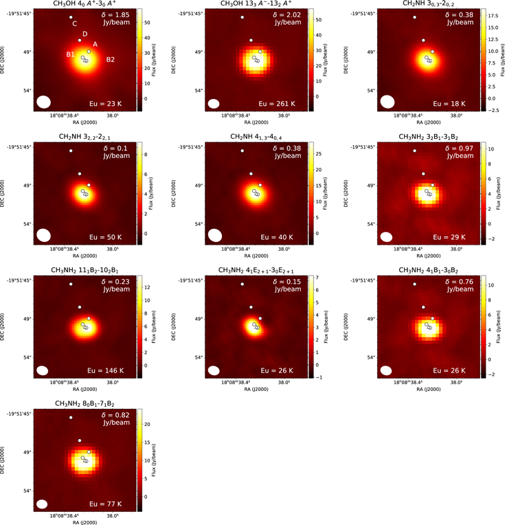
Figure 4. The integrated intensity maps of CH3OH, CH3NH2, and CH2NH transitions in G10.41+0.03. The rms noise level, δ Jy beam−1, is shown at the top right. The positions of continuum sources (Wood & Churchwell 1989; Cesaroni et al. 1998, 2010) are shown by circles. The triangles show the positions of hot cores, where the spectra were extracted. The velocity ranges are from 57.6 to 71.3, from 58.8 to 67.1, and from 62.9 to 76.6 km s−1 for CH3OH, CH3NH2, and CH2NH, respectively. The upper energy level is shown at the bottom left of the figures.
Download figure:
Standard image High-resolution imageG31.41+0.3 is a massive star-forming region similar to G10.47+0.03. Although this source has a UCHII region, the position of the hot molecular core is offset from the UCHII region by about 5'' (Cesaroni et al. 1994), which is outside of Figure 5. Cesaroni et al. (2010) detected weak continuum sources A and B inside the hot molecular core of G31.41+0.3, though we could not distinguish them with our spatial resolution. This continuum emission is thought to originate from a thermal jet rather than UCHII regions. The nondetection of UCHII regions inside the hot molecular core of G31.41+0.3 implies that this source is less evolved than G10.47+0.03 (Cesaroni et al. 2010). Our continuum emission and the molecular distributions extend around the continuum sources A and B. Through Gaussian fitting to the peaks, we found that the typical FWHM source sizes are ∼2'', which corresponds to ∼0.05 pc. Therefore the physical characteristics of the observed region relative to the synthesized source are similar to G10.47+0.03. We extract the spectra from the peak integrated intensity position of CH3NH2, which includes the continuum sources A and B.
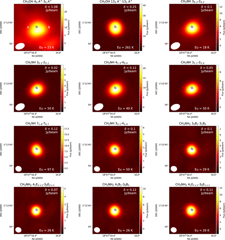
Figure 5. The integrated intensity maps of CH3OH, CH3NH2, and CH2NH transitions in G31.41+0.3. The rms noise level, δ Jy beam−1, is shown at the top right. The positions of continuum sources (Cesaroni et al. 2010) are shown by circles. The triangles show the positions of hot cores, where the spectra were extracted. The velocity ranges are from 85.6 to 99.2, from 89.8 to 98.1, and from 90.8 to 104.5 km s−1 for CH3OH, CH3NH2, and CH2NH, respectively. The upper energy level is shown at the bottom left of the figures.
Download figure:
Standard image High-resolution imageW51 e1/e2 is a well-known protoclustar region, with the UCHII regions e1, e2, e3, e4, and e8 covered in our mapping region (Gaume et al. 1993; Zhang & Ho 1997), as shown in Figure 6. Through the mapping observation of 870 μm dust continuum emission with SMA, Tang et al. (2009) detected the extension of dust ridges northwest of e2 with an overall length of ∼2'', and southwest of e8 with an overall length of ∼3''. They suggest that the gravitational collapse would be slowed down by magnetic fields, affecting the morphology of the source. W51 e2 is the strongest H ii region, which is thought to be powered by an O8-type star (Shi et al. 2010). Shi et al. (2010) performed continuum mapping of W51 e2 at 0.85 and 1.3 mm with ALMA, and at 7 and 13 mm with VLA. They identified the subcores named e2-N, e2-W, e2-E, and e2-NW. The emission from e2-N is free–free emission from the H ii region, while the other continuum emission may be from dust. Of the four sources, e2-E was the only source associated with hydrogen recombination lines (H26α, H53α, and H66α). Goddi et al. (2016) found that e2-E and e2-NW are associated with NH3 and CH3OH emission, respectively, while e2-W is traced by absorption. The detailed structure in e2 is not resolved in our maps. The emission of CH3OH 40 A+ → 30 A+ and CH2NH 30,3 → 20,2 overlap with the dust ridges detected by Tang et al. (2009). The FWHM source sizes of CH3OH and CH2NH are larger than for CH3NH2. The typical FWHM source sizes are ∼3'' for CH3OH and CH2NH, which corresponds to ∼0.08 pc. This physical scale is larger than for NGC 6334I, but comparable to G10.47+0.03 and G31.41+0.3. Our molecular emission peaks are close to the continuum peak positions. Therefore, we extract the spectra from the continuum peak positions, which correspond to W51 e2-E and e8, and hereafter we call W51 e2-E as simply W51 e2.
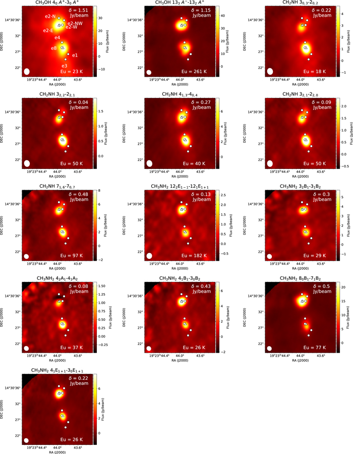
Figure 6. The integrated intensity maps of CH3OH, CH3NH2, and CH2NH transitions in W51 e1/e2. The rms noise level, δ Jy beam−1, is shown at the top right. The positions of continuum sources (Gaume et al. 1993; Shi et al. 2010) are shown by circles. The triangles show the positions of hot cores, where the spectra were extracted. The velocity ranges are from 44.9 to 58.5, from 49.8 to 58.1, and from 47.0 to 60.7 km s−1 for CH3OH, CH3NH2, and CH2NH, respectively. The upper energy level is shown at the bottom left of the figures.
Download figure:
Standard image High-resolution imageGiven our synthesized beam size, the peak positions of the integrated intensities of the different species are close enough for the G10.47+0.03, G31.41+0.3, and W51 e1/e2 regions. On the other hand, the complex spatial morphology of NGC 6334I suggests the existence of unresolved hot cores. In this paper, we do not consider the diversity of the column densities for the unresolved cores. We note that the CH3NH2/CH3OH ratio of this source may change if the cores are sufficiently resolved by future observations. Future higher-resolution observations would be important to obtain more detailed chemical characteristics of these cores.
3.2. Spectra and Analysis
We show the spectra of potentially strong CH2NH and CH3NH2 transitions with black lines in Figure 7 through 12. The CH2NH 71,6 → 70,7 transition at 250.16168 GHz and CH3NH2 22 B2 → 21 B1 transition at 250.1594 GHz are blended with each other.

Figure 7. The observed transitions of CH3NH2 and CH2NH of NGC 6334I MM1 after correcting for Doppler shift. TMB is the brightness temperature. The vertical dotted lines represent the rest-frame frequency. The synthesized spectra obtained by CASSIS overlap the spectra with the red line.
Download figure:
Standard image High-resolution image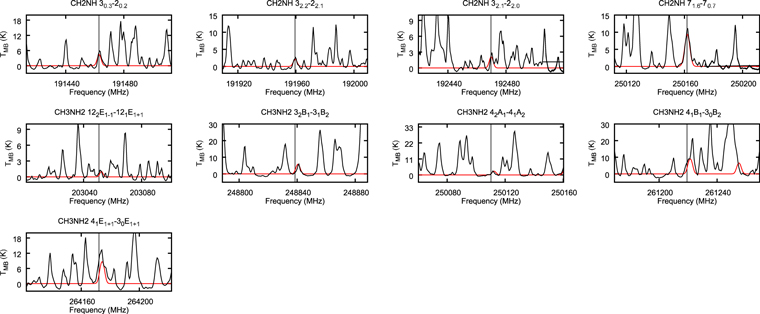
Figure 8. The same as Figure 7 but of NGC 6334I MM2.
Download figure:
Standard image High-resolution image
Figure 9. The same as Figure 7 but of G10.47+0.03.
Download figure:
Standard image High-resolution image
Figure 10. The same as Figure 7 but of G31.41+0.3.
Download figure:
Standard image High-resolution image
Figure 11. The same as Figure 7 but of W51 e2.
Download figure:
Standard image High-resolution image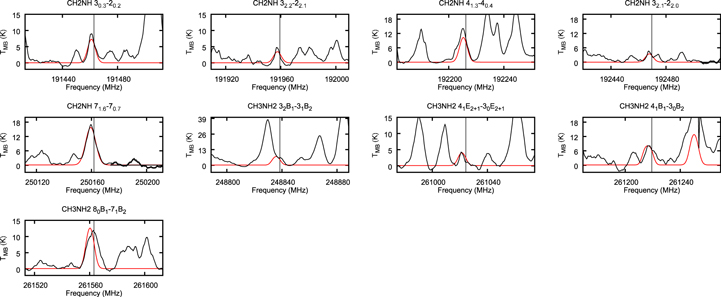
Figure 12. The same as Figure 7 but of W51 e8.
Download figure:
Standard image High-resolution imageWe use the CASSIS line analysis package (Centre d'Analyze Scientifique de Spectres Instrumentaux et Synth'etiques) 6.2 to model the emission and absorption lines with the LTE approximation (Vastel et al. 2015). First of all, we create the best-fit model of CH3OCHO, CH3OCH3, CH3COCH3, C2H3CN, C2H5CN, and NH2CHO to exclude the possibility of contamination. As these COMs are known to be present in typical hot core environments and have rich molecular lines in our observed frequency range, we carefully select contamination-free transitions of CH3OH, CH3NH2, and CH2NH. Then, we performed least-squares fitting with the j thon scripting tool in CASSIS. We simulate the line shape from the given parameters, and the best column densities, excitation temperatures, line widths, and radial velocities are given by minimizing the residuals relative to the observed spectrum. With Markov Chain Monte Carlo methods, the initial values of the parameters are randomly given. We found that 3000 iterations are good enough to obtain the best parameters. The errors were given from the standard deviation of the best-fit parameters. The best-fitted synthesized spectra, including CH3OH, CH3NH2, and CH2NH, are shown overlapping with the observed spectra by the red line in Figures 7 through to 11. The column density of molecular hydrogen is estimated from the continuum emission from the dust in the same way as Hernández-Hernández et al. (2014). In this method, the gas mass is calculated as
where Sν , D, Rd, κν , and Bν (Td) are the flux density, distance to the source, the gas-to-dust ratio, the dust opacity per unit dust mass, and the Planck function at the dust temperature Td, respectively. First, from Ossenkopf & Henning (1994), we use a κν of 2.0 cm2 g−1 at 1.3 mm, which corresponds to 230 GHz. We estimate κν at the other frequencies with the emissivity spectral index of dust of 1.5 as

Then, with an Rd of 100, and using the Rayleigh–Jeans approximation, we estimate the hydrogen column density with the following equation

where θ is the synthesized beam size (radians). In our work, we use the angular resolution of our observations as θ. Assuming that the source is uniformly filled within the beam, we ignore the frequency dependency of the source size. We obtain Sν from the continuum maps (Figure 2), which are created in the procedure of continuum subtraction. We approximate the dust temperature by assuming it to be the excitation temperature of CH3OH. We use all the spectral windows to obtain the mean hydrogen column densities, and the standard deviation of the hydrogen column densities to estimate the errors. As free–free emission is evident in NGC 6334I MM3, we subtract the contribution of free–free emission to estimate the hydrogen column density of this source. Utilizing VLA archival data, Hunter et al. (2006) estimated the fraction of free–free emission at 1.3 mm to be 62% of the total flux of continuum emission. With the caveat that this percentage is deduced from an observation of the 3.6 cm flux density, we multiply the observed flux of continuum emission by 0.62 to take into account the contribution of free–free emission in NGC 6334I MM3. We summarize our results in Table 5.
Table 5. Abundance and Abundance Ratios of CH3OH, CH3NH2, and CH2NH
| Source | CH3NH2/CH3OH obs | N[H2] obs | X[CH3OH] obs | X[CH3NH2] obs | X[CH2NH] obs |
|---|---|---|---|---|---|
| NGC 6334I MM1 | 0.30 ± 0.03 | 7.5 ± 0.5 (24) | 3.6 ± 0.4 (−7) | 1.0 ± 0.1 (−7) | 1.4 ± 0.1 (−8) |
| NGC 6334I MM2 | 0.007 ± 0.0008 | 9.4 ± 0.7 (23) | 1.9 ± 0.1 (−6) | 1.2 ± 0.1 (−8) | 5.5 ± 0.5 (−9) |
| NGC 6334I MM3 | 1.8 ± 0.5 (24) | 3.4 ± 1.1 (−7) | <5.6 (−9) | <8.3 (−10) | |
| G10.47+0.03 | 0.13 ± 0.02 | 2.0 ± 0.2 (24) | 2.3 ± 0.3 (−6) | 2.9 ± 0.3 (−7) | 3.6 ± 0.3 (−8) |
| G31.41+0.3 | 0.16 ± 0.02 | 1.8 ± 0.3 (24) | 6.1 ± 1.3 (−7) | 1.0 ± 0.1 (−7) | 1.9 ± 0.3 (−8) |
| W51 e2 | 0.065 ± 0.006 | 9.1 ± 0.9 (24) | 1.1 ± 0.1 (−7) | 8.6 ± 1.1 (−9) | 1.0 ± 0.1 (−9) |
| W51 e8 | 0.078 ± 0.004 | 4.1 ± 0.3 (24) | 2.9 ± 0.2 (−7) | 1.9 ± 0.1 (−8) | 4.6 ± 0.4 (−9) |
| Previous study | CH3NH2/CH3OH | ||||
| Sgr B2(M)a | 8.0 × 10⁻³ | ||||
| Sgr B2(N)a | 0.03 | ||||
| Sgr B2(N)b | 0.10 | ||||
| NGC 6334I MM1c | (2.5–5.9) × 10−3 | ||||
| NGC 6334I MM2c | (0.9–1.5) × 10−3 | ||||
| NGC 6334I MM3c | (4.8–5.4) × 10−4 | ||||
| IRAS 16293-2422Bd | <5.3 × 10⁻⁵ | ||||
| Garrod fast modele | 0.007 | ||||
| Garrod medium modele | 0.004 | ||||
| Garrod slow modele | 0.001 | ||||
Note. Top: the observed CH3NH2/CH3OH ratio is shown. N[H2] is the column density of H2. X[CH3OH], X[CH3NH2], and X[CH2NH] are, respectively, the fractional abundances of CH3OH, CH3NH2, and CH2NH, compared to the molecular hydrogen column density. Bottom: the CH3NH2/CH3OH ratio from previous studies. References: (a) Belloche et al. (2013), (b) Neill et al. (2014), (c) Bøgelund et al. (2019), (d) Ligterink et al. (2018), and (e) Garrod (2013).
Download table as: ASCIITypeset image
3.3. Column Densities and Abundances
As a result of our fitting, we detected our species of interest in all sources. Especially, we report the first detection of CH3NH2 in G31.41+0.03, W51 e2, and W51 e8. Our column densities and the excitation temperatures of H2, CH3OH, CH3NH2, and CH2NH are summarized in Table 6. In Table 5, we convert the column densities into fractional abundances compared to H2.
Table 6. The Derived Abundances with CASSIS Fitting
| Source | Species | Tex (K) | N (cm−2) | Δv (km s−1) | VLSR (km s−1) |
|---|---|---|---|---|---|
| NGC 6334I MM1 | CH3OH | 224 ± 8 | 2.7 ± 0.3 (18) | 6.7 ± 0.2 | 6.94 ± 0.04 |
| 80 ± 1 | 1.3 ± 0.1 (18) | 4.7 ± 0.1 | 3.71 ± 0.07 | ||
| CH3OCHO | 231 ± 12 | 8.8 ± 0.3 (17) | 4.9 ± 0.1 | 7.20 ± 0.03 | |
| 69 ± 7 | 6.4 ± 1.4 (16) | 4.6 ± 0.3 | 5.59 ± 0.29 | ||
| CH3OCH3 | 119 ± 1 | 1.2 ± 0.1 (18) | 4.7 ± 0.1 | 6.42 ± 0.04 | |
| 54 ± 1 | 1.4 ± 0.6 (16) | 4.0 ± 0.3 | 5.86 ± 0.27 | ||
| C2H5CN | 200 ± 1 | 4.7 ± 0.4 (16) | 4.9 ± 0.3 | 6.88 ± 0.33 | |
| 56 ± 1 | 6.3 ± 1.4 (15) | 4.0 ± 0.1 | 6.12 ± 0.06 | ||
| CH2NH | 274 ± 15 | 1.1 ± 0.1 (17) | 5.7 ± 0.2 | 7.30 ± 0.08 | |
| CH3NH2 | 120 ± 3 | 8 ± 0.4 (17) | 6.1 ± 0.1 | 7.18 ± 0.06 | |
| NGC 6334I MM2 | CH3OH | 218 ± 5 | 1.8 ± 0.1 (18) | 4.2 ± 0.2 | 4.80 ± 0.05 |
| 50 ± 5 | 7.4 ± 1.9 (16) | 5.8 ± 0.7 | 5.30 ± 0.13 | ||
| CH3OCHO | 285 ± 17 | 7.9 ± 0.4 (17) | 3.9 ± 0.1 | 4.88 ± 0.04 | |
| 71 ± 1 | 5.4 ± 0.4 (17) | 2.0 ± 0.1 | 5.25 ± 0.04 | ||
| CH3OCH3 | 167 ± 7 | 1.3 ± 0.1 (17) | 4.5 ± 0.1 | 4.18 ± 0.09 | |
| 79 ± 4 | 2 ± 0.1 (17) | 3.0 ± 0.1 | 5.26 ± 0.06 | ||
| CH2NH | 193 ± 2 | 5.2 ± 0.3 (15) | 5.0 ± 0.1 | 5.73 ± 0.07 | |
| CH3NH2 | 50 ± 1 | 1.2 ± 0.1 (16) | 3.0 ± 0.1 | 3.43 ± 0.16 | |
| NGC 6334I MM3 | CH3OH | 169 ± 47 | 6.2 ± 1.9 (17) | 6.2 ± 0.1 | 8.3 ± 0.10 |
| G10.47+0.03 | CH3OH | 172 ± 11 | 4.6 ± 0.6 (18) | 8.3 ± 0.5 | 65.96 ± 0.10 |
| 67 ± 9 | 2.3 ± 0.7 (17) | 10.0 ± 1.4 | 66.07 ± 0.45 | ||
| CH3OCHO | 185 ± 7 | 6.9 ± 0.3 (17) | 8.1 ± 0.2 | 67.23 ± 0.08 | |
| 53 ± 1 | 4.2 ± 0.7 (16) | 7.2 ± 0.1 | 66.87 ± 0.26 | ||
| CH3OCH3 | 232 ± 17 | 6.2 ± 0.2 (17) | 6.9 ± 0.1 | 66.44 ± 0.13 | |
| 80 ± 3 | 5.6 ± 2.2 (16) | 4.3 ± 0.1 | 61.02 ± 0.84 | ||
| C2H3CN | 227 ± 12 | 2.6 ± 0.3 (17) | 7.0 ± 0.1 | 67.16 ± 0.12 | |
| 93 ± 12 | 4.7 ± 0.2 (17) | 4.6 ± 0.2 | 66.89 ± 0.21 | ||
| C2H5CN | 99 ± 1 | 4.2 ± 0.1 (17) | 6.2 ± 0.1 | 66.88 ± 0.05 | |
| CH2NH | 195 ± 2 | 7.2 ± 0.3 (16) | 8.2 ± 0.5 | 66.83 ± 0.10 | |
| CH3NH2 | 181 ± 8 | 5.9 ± 0.3 (17) | 7.0 ± 0.1 | 67.07 ± 0.14 | |
| 59 ± 2 | 3.4 ± 0.6 (16) | 4.4 ± 0.1 | 67.93 ± 0.21 | ||
| G31.41+0.3 | CH3OH | 249 ± 5 | 1.1 ± 0.2 (18) | 10.6 ± 0.6 | 97.23 ± 0.13 |
| 13 ± 5 | 5 ± 15.3 (15) | 3.7 ± 0.4 | 98.35 ± 0.27 | ||
| CH3OCHO | 227 ± 12 | 6.9 ± 0.4 (17) | 7.2 ± 0.1 | 97.76 ± 0.06 | |
| CH3OCH3 | 167 ± 31 | 4.5 ± 0.3 (17) | 8.8 ± 0.2 | 97.50 ± 0.08 | |
| C2H3CN | 217 ± 4 | 2.5 ± 0.1 (16) | 9.5 ± 0.2 | 97.02 ± 0.23 | |
| C2H5CN | 239 ± 9 | 3.6 ± 0.1 (16) | 9.1 ± 0.2 | 97.20 ± 0.09 | |
| CH2NH | 176 ± 11 | 3.5 ± 0.2 (16) | 8.1 ± 0.2 | 97.23 ± 0.11 | |
| CH3NH2 | 94 ± 3 | 1.8 ± 0.1 (17) | 8.9 ± 0.1 | 96.53 ± 0.08 | |
| W51 e8 | CH3OH | 250 ± 13 | 1 ± 0.1 (18) | 9.1 ± 0.4 | 57.45 ± 0.06 |
| 33 ± 1 | 9.8 ± 2.0 (15) | 5.8 ± 0.4 | 56.34 ± 0.12 | ||
| CH3OCHO | 229 ± 9 | 2.1 ± 0.2 (17) | 8.6 ± 0.2 | 57.51 ± 0.14 | |
| 21 ± 1 | 1.9 ± 0.3 (17) | 5.1 ± 0.2 | 54.70 ± 0.60 | ||
| CH3OCH3 | 174 ± 7 | 1.3 ± 0.1 (17) | 8.7 ± 0.1 | 58.31 ± 0.08 | |
| C2H3CN | 250 ± 6 | 2.5 ± 0.1 (16) | 8.7 ± 0.2 | 59.90 ± 0.12 | |
| CH2NH | 199 ± 8 | 1.9 ± 0.1 (16) | 10.1 ± 0.2 | 59.71 ± 0.09 | |
| CH3NH2 | 87 ± 4 | 7.8 ± 0.3 (16) | 7.6 ± 0.2 | 59.99 ± 0.08 | |
| 16 ± 1 | 3.4 ± 1.1 (15) | 8.6 ± 0.1 | 61.10 ± 0.16 | ||
| W51 e2 | CH3OH | 244 ± 17 | 1.2 ± 0.1 (18) | 9.8 ± 0.1 | 55.38 ± 0.12 |
| 67 ± 9 | 7.2 ± 2.3 (17) | 6.7 ± 0.9 | 54.02 ± 0.88 | ||
| CH3OCHO | 200 ± 15 | 5.2 ± 0.2 (17) | 5.3 ± 1.0 | 55.31 ± 0.11 | |
| 65 ± 11 | 2 ± 0.5 (17) | 9.5 ± 1.4 | 54.63 ± 1.54 | ||
| CH3OCH3 | 150 ± 13 | 4.2 ± 0.3 (17) | 8.5 ± 0.2 | 55.27 ± 0.34 | |
| 30 ± 1 | 2.4 ± 7.2 (15) | 5.4 ± 0.1 | 56.73 ± 0.13 | ||
| C2H5CN | 209 ± 3 | 2.2 ± 0.1 (16) | 9.2 ± 0.1 | 55.90 ± 0.34 | |
| 30 ± 1 | 2.1 ± 3.5 (15) | 4.8 ± 0.1 | 57.30 ± 0.10 | ||
| CH2NH | 203 ± 1 | 1 ± 0.1 (16) | 5.2 ± 0.1 | 56.97 ± 0.03 | |
| CH3NH2 | 74 ± 1 | 7.9 ± 0.7 (16) | 6.5 ± 0.7 | 54.24 ± 0.26 |
Note. The column densities, the excitation temperatures, the line widths, and the radial velocities derived by CASSIS fitting. a (b) means a × 10b.
Download table as: ASCIITypeset image
The CH3NH2 abundances of G10.47+0.03, NGC 6334I MM1, and G31.41+0.3 show higher values of ∼1.0 × 10⁻⁷. On the other hand, NGC 6634I MM3 has low abundance of CH3NH2 and a high abundance of CH3OH (3.4 × 10⁻⁷). Since the Gaussian-fitted source sizes of CH3OH are larger than those of CH2NH and CH3NH2, the abundances of N-bearing species may have been underestimated relative to those of O-bearing species in Suzuki et al. (2018) due to beam dilution. The excitation temperature of CH3NH2 in G10.47+0.03 is 172 K, which is much higher than that reported by Ohishi et al. (2019), where the excitation temperature was ∼46 K. The low excitation temperature of CH3NH2 given by Ohishi et al. (2019) implies that CH2NH is in the extended envelope component structure surrounding the hot core. In Ohishi et al. (2019), the beam size of the NRO 45 m telescope was ∼20'', being larger than our maximum recoverable scale of ∼10''. Such a component would be unresolved with our interferometric observation since we did not use the ALMA Compact Array (ACA). In this case, it would be difficult to compare the column densities with those of Ohishi et al. (2019) in this study. Since we could not detect CH2NH and CH3NH2 in the NGC 6334I MM3 region, we estimate the upper limit of the column densities using all transitions covered in our observations with an excitation temperature of 169 K, corresponding to that of CH3OH, and a line width of 6.0 km s−1. Through line simulation with CASSIS, we get an upper limit to the column density of 1.0 × 1016 cm−2, which corresponds to a fractional abundance of 5.6 × 10⁻⁹. For CH2NH, the upper limit of the column density for NGC 6334I MM3 is 1.5 × 1015 cm−2, which corresponds to a fractional abundance of 8.3 × 10⁻¹⁰. The three cores in the NGC 6334I region, MM1, MM2, and MM3, are chemically interesting regions, as Bøgelund et al. (2019) reported that the abundances of CH3NH2 and CH2NH differ by orders of magnitude in them. Our column densities of CH2NH and CH3NH2 agree with Bøgelund et al. (2019) within a factor of three. Since our observed position of NGC 6334I is offset by about 2'' compared to Bøgelund et al. (2019), this difference would not be surprising. In addition, our receiver setup enables us to obtain the column density of CH3OH in MM1, MM2, and MM3 simultaneously. The low CH3NH2/CH3OH ratios of NGC 6334I MM2 and MM3 clearly show the depletion of only N-bearing species.
Finally, we show the spectra of the hydrogen recombination line H39β in Figure 13, which we could observe simultaneously in this work. While this line is evident in NGC 6334I MM3, it is very weak for the other sources. This result suggests the physical evolution of NGC 6334I MM1 and MM2 is in an early phase, as the ionization of hydrogen atoms by the stellar radiation field is not dominant.
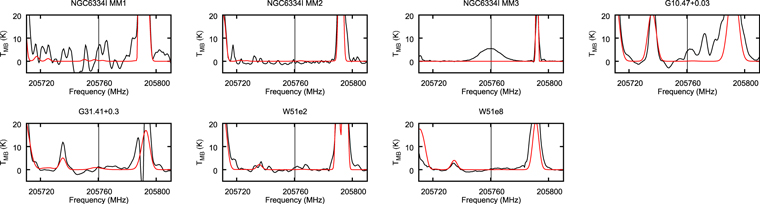
Figure 13. The spectra of the hydrogen recombination line H39β. The vertical dotted line represents the rest-frame frequency of this line, 205.760337 GHz. Other details are the same as Figure 7.
Download figure:
Standard image High-resolution image4. Comparison with Chemical Modeling
4.1. Chemical Model and its Parameters
In this section, we evaluate our observational results using the chemical model described in Suzuki et al. (2018). In this previous work, we utilized the three-phase chemical model NAUTILUS (Ruaud et al. 2016, and references therein). We used the gas-phase chemical network kida.uva.2014
10
(Wakelam et al. 2015), and the grain surface reactions in Garrod (2013). With these reaction sets, we updated the formation process of CH3NH2. We added the hydrogenation processes of HCN on the grain surface (HCN + 2H → H2CN and H2CN + 2H → CH3NH2), resulting in an increase of CH3NH2 abundance. In total, 489 species composed of 13 elements (H, He, C, N, O, Si, S, Fe, Na, Mg, Cl, P, and F) were included. We used the canonical cosmic-ray ionization rate of 1.3 × 10⁻¹⁷ s−1. To simulate the physical conditions in hot cores, we assumed two stages for the physical model, where freefall collapse is followed by a dynamically static warm-up. The cold collapse phase started from  = 3 × 103 cm−3 to a final postcollapse density of
  = 2 × 107 cm−3. In this phase, we use the formula of Nejad et al. (1990), where factor B controls the timescale of this phase. While B = 1 corresponds to freefall collapse, a smaller value of B describes the effects of turbulent, thermal, or magnetic resistance. In our model, the factor B only slows down the collapsing phase, without affecting any physical evolution during the warm-up phase. The factor B was set to unity, which corresponds to the case of freefall. The increase in visual extinction during collapse leads to a minimum dust-grain temperature of 8 K, followed by a warm-up to 400 K; during this phase, the gas and dust temperatures are assumed to be well coupled. The gas density during the warm-up phase is fixed to be the final gas density of the freefall collapse (i.e.,
  = 2 × 107 cm−3). For the timescale, we employed the fast warm-up model since this model was prepared for the physical evolution of high-mass star-forming regions (Garrod 2013). The timescale for the warm-up phase is 7.12 × 10⁴ yr. After this time, the temperature remains fixed to the maximum value of 400 K. Since we achieved the best agreement after the end of the warm-up phase in Suzuki et al. (2018), we discuss the comparison beyond 7.12 × 10⁴ yr.
We test the parameter dependencies of our model by running our model with different cosmic-ray ionization rates, ζ. While the canonical value for ζ is 1.3 × 10⁻¹⁷ s−1, Barger & Garrod (2020) suggested higher values for ζ up to 2 × 10⁻¹⁶ s−1 to explain their observations of chemical species. In Models A, B, and C, we set ζ to be 1.3 × 10⁻¹⁷, 5.2 × 10⁻¹⁷, and 1.3 × 10⁻¹⁶ s−1, respectively (see Table 7 for the detailed parameters). We present the time evolution of the fractional abundances of CH3OH, CH3NH2, and CH2NH in Figure 14. Cosmic rays efficiently destroy molecules when ζ is large. With an ζ of 1.3 × 10⁻¹⁷ s−1, it takes ∼1 × 10⁶ yr after the beginning of warm-up to explain the observed CH3OH and CH3NH2. On the other hand, this timescale decreases to less than 2 × 10⁵ yr with an ζ of 1.3 × 10⁻¹⁶ and 5.2 × 10⁻¹⁷ s−1. Since the weak hydrogen recombination lines (Figure 13) suggest the younger evolutional phase, Models B and C would be reasonable. Considering that the typical timescale for hot cores to have a detectable UCHII region is ∼105 yr (Churchwell 2002), ζ should be larger than 5.2 × 10⁻¹⁷ s−1. Hereafter, we fix ζ to 5.2 × 10⁻¹⁷ s−1 since this is the best value of ζ for NGC 6334I IRS1 (Barger & Garrod 2020).

Figure 14. The results of the chemical model with the different cosmic-ray ionization rates of ζ = 1.3 × 10⁻¹⁷, 5.2 × 10⁻¹⁷, and 1.3 × 10⁻¹⁶ s−1, respectively, for Models A, B, and C. The simulated fractional abundances, X, of CH3OH, CH3NH2, and CH2NH in the gas phase are shown by red, blue, and green solid lines, respectively. The dotted line represents the sum of the fractional abundances in the grain mantle and on the grain surface. The region where the model can reproduce the observed values within a factor of 10 is indicated by red and blue for CH3OH and CH3NH2, respectively, and the overlapping region is painted by gray.
Download figure:
Standard image High-resolution imageTable 7. The Parameters of the Chemical Model
| Model | ζ (s−1) | T (K) | n (cm s−3) | B | Warm-up Speed |
|---|---|---|---|---|---|
| A | 1.3 (−17) | 400 | 1 (7) | 1 | fast |
| B | 5.2 (−17) | 400 | 1 (7) | 1 | fast |
| C | 1.3 (−16) | 400 | 1 (7) | 1 | fast |
| D | 5.2 (−17) | 200 | 1 (7) | 1 | fast |
| E | 5.2 (−17) | 600 | 1 (7) | 1 | fast |
| F | 5.2 (−17) | 400 | 1 (6) | 1 | fast |
| G | 5.2 (−17) | 400 | 1 (8) | 1 | fast |
| H | 5.2 (−17) | 400 | 1 (7) | 0.1 | fast |
| I | 5.2 (−17) | 400 | 1 (7) | 0.2 | fast |
| J | 5.2 (−17) | 400 | 1 (7) | 0.7 | fast |
| K | 5.2 (−17) | 400 | 1 (7) | 1 | medium |
Note. The parameters of our chemical models. The parameters ζ, T, and n, respectively, represent the cosmic-ray ionization rate, the peak temperature, and the peak density. B controls the timescale of the collapsing phase (Nejad et al. 1990). We use the same warm-up models of Garrod (2013).
Download table as: ASCIITypeset image
The other free parameters of our simulations are the factor B, peak temperature, peak density, and timescale of the warm-up phase. Based on Model B, we prepared physical models with different collapsing speeds, temperatures, densities, and warm-up timescales, as summarized in Table 7. We determine the peak temperature from the comparison with the theoretical model. As our sources are located at a different distances, the temperatures of the observed regions are different from source to source. We use the temperature profiles in Nomura & Millar (2004), which were predicted by a detailed radiative transfer model together with observations of the spectral energy distributions of hot molecular cores. Then, considering the distances to the sources and our synthesized beam size of ∼1'', the typical temperatures in our observations would be ∼500, ∼200, ∼300, and ∼300 K for NGC 6334I, G10.41+0.03, G31.41+0.3, and W51 e1/e2, respectively. Our synthesized beam would cover the hot regions where the frozen species would sufficiently sublimate. Therefore, in Models D and E, the peak temperature is changed to 200 and 600 K, respectively. In Models F and G, the final gas densities are 1 × 10⁶ and 1 × 108 cm−3, respectively. We note that we used the same initial density in Models F and G. In Models H, I, and J, the factor B is set to 0.7, 0.2, and 0.1, respectively, to control the collapsing speed. We use the medium models in Garrod (2013) for Model K.
4.2. Simulation Results of the Abundances and CH3NH2/CH3OH Ratio
As an example, we show our simulation results in Figure 15 with Model B. The simulated fractional abundances of CH3OH, CH3NH2, and CH2NH, compared to the total proton density in the gas phase and on grains (sum of the molecular abundances in the grain mantle and on the grain surface) are shown by solid and dotted lines, respectively. In the comparison between the simulated and observed abundances, we multiply the observed abundances by a factor of 2 since the observed abundances are the relative abundances compared to hydrogen molecules (two protons). A time of zero years corresponds to the beginning of the warm-up phase. The left panel of Figure 15 represents the fractional abundances until 1 × 10⁶ yr after the beginning of the warm-up phase. As we discussed in the previous studies, CH2NH is efficiently formed in the gas-phase reaction CH3 + NH → CH2NH + H, while CH3NH2 is built on grain surfaces via successive hydrogenation processes of HCN (Suzuki et al. 2016, 2018). When the grain surface temperature gets high enough, these species sublimate from grains, leading to a sudden increase of the gas-phase abundances. The sublimation of CH3NH2 happens at ∼6.2 × 10⁴ yr, when the dust temperature is ∼130 K, while the sublimation of CH3OH occurs when the dust temperature is ∼110 K due to the smaller binding energy. Since CH3NH2 is frozen before 6.2 × 10⁴ yr, the results before this age would be not meaningful.

Figure 15. The results of Model B (the standard model). (a) The simulated fractional abundances, X, of CH3OH, CH3NH2, and CH2NH in the gas phase are shown by red, blue, and green solid lines, respectively. The vertical axis represent the ages of the core since the beginning of warm-up. We present the CH3NH2 abundance predicted by Model B', where we switch off the series of hydrogenation processes of HCN and CH2NH to form CH3NH2, by the purple line. The dotted line represent the sum of the fractional abundances in the grain mantles and on the grain surfaces. (b) The gas-phase CH3NH2/CH3OH ratio. With horizontal lines, we compare the observed CH3NH2/CH3OH ratio of our sources. The abundance ratios are calculated from Table 5.
Download figure:
Standard image High-resolution imageFirst of all, we compare Model B with the fast warm-up model of Garrod (2013). Our peak fractional abundances of CH3OH, CH3NH2, and CH2NH in the gas phase during the warm-up phase are 3.2 × 10⁻⁵, 3.4 × 10⁻⁶, and 2.3 × 10⁻⁶, respectively. Garrod (2013) reported the peak abundances of CH3OH, CH3NH2, and CH2NH in the gas phase to be 1.1 × 10⁻⁵, 8.0 × 10⁻⁸, and 1.1 × 10⁻⁸, respectively. Hence, there is a disagreement in the CH3NH2 and CH2NH abundances. For CH2NH, the disagreement is due to the update of the gas-phase formation process of CH2NH with kida.uva.2014 (see Suzuki et al. 2016 for details). For CH3NH2, the difference is due to the inclusion of the hydrogenation processes of HCN and CH2NH. We prepare Model B' where we switch off the series of hydrogenation processes to form CH3NH2 from Model B. The simulated fractional abundances from Models B and B' are compared in Figure 15. The peak abundance of CH3NH2 from Model B' is 4.3 × 10⁻⁸, which agrees with Garrod (2013).
We show the CH3NH2/CH3OH ratio from Model B in the right panel of Figure 15. Both CH3OH and CH3NH2 are formed on grains through the hydrogenation process during the warm-up phase and destroyed simultaneously in the gas phase after sublimation by reactive radicals, ions, and cosmic rays. However, there is a time variation in the CH3NH2/CH3OH ratio. The CH3NH2/CH3OH ratio is ∼0.01 at first, and it increases to 0.05 at ∼3 × 10⁵ yr. This increase is due to the formation of CH3NH2 in the gas phase through the following series of reactions: (1) CH3 + + NH3 → CH3NH3 + and then (2) CH3NH3 + + e− → CH3NH2 + H. After ∼3 × 10⁵ yr, the CH3NH2/CH3OH ratio drops dramatically due the formation of CH3OH in the gas phase. First, the abundances of the ionized species increase due to cosmic rays. Then, CH3OH forms through the recombination processes of these ions form CH3OH. For example, CH3OH4 + + e− → CH3 + CH3OH and CH3COCH4 + + e− → CH3CO + HCO + H, then H + CH3OCO → CH3OH + CO. Though these reactions have to be considered with caution due to the lack of reliable measurements of the reaction rates, as we will see, the agreement with the observed abundances is achieved mainly before 3 × 10⁵ yr.
We compare the observed fractional abundances of CH3OH, CH3NH2, and CH2NH with the simulated fractional abundances derived from the chemical model. The errors of the observed fluxes during the calibration and the continuum subtraction should be ∼10% (ALMA technical handbook). On the other hand, the errors of the chemical model result should be propagated from thousands of reactions with the uncertain reaction rates along the time evolution. Hence, the errors of the chemical model are more significant. Since it is difficult to constrain the errors of the chemical model, we employ a criterion for the comparison as being within a factor of 10, which is often used for comparisons with simulations in previous studies (e.g., Wakelam et al. 2015).
In Figure 16, we compare the simulated fractional abundances of CH2NH from Models B, D, and E, where the peak temperatures are 400, 200, and 600 K, respectively. All models show a fractional abundance of CH2NH higher than 1 × 10⁻⁷ after sublimation. We also display the observed CH2NH abundances in blue, indicating the chemical models overproduce CH2NH. As discussed in Suzuki et al. (2016), CH2NH is efficiently produced by the reaction CH3 + NH. The formation rate of CH2NH from radicals is well investigated (see Hébrard et al. 2012; Loison et al. 2014; Wakelam et al. 2015 for details), and therefore this overproduction would not be due to the wrong formation rate. Our model considers the formation and destruction chemistry of CH2NH from the KIDA database. However, the destruction reactions of CH2NH are largely dominated by ion–molecule reactions, which are mostly efficient in low-temperature environments. Therefore, additional high-temperature theoretical and experimental data exploring the possible neutral–neutral and radical–neutral destruction reactions of CH2NH may provide a closer agreement with the observations.

Figure 16. The fractional abundance of CH2NH in the gas phase predicted by Models B, D, and E. These models have peak temperatures of 400, 200, and 600 K, respectively. The blue area represents the region where the observed CH2NH abundances can be explained.
Download figure:
Standard image High-resolution imageIn Table 8, we summarize the ages where our models can explain the observed fractional abundances and the CH3NH2/CH3OH ratio for each source. In this table, we set a criterion that the simulated fractional abundances of CH3OH and CH3NH2 are within a factor of 10 compared to the observed abundances. The molecular ratio of CH3NH2/CH3OH would be a more valid indicator as the uncertainty of the H2 column densities disappears. We compare the observed CH3NH2/CH3OH ratios with the simulations considering the error propagation of the observations. As a result, we can successfully explain the observation results with certain parameter sets, except for NGC 6334I MM3, where the CH3NH2 abundance was too low to detect.
Table 8. The Simulated Ages of the Hot Cores (×105 yr)
| Source | B | D | E | F | G | H | I | J | K |
|---|---|---|---|---|---|---|---|---|---|
| NGC 6334I MM1 | x | x | x | x | x | x | x | 1.56–2.26 | x |
| NGC 6334I MM2 | 0.63–1.68 | 0.63–1.78 | 0.63–1.68 | 0.62–1.96 | 0.64–1.62 | x | x | 0.63–1.26 | 2.4–2.7 |
| G10.47+0.03 | 0.63–1.96 | 0.63–2.1 | 0.63–1.94 | 0.63–2.28 | 0.64–1.9 | x | x | 0.63–1.46 | 2.1–3.13 |
| G31.41+0.3 | 1.56–2.32 | 1.64–2.4 | 1.64–2.26 | x | 1.54–2.16 | x | x | x | 2.82–3.56 |
| W51 e2 | 1.52–1.7 | 1.58–1.8 | 1.48–1.78 | 1.58–3.28 | 1.5–1.52 | x | 0.63 | x | x |
| W51 e8 | x | x | x | 1.42–2.02 | x | x | 0.63 | x | x |
| NGC 6334I MM1 | x | x | x | x | x | x | x | x | x |
| NGC 6334I MM2 | 0.64–1.7 | 0.63–1.68 | 0.63–1.68 | 0.62–1.96 | 0.64–1.62 | x | x | 0.65–1.38 | 2.1–2.7 |
| G10.47+0.03 | 0.65–1.02 | 0.64–1.96 | 0.64–1.94 | 0.63–2.18 | 0.65–1.9 | x | x | x | 2.1–3.12 |
| G31.41+0.3 | x | 1.94–2.34 | 2–2.26 | x | 1.9–2.28 | x | x | x | 3.42–3.57 |
| W51 e2 | 1.38–2.72 | 1.38–2.08 | 1.36–2.1 | 1.6–3.28 | 1.32–2.04 | x | 0.65–1.02 | x | 2.5–3.74 |
| W51 e8 | 2.3–2.56 | 1.24–1.46 | 1.22–1.56 | 1.42–2.52 | 1.18–1.48 | x | 0.66–0.78 | x | 2.3–2.5 |
Note. The ages of hot cores (×105 yr) needed to explain the simulated fractional abundances of CH3OH and CH3NH2, and the CH3NH2/CH3OH ratio within a factor of 10 with the different physical models. The upper row shows a comparison with a model with a hydrogenation reaction, and the lower row shows a comparison with a model without a hydrogenation reaction. The symbol "x" shows that the model is unable to explain the observation.
Download table as: ASCIITypeset image
In Figure 17, we show the time evolution of the fractional abundances of CH3NH2 and CH3OH, and their ratio for the different Models D, E, F, G, H, I, J, and K. Though the overall trends of chemical evolution are similar to Model B, we can see that the molecular abundances are influenced by the physical environment. Especially, as we see in Models H, I, and J, the gravitational collapse speed controlled by B shows the largest effect on the CH3NH2/CH3OH ratio. We also note that the observation results of NGC 6334I MM1, where CH3NH2 is especially abundant compared to CH3OH, are reproduced only with Model J, where B is set to 0.7. Models H and J, where the smaller B slows down the collapse phase, the models overproduced the CH3NH2 abundance compared to the observations. Since the low binding energy of HCN is higher than for CO, a small value of B leads to a higher abundance of HCN on the grains. As a result, a large amount of CH3NH2 is built through the series of hydrogenation processes of HCN. This difference may give us important insight for CH3NH2 chemistry. Though Models H and I likely show too large CH3NH2 abundances, Model J where B = 0.7 shows a reasonably high CH3NH2/CH3OH ratio. These results suggest that the differences of CH3NH2 abundances could be due to the different collapsing speeds of the core before the birth of the star.

Download figure:
Standard image High-resolution image
Figure 17. Figures are continued on the next page. Same as Figure 15, but for the other models.
Download figure:
Standard image High-resolution image
NGC 6334I MM3 is an interesting source where the fractional abundance of CH3OH is exceptionally high, while CH3NH2 is not detected. We observed a strong hydrogen recombination line, H39β, in NGC 6334I MM3, suggesting a later phase of evolution when cosmic rays destroy gas-phase species. Though our simulation results after ∼3 × 10⁵ yr can explain the low observed CH3NH2 abundance of NGC 6334I MM3, the simulated gas-phase CH3OH abundance is too low to explain the observed abundance at such phase. Our current model may not be suitable to explain the later phase of the chemical evolution due to a lack of reliable gas-phase chemistry of COMs.
To see the importance of the hydrogenation processes for the formation of CH3NH2, we compare the observed CH3NH2/CH3OH ratios with Garrod (2013), where the hydrogenation processes of HCN and CH2NH are not included. As we see in Table 5, the peak abundance ratio of CH3NH2/CH3OH is 0.007 with the fast warm-up model, which is the highest among the three models in Garrod (2013). These values are too low to explain our observations. In addition, we run the chemical model turning off the hydrogenation processes for HCN and CH2NH to see the importance of the hydrogenation processes. Our results are summarized in the lower part of Table 8. While we can explain the observed abundances and ratios for some sources based on the selected conditions and ages, we could not find any condition to reproduce the chemistry of NGC 6334I MM1, where CH3NH2 is the most abundant. With the caveat that we still have uncertain rate coefficients of the gas-phase reactions, these results suggest the importance of the hydrogenation processes of HCN and CH2NH for the formation of CH3NH2.
Our conclusion that CH3NH2 is built through the successive hydrogenation processes of HCN is different from that of Bøgelund et al. (2019). In Bøgelund et al. (2019), the authors observed NGC 6334I and derived the CH3NH2 column densities to be 2.7 × 10¹⁷, 6.2 × 10¹⁶, and 3.0 × 1015 cm−2 for MM1, MM2, and MM3, respectively. With these column densities, they obtained that the CH3NH2/CH3OH ratio ranges from ∼5 × 10⁻³ to ∼5 × 10⁻⁴, which agrees with the peak abundance ratio from the fast warm-up model in Garrod (2013) within a factor of 5. Therefore they suggested that CH3NH2 is built via a recombination process of radical species (CH3 + NH2). Their very low CH3NH2/CH3OH ratio for the NGC 6334I region is contrary to our result. Since our CH3NH2 column densities of the NGC 6334I region agree with Bøgelund et al. (2019), this disagreement comes from the CH3OH column densities.
We believe our CH3OH column densities are more reliable for a few reasons. First, Bøgelund et al. (2019) observed only one transition of the CH3OH molecule, which would lead to uncertainty of the CH3OH abundance. Second, if we apply their observational results and assume a CH3NH2 column density of 2.7 × 1017 cm−2 and a CH3NH2/CH3OH ratio of 1 × 10⁻³, the CH3OH column density should be 2.7 × 1020 cm−2. This surprisingly high CH3OH column density is not consistent with the previous studies. The column density of CH3OH can be roughly estimated from the previous observation by a single dish telescope. Ikeda et al. (2001) found that the CH3OH column density of NGC 6334I was 3.4 × 1016 cm−2 under the assumption of the source size being 20''. Our mapping result suggests that the source size of CH3OH is ∼5'' in the NGC 6334I region. Then, the CH3OH column density is estimated to be 3.4 × 1016 × (20''/5'')2 = 5.4 × 1017 cm−2. Therefore, the column density of CH3OH used in Bøgelund et al. (2019) appears to be overestimated. The column density of 5.4 × 1017 cm−2 rather agrees with our CH3OH column densities of the NGC 6334I region.
4.3. Comparison with Other Sources
Belloche et al. (2013) and Neill et al. (2014) investigated the CH3NH2 and CH3OH abundances of Sgr B2 (M) and (N). According to these studies, the CH3NH2/CH3OH ratios of Sgr B2 (N) are 0.03 and 0.1, respectively. This difference would come from the smaller beam size of Neill et al. (2014) compared to that of Belloche et al. (2013). The CH3NH2/CH3OH ratio of 0.1 is close to our values for NGC 6334I MM2 and G31.41+0.3. The CH3NH2/CH3OH ratios for NGC 6334I MM1 and W51 e2 are higher than that of Sgr B2. On the other hand, the small value of CH3NH2/CH3OH for Sgr B2(M) is close to that of NGC 6334I MM3. The similarity of Sgr B2(M) with NGC 6334I MM3, and of Sgr B2(N) with NGC 6334I MM1 and MM2 could be due to the fact that Sgr B2(M) is highly dominated by H ii regions, while Sgr B2(N) is more dominated by dust emission (Schmiedeke et al. 2016; Sánchez-Monge et al. 2017).
Pagani et al. (2017) reported the CH3NH2 column density of the Orion KL hot core to be 1 × 1016 cm−2. The CH3OH column density of the Orion KL-W region is reported in Peng et al. (2012). Their CH3OH contour map suggests that the CH3OH abundance at the position of the hot core would be close to the position of the KL-W region. In this case, the CH3OH column density is 9.2 × 1017 cm−2. Therefore we obtain a CH3NH2/CH3OH ratio of 0.011 for the Orion KL hot core, which is similar to that of NGC 6334I MM3.
Finally, we note that we performed this survey of CH2NH-rich sources reported in Suzuki et al. (2016). Therefore our source samples may be biased toward N-bearing species-rich sources. Further CH3NH2 surveys of other hot cores would be essential to reveal a more general picture of hot core chemistry. CH3NH2 surveys of low-mass protostars are also an interesting topic. For hot corinos, the CH3NH2/CH3OH ratio was investigated only for IRAS16293-2422. The CH3NH2/CH3OH ratio in this source is less than 5.3 × 10⁻⁵, which is dramatically lower than our result. Such a difference could be due to the higher binding energy of CH3NH2. Therefore the source size of CH3NH2 may be much smaller for low-mass stars, which require extremely high angular resolutions.
5. Conclusions
The main results of this paper are summarized as follows:
- 1.We performed a survey of CH3NH2, CH2NH, and CH3OH of the sources NGC 6334I, G10.47+0.03, G31.41+0.3, and W51 e1/e2 with ALMA. We resolved hot core components, MM1, MM2, and MM3 in NGC 6334I region, and e2 and e8 covered in our mapping of the W51 e1/e2 region. In total, we analyzed the molecular abundances of seven hot cores. CH3NH2, CH2NH, and CH3OH are detected for all sources except for NGC 6334I MM3, where CH3NH2 was not detected.
- 2.We obtained the excitation temperatures and column densities of CH3NH2, CH2NH, and CH3OH by employing CASSIS fitting. The CH3NH2 abundances were obtained for G31.41+0.03, W51 e2, and W51 e8 for the first time. NGC 6334I is an especially CH3NH2-rich source with a column density of 1.5 × 1018 cm−2. For the other sources, the column densities of CH3NH2 are typically ∼1017 cm−2, but less than 1 × 1016 cm−2 for NGC 6334I MM3.
- 3.The observed fractional abundances relative to H2 for CH3OH, CH3NH2, and CH2NH are, respectively, ∼10−8, ∼10−8, and ∼10−9. We obtained a CH3NH2/CH3OH ratio between 0.008 and 1.0. NGC 6334I MM3 exhibits an extremely low CH3NH2/CH2NH ratio of <0.002, similar to that seen in the Orion KL hot core and in Sgr B2 (M). It is possible that our source selection may be biased to N-bearing molecule-rich sources. The extension of this survey to an unbiased selection of sources would be important to expand further our knowledge of prebiotic chemistry in dense cores.
- 4.Through a chemical model, we found satisfactory agreement of the fractional abundances of CH3OH and CH3NH2. On the other hand, our model overpredicts the CH2NH abundance. The discrepancy may be due to the omission of destruction processes for CH2NH.
- 5.Our model suggests that the CH3NH2/CH3OH ratio is sensitive to the efficiency of the hydrogenation process to HCN. A high observed CH3NH2/CH3OH ratio suggests the importance of the grain surface hydrogenation processes of HCN and CH2NH to form CH3NH2. We note that the very small CH3NH2/CH3OH ratio of NGC 6334I MM3 is not explained by our chemical model. A detailed discussion for this source is deferred to a future paper.
Acknowledgments
This paper makes use of the following ALMA data: ADS/JAO ALMA#2017.1.01248.S. ALMA is a partnership of ESO (representing its member states), NSF (USA), and NINS (Japan), together with NRC (Canada), MOST and ASIAA (Taiwan), and KASI (Republic of Korea), in cooperation with the Republic of Chile. The Joint ALMA Observatory is operated by ESO, AUI/NRAO, and NAOJ. The National Radio Astronomy Observatory is a facility of the National Science Foundation operated under cooperative agreement by Associated Universities, Inc. This study was supported by the Astrobiology Program of National Institutes of Natural Sciences (NINS) and by the JSPS Kakenhi grant Nos. 19K03936, 19H05069, and 19K14753. L.M. acknowledges the financial support of DAE and DST-SERB research grants (SRG/2021/002116 and MTR/2021/000864) of the Government of India. This research was carried out in part at the Jet Propulsion Laboratory, which is operated by the California Institute of Technology under a contract with the National Aeronautics and Space Administration (80NM0018D0004). K.T. acknowledges support from NAOJ ALMA Scientific Research grant Nos. 2022-22B and Grants-in-Aid for Scientific Research (KAKENHI) of Japan Society for the Promotion of Science (JSPS; grant Nos. JP21H00049 and JP21K13962).
Software: CASA (v5.1.1; McMullin et al. 2007).
Appendix
We summarize the potentially strong molecular lines at our observed frequencies in Table 9. The parameters of the CH3OH, CH3NH2, and CH2NH molecular lines are obtained from the JPL catalog (Ilyushin et al. 2005; Xu et al. 2008; Dore et al. 2010, and references therein).
Table 9. The Observed Transitions
| Species | Frequency (MHz) | Quantum Number | → | Quantum Number | Eu (K) | Sμ2 (D2) | ||||
|---|---|---|---|---|---|---|---|---|---|---|

|

|

| → | J'' | Ka'' | Γ'' | ||||
| CH3OH | 191,732.99 | 6 | 3 | E | → | 7 | 2 | E | 96.5 | 1.4 |
| 191,810.50 | 4 | 1 | A+ | → | 3 | 1 | A+ | 37.6 | 3.0 | |
| 193,415.33 | 4 | 0 | E | → | 3 | 0 | E | 36.3 | 3.2 | |
| 193,441.61 | 4 | −1 | E | → | 3 | −1 | E | 28.8 | 3.0 | |
| 193,454.37 | 4 | 0 | A+ | → | 3 | 0 | A+ | 23.2 | 3.2 | |
| 193,471.43 | 4 | 3 | A+ | → | 3 | 3 | A+ | 73.0 | 1.4 | |
| 193,471.54 | 4 | 3 | A− | → | 3 | 3 | A− | 73.0 | 1.4 | |
| 193,474.42 | 4 | 3 | E | → | 3 | 3 | E | 70.9 | 1.4 | |
| 193,488.05 | 4 | 2 | A− | → | 3 | 2 | A− | 60.9 | 2.4 | |
| 193,488.96 | 4 | −3 | E | → | 3 | −3 | E | 85.9 | 1.4 | |
| 193,506.57 | 4 | 1 | E | → | 3 | 1 | E | 44.3 | 3.1 | |
| 193,510.75 | 4 | 2 | A+ | → | 3 | 2 | A+ | 60.9 | 2.4 | |
| 193,511.23 | 4 | −2 | E | → | 3 | −2 | E | 49.1 | 2.4 | |
| 193,511.34 | 4 | 2 | E | → | 3 | 2 | E | 45.5 | 2.4 | |
| 205,791.23 | 1 | 1 | A+ | → | 2 | 0 | A+ | 16.8 | 1.0 | |
| 247,611.04 | 18 | 3 | A− | → | 18 | 2 | A+ | 446.6 | 17.4 | |
| 247,967.93 | 23 | 1 | E | → | 23 | 0 | E | 661.4 | 11.7 | |
| 248,885.48 | 16 | 3 | A− | → | 16 | 2 | A+ | 365.4 | 15.3 | |
| 249,192.86 | 16 | −3 | E | → | 15 | −4 | E | 378.3 | 4.7 | |
| 249,419.90 | 15 | 3 | A− | → | 15 | 2 | A+ | 328.3 | 14.3 | |
| 249,443.34 | 7 | 4 | A− | → | 8 | 3 | A− | 145.3 | 1.2 | |
| 249,451.89 | 7 | 4 | A+ | → | 8 | 3 | A+ | 145.3 | 1.2 | |
| 250,291.13 | 13 | 3 | A− | → | 13 | 2 | A+ | 261.0 | 12.3 | |
| 250,507.02 | 11 | 0 | A+ | → | 10 | 1 | A+ | 153.1 | 10.6 | |
| 261,805.74 | 2 | 1 | E | → | 1 | 0 | E | 28.0 | 1.3 | |

|

|

| → | J'' | Ka'' | Kb'' | ||||
| CH2NH | 191,462.82 | 3 | 0 | 3 | → | 2 | 0 | 2 | 18.4 | 15.8 |
| 191,959.30 | 3 | 2 | 2 | → | 2 | 2 | 1 | 49.9 | 8.8 | |
| 192,212.32 | 4 | 1 | 3 | → | 4 | 0 | 4 | 39.8 | 29.3 | |
| 192,469.59 | 3 | 2 | 1 | → | 2 | 2 | 0 | 50.0 | 8.8 | |
| 250,161.68 | 7 | 1 | 6 | → | 7 | 0 | 7 | 97.2 | 41.5 | |
| 263,986.06 | 3 | 2 | 1 | → | 4 | 1 | 4 | 50.0 | 2.3 | |

|

|

| → | J'' | Ka'' | Γ'' | ||||
| CH3NH2 | 192,622.39 | 14 | 2 | E1−1 | → | 14 | 1 | E1+1 | 239.0 | 142.4 |
| 193,795.82 | 16 | 2 | B2 | → | 16 | 1 | B1 | 305.3 | 187.0 | |
| 202,791.86 | 3 | 1 | E2−1 | → | 2 | 0 | E2+1 | 16.7 | 3.8 | |
| 203,050.98 | 12 | 2 | E1−1 | → | 12 | 1 | E1+1 | 181.6 | 103.5 | |
| 203,096.32 | 16 | 2 | E1+1 | → | 16 | 1 | E1+1 | 305.9 | 7.7 | |
| 248,838.50 | 3 | 2 | B1 | → | 3 | 1 | B2 | 28.9 | 27.8 | |
| 249,527.26 | 10 | 5 | E2+1 | → | 11 | 4 | E2+1 | 214.8 | 6.0 | |
| 250,110.22 | 4 | 2 | A1 | → | 4 | 1 | A2 | 37.4 | 12.3 | |
| 250,159.40 | 2 | 2 | B2 | → | 2 | 1 | B1 | 22.6 | 15.8 | |
| 250,255.53 | 5 | 2 | E1+1 | → | 5 | 1 | E1−1 | 47.9 | 15.0 | |
| 250,398.51 | 12 | 1 | E1−1 | → | 11 | 2 | E1+1 | 168.6 | 7.8 | |
| 260,963.40 | 11 | 1 | B2 | → | 10 | 2 | B1 | 145.9 | 47.3 | |
| 261,024.31 | 4 | 1 | E2+1 | → | 3 | 0 | E2+1 | 25.9 | 12.5 | |
| 261,219.28 | 4 | 1 | B1 | → | 3 | 0 | B2 | 25.6 | 47.1 | |
| 261,252.83 | 6 | 2 | B1 | → | 6 | 1 | B2 | 60.9 | 53.7 | |
| 261,562.18 | 8 | 0 | B1 | → | 7 | 1 | B2 | 76.8 | 58.6 | |
| 264,172.18 | 4 | 1 | E1+1 | → | 3 | 0 | E1+1 | 25.9 | 44.0 | |
| 264,457.13 | 9 | 2 | E1+1 | → | 9 | 1 | E1−1 | 111.8 | 40.4 | |
| 264,752.35 | 7 | 2 | B2 | → | 7 | 1 | B1 | 75.8 | 60.8 | |
Note. The observed transitions of CH3NH2, CH2NH, and CH3OH. The data were taken from Xu et al. (2008) for CH3OH, Ilyushin et al. (2005) for CH3NH2, and taken from the Spectral Line Atlas of Interstellar Molecules (SLAIM) for CH2NH. Eu represents the energy of the upper state level, while Sμ2 shows the product of the intrinsic line strength and the square of the permanent dipole moment.
The quantum numbers of the CH3OH transitions are described by J, ± Ka, and Γ. For transitions with Γ = A, the Γ is associated with a "+" or "−" sign to represent the parity. On the other hand, Γ = E1 and E2 are presented by the identical alphabet of Γ = E, but denoted by the positive and negative sign of K, respectively, due to the absence of a parity entry.
CH2NH is a simple asymmetric top with all atoms being on a simple plane, and the transitions are described using labels J, Ka, and Kc. Our fitting considers the hyperfine structure of CH2NH.
The transitions of CH3NH2 are labeled by the irreducible representation of torsion, inversion, and rotation Γ, with its states of labeled with A1, A2, B1, B2, E1±1, and E2±1 (Ilyushin & Lovas 2007). The selection rules are Γ = A1 ↔ A2, B1 ↔ B2, E1±1 ↔ E1±1, and E2±1 ↔ E2±1. The symmetry levels have nuclear spin statistical weights of 1 for the A1, A2, and E2 states and 3 for the B1, B2, and E1 components. Our fitting does not consider the hyperfine structures of CH3NH2. According to the splatalogue catalog, the typical frequency separation is less than 100 kHz, which is smaller than our spectral resolution. Therefore they are clearly blended and the summation of the line strengths for all hyperfine structures is reasonable.