


Abstract
New evidence based on Cassini magnetic field and plasma data has revealed that the discovery of Titan outside Saturn's magnetosphere during the T96 flyby on 2013 December 1 was the result of the impact of two consecutive interplanetary coronal mass ejections (ICMEs) that left the Sun in 2013 early November and interacted with the moon and the planet. We study the dynamic evolution of Saturn's magnetopause and bow shock, which evidences a magnetospheric compression from late November 28 to December 4 (at least), under prevailing solar wind dynamic pressures of 0.16–0.3 nPa. During this interval, transient disturbances associated with the two ICMEs are observed, allowing for the identification of their magnetic structures. By analyzing the magnetic field direction, and the pressure balance in Titan's induced magnetosphere, we show that Cassini finds Saturn's moon embedded in the second ICME after being swept by its interplanetary shock and amid a shower of solar energetic particles that may have caused dramatic changes in the moon's lower ionosphere. Analyzing a list of Saturn's bow shock crossings during 2004–2016, we find that the magnetospheric compression needed for Titan to be in the supersonic solar wind can be generally associated with the presence of an ICME or a corotating interaction region. This leads to the conclusion that Titan would rarely face the pristine solar wind, but would rather interact with transient solar structures under extreme space weather conditions.
Export citation and abstract BibTeX RIS

Original content from this work may be used under the terms of the Creative Commons Attribution 4.0 licence. Any further distribution of this work must maintain attribution to the author(s) and the title of the work, journal citation and DOI.
1. Introduction
Solar activity determines plasma conditions throughout the heliosphere. In particular, the occurrence of coronal mass ejections (CMEs) is strongly modulated by the solar cycle with frequencies increasing around the solar maximum (Webb & Howard 1994; Lamy et al. 2019). CMEs consist of large amounts of plasma and magnetic flux that erupt from the solar corona and sail through the interplanetary space (Webb & Howard 2012; Scolini et al. 2022). After an initial accelerating phase in the inner corona (Patsourakos et al. 2010), CMEs propagate in a self-similar way, conserving their magnetic structure (Subramanian et al. 2014; Vršnak et al. 2019). In the interplanetary medium, the traveling CMEs are known as interplanetary CMEs (ICMEs). Near the Sun, slow ICMEs are usually accelerated by the ambient solar wind, while fast ICMEs are decelerated (Gopalswamy et al. 2000; Vršnak & Žic 2007). From about 1 au, ICMEs' propagation speeds can be assumed to be fairly constant (Hoang et al. 2007; Reiner et al. 2007). The magnetic structure of ICMEs can be either that of a complex ejecta (Burlaga et al. 2001) or that of a flux rope (Burlaga et al. 1981). The latter is known as a "magnetic cloud" and is characterized by enhanced magnetic field strength, a smooth and large rotation of the magnetic field vector, and low proton temperature (∼104 K). In addition, fast ICMEs can drive interplanetary shocks that are the predominant drivers of intense geomagnetic storms (e.g., Zhang et al. 2007; Echer et al. 2008), and are separated from the ejecta/cloud by a sheath of compressed, heated solar wind plasma (Richardson & Cane 2010). Interplanetary shocks at fast ICMEs are usually preceded by fluxes of suprathermal protons, heavier ions, and electrons, known as solar energetic particles (SEPs).
Though ICMEs have been extensively studied near 1 au, very few studies have focused on the evolution and magnetic structure of ICMEs in the outer heliosphere (e.g., Burlaga et al. 2001; Witasse et al. 2017; Echer 2019; Palmerio et al. 2021). Planetary missions allow us to sense solar wind conditions at different heliocentric distances. ICME structures can be identified in situ using a number of signatures based on magnetic field, plasma, compositional, and energetic particle data (e.g., Alexander et al. 2006). However, not all spacecraft have dedicated plasma instruments and they might not monitor the solar wind continuously. In these cases, extreme solar wind conditions can still be inferred from measuring indirect signatures of ICMEs such as variations in the flux of Galactic cosmic rays (GCRs) (e.g., Roussos et al. 2018). GCRs are mainly protons with energies above hundreds of MeV to 1 GeV that are accelerated at astrophysical sources. It has been shown that GCRs can present short-term variations, called Forbush decreases (FDs) (Lockwood 1971), that consist of a fast decrease of GCR flux intensity followed by an exponential recovery. FDs are caused by deflections of GCRs as a result of enhanced magnetic fluxes associated with the ICME passage. An advantage of GCRs, as well as of SEPs, is that these energetic particles can penetrate into some planetary magnetospheres and so can be detected even when the spacecraft is not in the solar wind (e.g., Roussos et al. 2018). This is true at least for magnetospheric configurations such as those of Saturn and Jupiter, where weakening field strengths in the equatorial current sheet enhance energetic ions' access to deeper lengths compared to what a purely dipolar configuration would allow (Selesnick 2002; Kotova et al. 2019).
Saturn's (equatorial radius RS = 60,268 km) magnetosphere, the second largest in the solar system, is characterized by a rapidly rotating, nearly axisymmetric magnetic dipole (Gurnett et al. 2005; Dougherty et al. 2018). The strong centrifugal force, together with the mass loading and outward radial transport of heavy ions from the moon Enceladus and the planet's rings, results in the formation of a sub-corotating magnetodisk confined toward the planet's magnetic equator (Achilleos et al. 2015; Szego et al. 2015). Saturn's magnetodisk consists of a ≳2 RS thick central current sheet that separates the magnetospheric northern and southern lobes. The current sheet is a high plasma beta region, with weak, southward magnetic fields. In the northern and southern lobes, magnetic fields are comparatively stronger and point radially away from and toward the planet, respectively. The lobes also show a significantly lower plasma beta. Saturn's magnetopause (MP) is generally close to the locus of balance between the magnetospheric thermal and magnetic pressure and the solar wind dynamic pressure (Sorba et al. 2017; Hardy et al. 2019, 2020), and has an average standoff distance between 22 and 27 RS, following a bimodal distribution (Achilleos et al. 2008). Meanwhile, Saturn's bow shock (BS) average standoff distance is around 25 RS (Masters et al. 2008).
Titan (radius RT = 2575 km) is Saturn's major moon and the only one in the solar system with a dense, optically thick atmosphere (Hörst 2017, and references therein). Titan is also characterized by the absence of a global, intrinsic magnetic field (Ness et al. 1982). As a result, the moon's ionized atmosphere interacts directly with the external plasma. This results in the formation of an induced magnetosphere and leads to the escape of ionospheric particles (Bertucci 2021, and references therein). The magnetic morphology of an induced magnetosphere depends on the direction of the external flow and magnetic field. As the flow approaches the ionosphere on the ram side, the field increases in magnitude (pileup), and the frozen-in magnetic field lines drape around the obstacle defining an induced magnetic tail on the downstream side. If the cross-flow component of the background magnetic field changes, the geometry of the induced magnetosphere follows (Alfvén 1957). The onset of the magnetic field pileup and draping occurs at the induced magnetospheric boundary (IMB), a plasma layer that marks the outer limit of the induced magnetosphere and separates the local from the external plasma (Bertucci et al. 2011). On the ram side, the region behind the IMB—referred to as the magnetic pileup region or MPR—is where the strongest pileup and magnetic pressure are found. If the external flow is supersonic, a BS forms around the IMB with a magnetosheath region between them.
Titan orbits Saturn at an average distance of 20.2 RS. Under typical solar wind conditions, the moon's orbit fits completely inside the Kronian magnetosphere. This means Titan mostly encounters Saturn's partially corotating magnetospheric flow (Thomsen 2013) and interacts with it in a submagnetosonic and sub-Alfvénic regime (Arridge et al. 2011). During periods of enhanced solar wind pressure, Titan has been observed outside the Kronian MP and within the magnetosheath plasma (e.g., Bertucci et al. 2008; Edberg et al. 2013). The strong impact of Saturn's magnetospheric variability on Titan's plasma environment has been broadly studied (e.g., Kabanovic et al. 2017), but little is known about its response to solar wind drivers. Studying the effects of extreme space weather conditions on unmagnetized bodies is especially important to learning about the evolution of their atmospheric structure, as particle escape increases significantly (e.g., Jakosky et al. 2015) and also because a higher rate of solar storms occurred in early solar system history (Wood et al. 2005).
The Cassini mission recorded the activity of Saturn's magnetosphere for a little more than a solar cycle (23 and 24) and nearly half a Saturnian year. Titan was also a primary target, with 126 close flybys. As these flybys were regularly spaced in time, seasonal and solar cycle effects could also be observed. In particular, solar cycle 24 showed a relatively weak maximum around the end of 2013, but a series of large-scale, high-speed ICMEs impacted the Saturn system at that time. Between 2013 November 26 and December 12, Roussos et al. (2018) reported one of the strongest SEP events in their 2004–2016 survey. These SEPs were accelerated by an interplanetary shock, observed by Cassini around November 28 at 21:00 UT, and accompanied by an FD on November 29 between 00:00 and 04:00 UT. Roussos et al. (2018) also reported strong Saturn kilometric radiation (SKR) emissions that extended to low frequencies (∼10 kHz). SKR emissions are radio emissions of a few kHz to 1 MHz emitted by electrons traveling around auroral magnetic field lines and are highly dependent on solar wind conditions, with solar wind dynamic pressure being the main driver of their enhanced activity (Desch 1982; Desch & Rucker 1983; Kurth et al. 2016; Cecconi et al. 2022). The Roussos et al. (2018) observations are of particular interest for the study of Titan plasma interactions, since Cassini's close flyby T96 took place on December 1. Bertucci et al. (2015) reported that during this encounter Titan was interacting with a supersonic solar wind flow, following the detection of Saturn's BS receding past the moon's orbital distance.
To date, the observations during the T96 flyby are the only ones of Titan exposed to the solar wind. However, the space weather implications of the complex plasma context in which the moon was immersed were not yet taken into consideration. In this work, we revisit the T96 observations and go beyond this flyby to investigate the effects of the impact of multiple ICMEs on the Saturn–Titan system. In Section 2 we sum up the data and empirical models used. In Section 3.1, we analyze the dynamics of Saturn's MP and BS prior to and after the T96 flyby and study the degree of compression of Saturn's magnetosphere that allowed for the exposure of Titan to the solar wind. In Section 3.2, we identify the cause of the enhanced solar wind pressure as the impact of two consecutive ICMEs, identify their magnetic structures, and correlate the observed space weather events to their potential solar sources. In Section 3.3, we revise the properties of Titan's plasma environment around its dayside induced magnetosphere, and we find it interacts directly with the structure of the second ICME. In Section 4, we discuss the main results and future lines of work.
2. Spacecraft Data and Empirical Models
Magnetic field data is obtained from the Cassini fluxgate magnetometer (MAG/FGM) (Dougherty et al. 2004). FGM consists of three single-axis ring core fluxgate sensors orthogonally mounted and is designed to measure the magnetic field vector in situ at rates of up to 32 Hz. It operates at a wide dynamic range, from ±40 nT up to ±44,000 nT. We present the magnetic field data in different coordinate systems best fit for each analysis: (1) The Kronian magnetic coordinate (KSMAG) system is a Saturn-centered system where Z is parallel to Saturn's magnetic dipole axis, X is defined so that the Saturn–Sun direction lies in the X–Z plane, and Y completes the right-handed set. (2) The Kronocentric solar magnetospheric (KSM) system is also Saturn-centered, with X pointing from Saturn to the Sun, and Saturn's magnetic dipole axis contained in the X–Z plane. (3) The radial–tangential–normal (RTN) coordinate system is a system where R is radially outward from the Sun, T is roughly along the planetary orbital direction, N is northward, and the RN plane contains the solar rotation axis. (4) The Titan-centered solar wind interaction coordinate system (TSWIS) (Bertucci et al. 2015) is a system where the X-axis points antisunward, the Y-axis points in the direction of Saturn's orbital motion, and the Z-axis points northward of Saturn's orbital plane. The solar wind aberration angle due to Titan's orbital velocity is negligible.
For the detection of SEPs and GCR transients, we use data from Cassini's Low Energy Magnetospheric Measurement System (LEMMS), which is one of the three sensors of the Magnetospheric Imaging Instrument (MIMI) (Krimigis et al. 2004). LEMMS is a charged particle telescope with two units separated by 180° in pointing: the High and Low Energy Telescopes (HET and LET, respectively). LEMMS measures ions in the range 0.03 ≤ E ≤ 18 MeV and electrons in the range 0.015 ≤ E ≤ 0.884 MeV in the forward direction, while high-energy electrons (0.1–5 MeV) and ions (1.6–160 MeV) are measured from the back direction. For the detection of SEP protons, we look at the signals from HET's P2–P5 channels (2.28–11.45 MeV) and LET's A0–A7 channels (0.027–4.29 MeV). At L-shell values >12, P2–P8 channel rates are nominally at background and may rise above it only during a SEP event. Additionally, coincident intensity increases in lower-energy channels A5–A7, and enhancements measured by A0–A4 in the solar wind may show stronger SEP fluxes (Roussos et al. 2018). To detect short-term variations in GCRs related to FDs, we use HET's electron E6 channel. Away from sources of planetary electrons and protons in Saturn's radiation belts, E6 responds to >120 MeV protons and the signal is dominated by GCRs (Roussos et al. 2019). The E6 channel was originally designed to detect energetic electrons, but count rate conversion to electron flux is not applicable in the region studied, and conversion to proton flux is not straightforward. Therefore, we turn to raw count rate data for this analysis, averaged with a 6 hr time window.
MIMI also includes the Charge and Energy Mass Spectrometer (CHEMS) (Krimigis et al. 2004). CHEMS detects ions with energy per charge (E/Q) ranging from 3 to 220 keV/e and can determine plasma composition by combining an E/Q measurement with a time-of-flight determination and, for sufficiently energetic particles, a total E measurement. CHEMS contains a deflection system and an overall field of view of 159° × 4° that is comprised of three distinct energetic particle telescopes each having a field of view of 53° × 4°. We use pulse height analysis data from all three telescopes combined and with a 240 s time bin resolution to study H+,  , He+, He++, and water-group ion (W+) fluxes.
The Radio and Plasma Wave Science instrument (RPWS) (Gurnett et al. 2004) is used to study perturbations in SKR emissions as a response to solar storms (Desch 1982; Desch & Rucker 1983; Jackman et al. 2010; Kurth et al. 2016; Witasse et al. 2017; Cecconi et al. 2022). RPWS is designed to study radio emissions, plasma waves, thermal plasma, and dust. Three nearly orthogonal electric field antennas are used to detect electric fields over a frequency range of 1 Hz to 16 MHz, and three orthogonal search coil magnetic antennas are used to detect magnetic fields over a frequency range of 1 Hz to 12 kHz.
Cassini's Plasma Spectrometer (CAPS) (Young et al. 2004) had stopped functioning by 2012. Consequently, solar wind plasma data such as bulk velocity or dynamic pressure are not available for this study.
To compensate for this, we turn to empirical statistical models that predict the location of Saturn's MP and BS as a function of the solar wind dynamic pressure. These models are "A06" (Arridge et al. 2006), "K10" (Kanani et al. 2010), and "P15" (Pilkington et al. 2015) for the MP, and "M08" (Masters et al. 2008) for the BS. Using the spacecraft position at the time of an MP or BS crossing, we can use these models to obtain the corresponding standoff distance (r0) and estimate the associated dynamic pressure (PSW) following the relation  , with the coefficients depending on each model. In addition, with the estimated pressure obtained at the observation time of one of the boundaries, we can combine the MP and BS models to predict the expected location of the other boundary.
A similar approach can be applied at induced magnetospheres to derive a solar wind dynamic pressure proxy. The modified Newtonian pressure balance formula presented by Spreiter & Stahara (1992), and references therein, relates the maximum magnetic pressure in the MPR and the solar wind dynamic pressure at a given solar zenith angle:

where  is obtained for the case of an ideal, adiabatic gas for high upstream Mach numbers. This formula has been widely used to obtain solar wind dynamic pressure proxies at different planets (e.g., Zhang et al. 1991; Vennerstrom et al. 2003; Dubinin et al. 2006). In this work, we use the equation both ways. On the one hand, we derive a proxy for the solar wind dynamic pressure PSW
proxy in the dayside of Titan's induced magnetosphere, taking the in situ magnetic pressure in the MPR as input for the left side of the balance equation. On the other hand, we calculate two proxies for the magnetic pressure in Titan's magnetic barrier:
is obtained for the case of an ideal, adiabatic gas for high upstream Mach numbers. This formula has been widely used to obtain solar wind dynamic pressure proxies at different planets (e.g., Zhang et al. 1991; Vennerstrom et al. 2003; Dubinin et al. 2006). In this work, we use the equation both ways. On the one hand, we derive a proxy for the solar wind dynamic pressure PSW
proxy in the dayside of Titan's induced magnetosphere, taking the in situ magnetic pressure in the MPR as input for the left side of the balance equation. On the other hand, we calculate two proxies for the magnetic pressure in Titan's magnetic barrier:  and
and  . Here, we use the M08 model to obtain two estimates of PSW for inputs on the right side of the balance equation. The first estimate, PSW
local, is defined as the solar wind dynamic pressure value obtained locally at the Kronian BS crossing observed closest to Titan's magnetosphere. The second estimate, PSW
global, consists of a time series of PSW values derived from the extrapolation of the M08 model for the solar wind plasma upstream from Titan's magnetosphere.
. Here, we use the M08 model to obtain two estimates of PSW for inputs on the right side of the balance equation. The first estimate, PSW
local, is defined as the solar wind dynamic pressure value obtained locally at the Kronian BS crossing observed closest to Titan's magnetosphere. The second estimate, PSW
global, consists of a time series of PSW values derived from the extrapolation of the M08 model for the solar wind plasma upstream from Titan's magnetosphere.
3. Results
3.1. Compression of Saturn's Magnetosphere
Figure 1 shows magnetic field data from MAG/FGM and the spacecraft ephemeris between 2013 November 26 and December 4. The magnetic field components are given in KSMAG. Green shading indicates the spacecraft is immersed in Saturn's magnetosphere, purple shading is for the magnetosheath region, and no shading is for the solar wind.

Figure 1. Magnetic field data from Cassini MAG/FGM and spacecraft ephemeris on the days prior to and after the T96 flyby. (a) Magnetic field strength. (b)–(d) Magnetic field components in KSMAG coordinates. (e) Spacecraft–Saturn distance. (f) L-shell values. (g) Latitude. Green shading indicates the spacecraft is in Saturn's magnetosphere, purple shading is for the magnetosheath, and no shading is for the solar wind.
Download figure:
Standard image High-resolution imageAs seen in Figure 1, Cassini crosses Saturn's MP on November 26 at 16:23 UT (MP1), and on November 27 at 07:20 UT (MP2) and at 21:03 UT (MP3). This is followed by multiple crossings of Saturn's BS from November 28 to November 30, and Titan's encounter on December 1, with the closest approach (TCA) at 00:41 UT. After TCA, the spacecraft crosses the Kronian BS three times on December 1 and reencounters the MP on December 3 at 15:00 UT (MP4). The identification of the MP and BS crossings follows the criteria described in Dougherty et al. (2005) and all of the events are listed in Table 1.
Table 1. Timeline of Relevant Events Occurring from 2013 November 26 to December 4
| Event | Acronym | Date | Time (UT) | Region | Cassini Instruments | Notes | |
|---|---|---|---|---|---|---|---|
| 1 | Saturn's MP | MP1 | Nov 26 | 16:23 | ⋯ | FGM | |
| 2 | Saturn's MP | MP2 | Nov 27 | 07:20 | ⋯ | FGM | |
| 3 | Saturn's MP | MP3 | Nov 27 | 21:03 | ⋯ | FGM | |
| 4 | Interplanetary Shock (ICME1) | IS1 | Nov 28 | 20:57 | MSH | FGM, LEMMS, CHEMS | Roussos et al. (2018) |
| 5 | Saturn's BS | BS | Nov 28 | 21:25:22 | ⋯ | FGM | |
| 6 | Start of Ejecta and Magnetic Cloud (ICME1) | EJT1/CLOUD1 start | Nov 29 | 03:15 | SW | FGM, LEMMS, RPWS | |
| 7 | Saturn's BS | BS | Nov 29 | 05:04:46 | ⋯ | FGM | |
| 8 | Saturn's BS | BS | Nov 29 | 05:30:45 | ⋯ | FGM | |
| 9 | Saturn's BS | BS | Nov 29 | 13:00:35 | ⋯ | FGM | Followed by fast multiple crossings at 13:00:42, 13:04:08, 13:21:51, 13:31:48, and 13:42:41 |
| 10 | Saturn's BS | BS | Nov 29 | 15:04:56 | ⋯ | FGM | |
| 11 | End of Magnetic Cloud (ICME1) | CLOUD1 end | Nov 29 | 19:20 | SW | FMG | |
| 12 | Saturn's BS | BS | Nov 29 | 22:03:14 | ⋯ | FGM | |
| 13 | Saturn's BS | BS | Nov 29 | 23:40:47 | ⋯ | FGM | |
| 14 | Saturn's BS | BS | Nov 30 | 01:16:59 | ⋯ | FGM | |
| 15 | Saturn's BS | BS | Nov 30 | 08:11:46 | ⋯ | FGM | |
| 16 | Saturn's BS | BS | Nov 30 | 08:50:20 | ⋯ | FGM | |
| 17 | Saturn's BS | BS | Nov 30 | 11:23:18 | ⋯ | FGM | Preceded by quick crossing at 11:12:15 |
| 18 | Saturn's BS | BS | Nov 30 | 16:20:22 | ⋯ | FGM | |
| 19 | Saturn's BS | BS | Nov 30 | 18:17:06 | ⋯ | FGM | |
| 20 | End of Ejecta (ICME1) | EJT1 end | Nov 30 | 21:45 | SW | FGM, LEMMS, RPWS | |
| 21 | Interplanetary Shock | IS2 | Dec 1 | 00:00 | SW | FGM, LEMMS, CHEMS | Bertucci et al. (2015) |
| 22 | Inbound Titan's BS | IBTBS | Dec 1 | 00:24 | SW | FGM, CHEMS | Bertucci et al. (2015) |
| 23 | Titan's Inbound IMB | IBIMB | Dec 1 | 00:33 | SW | FGM, CHEMS | Bertucci et al. (2015) |
| 24 | Titan's Closest Approach | TCA | Dec 1 | 00:41 | SW | FGM, CHEMS | Bertucci et al. (2015) |
| 25 | Titan's Outbound IMB | OBIMB | Dec 1 | 00:56 | SW | FGM, CHEMS | Bertucci et al. (2015) |
| 26 | Outbound Titan's BS | OBTBS | Dec 1 | 01:16 | SW | FGM, CHEMS | Bertucci et al. (2015) |
| 27 | Saturn's BS | BS | Dec 1 | 02:38:46 | ⋯ | FGM | |
| 28 | Saturn's BS | BS | Dec 1 | 03:01:43 | ⋯ | FGM | |
| 29 | Saturn's BS | BS | Dec 1 | 03:25:05 | ⋯ | FGM | |
| 30 | Start of Ejecta (ICME2) | EJT2 start | Dec 1 | 05:18 | MSH | FGM, LEMMS | |
| 31 | Start of Magnetic Cloud (ICME2) | CLOUD2 start | Dec 1 | 11:40 | MSH | FGM | |
| 32 | End of Magnetic Cloud (ICME2) | CLOUD2 end | Dec 2 | 03:43 | MSH | FGM | |
| 33 | Saturn's MP | MP4 | Dec 3 | 15:00 | ⋯ | FGM | |
Notes. Plasma regions are indicated for events observed between Saturn's plasma boundaries: MSH means Saturn's magnetosheath, and SW means solar wind. The most relevant instruments used for each event's identification are also given.
Download table as: ASCIITypeset image
As Cassini is on a high-inclination orbit, the MP crossings are seen near the northern (MP1, MP2, and MP3) and southern (MP4) magnetic polar cusp regions (Jasinski et al. 2014; Arridge et al. 2016). These locations are inferred from the positive BZ,KSMAG values in the magnetosphere. As the planet's magnetic dipole moment has a north–east direction during northern summer, negative BZ,KSMAG values are expected at mid and lower latitudes.
To study the dynamic evolution of the boundaries, we use the MP and BS models described in Section 2. Figure 2 shows the estimated solar wind dynamic pressure proxies and associated MP and BS standoff distances (panels (b) and (c), respectively), as well as the derived MP or BS curve fit adjusted to each crossing (panels (d)–(f)). Positions are given in KSM, which is the coordinate system used for empirical models (Arridge et al. 2006; Masters et al. 2008; Kanani et al. 2010; Pilkington et al. 2015). Note that between November 28 and December 1, we extrapolate the results from M08 for the plasma between the observed BS crossings, considering the dense number of crossings in a confined interval. In addition, we estimate the expected location of the MP in this time interval, using the M08-derived solar wind pressure in the MP models (A06, K10, and P15).

Figure 2. Progression of Saturn's MP and BS surface model location under increasing solar wind dynamic pressure. (a) Magnetic field strength from Cassini MAG/FGM. (b) Estimated solar wind dynamic pressure obtained at MP crossings using A06, K10, and P15, and around BS crossings using M08. (c) MP and BS standoff distance. Around BS crossings M08-derived pressures are used in the A06, K10, and P15 standoff distance models to obtain the expected MP location. The orange dotted curve marks Titan's distance from Saturn. Green shading indicates the spacecraft is in Saturn's magnetosphere, purple shading is for the magnetosheath, and no shading is for the solar wind. (d) MP curve fits at observed MP crossings, averaging A06, K10, and P15. (e) BS curve fits using M08 at observed BS crossings before TCA, and expected MP curves (averaging between models) at the times of these BS crossings. (f) Same as (e) but for the BS crossings observed after TCA. Positions are given in KSM coordinates.
Download figure:
Standard image High-resolution imageAs seen in Figures 2(b) and (c), the solar wind dynamic pressure around MP1–MP3 is about 0.008–0.02 nPa (model dependent) and the associated standoff distance is ∼23 RS, greater than Titan's distance from Saturn (orange dotted curve). Equivalently, in Figure 2(d) we see Titan's orbit is inside Saturn's magnetosphere at MP1, MP2, and MP3. Between the first BS crossing observed on November 28 (event 5 in Table 1) and TCA, the pressure ranges from 0.085 to 0.14 nPa, the BS standoff distance goes from 22 to 19 RS, and the expected MP standoff distance goes from ∼17 RS to ∼15 RS. In this interval, Titan's distance from Saturn is greater than the MP standoff distance, and it surpasses the BS standoff distance as well around the last crossings observed on November 30 (events 18 and 19). In Figure 2(e), we can see how Titan's orbit is partially in Saturn's magnetosheath and gets progressively closer to the BS boundaries fitted at the observed crossings. After TCA, around the BS crossings on December 1, we obtain a solar wind dynamic pressure of 0.15 nPa and associated standoff distances of 19 RS and 15 RS for the BS and MP, respectively. Both the BS and MP standoff distances remain smaller than the Titan–Saturn distance. In Figure 2(f), part of Titan's orbit (including TCA) is outside the BS boundaries fitted at the observed crossings. At MP4, pressure values continue rising up to 0.16–0.3 nPa (model dependent) and we obtain an MP standoff distance of ∼13–15 RS. No results are provided for K10 at MP4, given that the model is not applicable for extreme solar wind pressures (Kanani et al. 2010). In Figure 2(d), the fit at MP4 is seen to recede from Titan's orbit.
These results show that there are no signs of compression on November 26 and 27 and that Saturn's magnetosphere is compressed at least during the time interval between late November 28 and December 3. As Cassini moves closer to the planet on its way to Titan, it does not observe the MP again after MP3 but observes the BS boundary. At Saturn, the solar wind dynamic pressure ranges from 0.0033 to 0.19 nPa, and has an average of (0.048 ± 0.003) nPa, which corresponds to the nominal BS standoff distance of 25 RS (Masters et al. 2008). From M08 we get that for a dynamic pressure of 0.12 nPa, the BS standoff distance goes to 20.2 RS, which is Titan's orbit's mean distance from Saturn. If the measured BS standoff distance is smaller than the measured distance between Titan and Saturn, we can expect the moon to be exposed to the solar wind at some point in its orbit. These conditions are met between the last BS crossings on November 30 (events 18 and 19 in Table 1) and MP4.
3.2. Observation of ICME Signatures near Saturn–Titan
In this section we describe Cassini observations of two ICMEs (ICME1 and ICME2) that are likely responsible for the compression of Saturn's magnetosphere around T96. ICME1 and ICME2 correlate with event number 31 of Roussos et al.'s (2018) list of SEPs (Table 2 therein). Figures 3, 4, and 5 show in situ measurements taken by Cassini MAG/FGM, MIMI/LEMMS, RPWS, and MIMI/CHEMS where signatures of ICME1 and ICME2 are seen. The magnetic field components are given in the RTN coordinate system. The events that delimit the ICMEs' structures are also listed in Table 1.
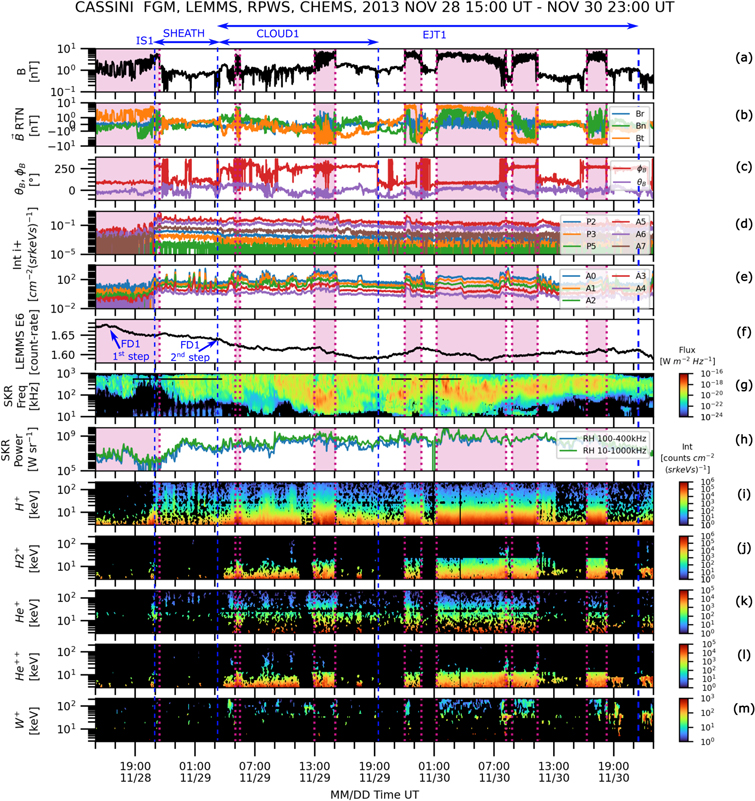
Figure 3. ICME1 signatures in magnetic field and plasma measurements, as seen by Cassini MAG/FGM, MIMI/LEMMS, RPWS, and MIMI/CHEMS. (a) Magnetic field strength. (b) Magnetic field components in RTN coordinates. (c) Magnetic field polar (θB ) and azimuthal (ϕB ) angles. (d) Energetic protons' intensity from LEMMS A5–A7 (0.6–4 MeV) and P2–P5 (2.3–11.4 MeV) channels. (e) Energetic protons' intensity from LEMMS A0–A4 (27–506 keV) channels. (f) GCR proton–dominated signal on LEMMS E6 count rate. The two steps of the FD associated with ICME1 (FD1) are marked with blue arrows. (g) SKR fluxes from RPWS. (h) SKR total emitted power. (i)–(m) Ion fluxes from CHEMS (3–220 keV). Purple shading indicates the spacecraft is in the magnetosheath and no shading is for the solar wind. Purple dotted lines mark BS crossings. Blue dashed lines mark ICME1 structures.
Download figure:
Standard image High-resolution image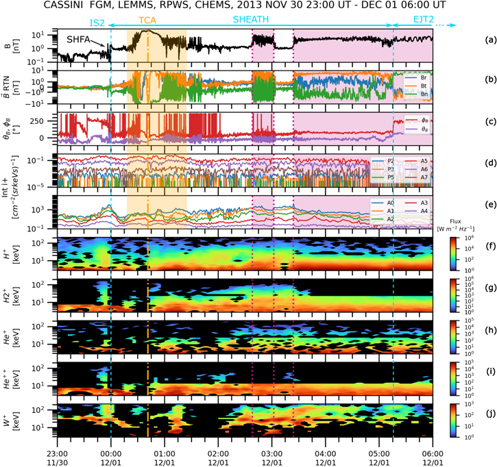
Figure 4. Zoomed-in view around the ICME2 interplanetary shock (IS2) and its sheath. Panels (a)–(e) are the same as those in Figure 3. Orange shading delimits Titan's magnetic signature. Spontaneous hot flow anomalies (SHFAs) are labeled with an arrow upstream from IS2 in (a). Panels (f)–(j) are the same as Figures 3(i)–(m). Cyan dashed lines mark ICME2 structures.
Download figure:
Standard image High-resolution image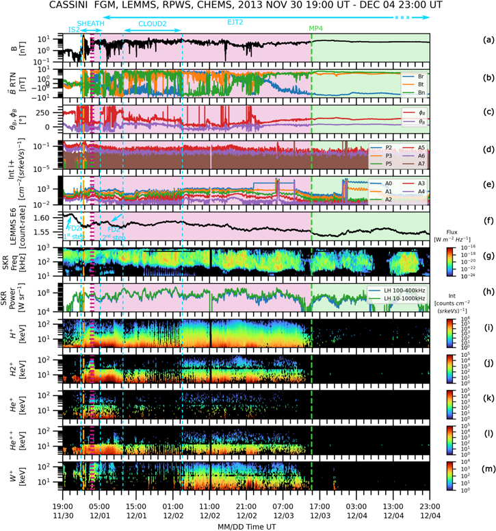
Figure 5. Same as Figure 3 but for ICME2 signatures. The two steps of the FD associated with ICME2 (FD2) are marked with cyan arrows in panel (f). The orange dashed–dotted line marks Cassini's closest approach to Titan (TCA). Cyan dashed lines mark ICME2 structures.
Download figure:
Standard image High-resolution imageTable 2. List of Saturn's BS Crossings from 2004 to 2016 Compressed beyond 20.2 RS (Titan's Mean Distance from Saturn)
| Year | DOY | Time | r0 (RS) | PSW (nPa) | SEP Events | Events of Solar Periodicity in GCRs |
|---|---|---|---|---|---|---|
| 2005 | 102 | 15:31 | 19.6 | 0.136 | 2-PERIODIC | |
| 2005 | 102 | 21:15 | 18.7 | 0.167 | ||
| 2005 | 102 | 22:07 | 18.5 | 0.173 | ||
| 2005 | 103 | 0:27 | 18.1 | 0.19 | ||
| 2005 | 103 | 1:09 | 18.0 | 0.196 | ||
| 2005 | 182 | 10:48 | 19.1 | 0.152 | ||
| 2005 | 182 | 15:23 | 19.7 | 0.133 | ||
| 2005 | 182 | 18:47 | 20.1 | 0.121 | ||
| 2007 | 33 | 23:50 | 17.0 | 0.252 | ||
| 2007 | 34 | 1:05 | 17.1 | 0.245 | ||
| 2007 | 34 | 2:50 | 17.2 | 0.237 | ||
| 2007 | 34 | 3:05 | 17.2 | 0.236 | ||
| 2007 | 71 | 6:10 | 20.1 | 0.12 | 5-PERIODIC | |
| 2007 | 71 | 15:05 | 19.9 | 0.125 | ||
| 2007 | 72 | 23:35 | 18.4 | 0.176 | ||
| 2007 | 73 | 1:35 | 18.3 | 0.182 | ||
| 2007 | 117 | 16:15 | 19.0 | 0.155 | ||
| 2007 | 117 | 23:25 | 19.0 | 0.155 | ||
| 2007 | 117 | 23:45 | 19.0 | 0.155 | ||
| 2007 | 164 | 21:25 | 19.5 | 0.137 | ||
| 2007 | 164 | 22:10 | 19.7 | 0.132 | ||
| 2007 | 164 | 23:30 | 20.0 | 0.124 | ||
| 2007 | 237 | 11:35 | 19.8 | 0.13 | 6-PERIODIC | |
| 2007 | 237 | 11:50 | 19.7 | 0.131 | ||
| 2007 | 237 | 11:55 | 19.7 | 0.132 | ||
| 2007 | 237 | 12:00 | 19.7 | 0.132 | ||
| 2007 | 237 | 12:25 | 19.6 | 0.135 | ||
| 2007 | 237 | 16:00 | 18.9 | 0.158 | ||
| 2008 | 99 | 0:24 | 20.0 | 0.124 | 18-SEP | 7-PERIODIC |
| 2008 | 99 | 4:13 | 19.5 | 0.139 | ||
| 2008 | 99 | 4:47 | 19.4 | 0.141 | ||
| 2008 | 192 | 13:07 | 20.0 | 0.125 | 8-PERIODIC | |
| 2008 | 192 | 14:30 | 20.0 | 0.124 | ||
| 2008 | 192 | 14:34 | 20.0 | 0.124 | ||
| 2008 | 192 | 15:05 | 20.0 | 0.124 | ||
| 2010 | 121 | 18:40 | 18.9 | 0.158 | 11-PERIODIC | |
| 2010 | 121 | 19:32 | 18.9 | 0.157 | ||
| 2010 | 122 | 0:40 | 19.1 | 0.149 | ||
| 2010 | 122 | 11:46 | 19.5 | 0.137 | ||
| 2010 | 122 | 14:30 | 19.6 | 0.134 | ||
| 2010 | 122 | 19:12 | 19.7 | 0.131 | ||
| 2010 | 122 | 23:42 | 19.8 | 0.128 | ||
| 2010 | 123 | 10:36 | 20.0 | 0.123 | ||
| 2010 | 123 | 11:11 | 20.0 | 0.123 | ||
| 2010 | 123 | 13:50 | 20.0 | 0.122 | ||
| 2010 | 123 | 15:45 | 20.1 | 0.122 | ||
| 2010 | 123 | 17:57 | 20.1 | 0.121 | ||
| 2010 | 124 | 3:02 | 20.1 | 0.12 | ||
| 2010 | 124 | 9:00 | 20.1 | 0.12 | ||
| 2010 | 124 | 11:38 | 20.1 | 0.121 | ||
| 2010 | 124 | 12:16 | 20.1 | 0.121 | ||
| 2010 | 124 | 18:45 | 20.1 | 0.121 | ||
| 2010 | 124 | 21:48 | 20.1 | 0.122 | ||
| 2010 | 125 | 2:29 | 20.0 | 0.123 | ||
| 2010 | 125 | 4:35 | 20.0 | 0.124 | ||
| 2010 | 194 | 1:55 | 20.0 | 0.124 | ||
| 2010 | 194 | 4:03 | 20.0 | 0.125 | ||
| 2010 | 194 | 8:40 | 19.9 | 0.128 | ||
| 2010 | 194 | 9:55 | 19.8 | 0.129 | ||
| 2011 | 21 | 18:25 | 19.4 | 0.141 | ||
| 2011 | 22 | 4:25 | 18.9 | 0.159 | ||
| 2011 | 22 | 5:39 | 18.8 | 0.162 | ||
| 2011 | 124 | 9:23 | 20.2 | 0.119 | ||
| 2011 | 306 | 22:51 | 19.2 | 0.148 | 22-SEP | |
| 2011 | 306 | 23:57 | 19.0 | 0.155 | ||
| 2011 | 307 | 1:34 | 18.7 | 0.166 | ||
| 2012 | 101 | 8:33 | 19.7 | 0.132 | 24-SEP | |
| 2012 | 206 | 22:49 | 19.4 | 0.14 | 26-SEP | |
| 2012 | 207 | 2:46 | 20.2 | 0.12 | ||
| 2013 | 157 | 23:41 | 17.4 | 0.226 | 29-SEP | 14-PERIODIC |
| 2013 | 334 | 16:20 | 20.0 | 0.123 | 31-SEP | |
| 2013 | 334 | 18:17 | 19.9 | 0.127 | ||
| 2013 | 335 | 2:37 | 19.2 | 0.148 | ||
| 2013 | 335 | 3:02 | 19.1 | 0.15 | ||
| 2013 | 335 | 3:23 | 19.1 | 0.151 | ||
| 2014 | 273 | 13:01 | 18.1 | 0.189 | 35-SEP | 15-PERIODIC |
| 2014 | 273 | 18:16 | 18.6 | 0.17 | ||
| 2014 | 359 | 21:12 | 19.9 | 0.125 | 37-SEP | |
Notes. The standoff distance r0 and associated solar wind dynamic pressure PSW are obtained with the Masters et al. (2008) model. Groupings with a value in the SEP Events column (a number with "-SEP") correlate with the event in Tables 1–3 of Roussos et al. (2018) indicated by the number, and groupings with a value in the final column (a number with "-PERIODIC") correlate with the event of the indicated number in Table 4 therein.
3.2.1. ICME1: Interplanetary Shock, Sheath, and Ejecta
ICME1 is identified with the crossing of an interplanetary shock (IS1) on November 28 at 20:57 UT (Roussos et al. 2018), as shown in Figure 3. IS1 is observed inside Saturn's magnetosheath, as a large rotation in ϕB
and a jump in Bt
, plus a magnetic field strength jump from ∼1.7 to ∼4.6 nT. In panel (f) the start of an FD can be noticed in the GCR proton count rate values on November 28 around 17:00 UT (FD1 1st step), which can be associated with the transit of IS1 (Richardson & Cane 2011). IS1 also stands out in the LEMMS A0–A7 and P2–P5 channels (panels (d) and (e)), as SEPs are accelerated at the shock front (Roussos et al. 2018) and fluxes peak on November 28 at 21:15 UT. The presence of energetic protons is also seen in the CHEMS H+ spectrogram (panel (i)), which spans an energy range similar to that of LEMMS A0–A4 and where an increase in fluxes is seen from a few keV to a couple hundred. In panels (j)–(l), flux enhancements of  , He+, and He++ are also seen around IS1.
After IS1 the interplanetary magnetic field (IMF) strength takes values of ∼0.85 nT, which are much higher than the typical ∼0.1 nT expected at Saturn's heliocentric distance (e.g., Witasse et al. 2017). This may indicate the spacecraft is transiting the compressed plasma of IS1's sheath. SEP fluxes remain strong at all energy channels, and so do the fluxes of protons and solar wind He+ seen with CHEMS. In panels (g) and (h) an enhancement of SKR emissions can be seen starting on November 28 at 23:10 UT, with total emitted power values rising up to 108 W sr−1. This is above the average range of 106–107 W sr−1 (Lamy et al. 2008) and indicates an enhanced solar wind dynamic pressure, compatible with a compression generated by IS1.
On November 29 at 03:15 UT a significant rotation and an enhancement of the magnetic field mark the start of ICME1's ejecta (EJT1). This perturbation is closely timed with a small variation in the decreasing slope of the LEMMS E6 count rate (around 03:30 UT), which we mark as a possible second step of the FD (FD1 2nd step) in Figure 3(f). According to Richardson & Cane (2011), an FD second step can be associated with the transit of the ICME's ejecta. The IMF strength reaches values as high as 1.9 nT and only returns to more typical values of ∼0.5 nT around November 30 at 21:45 UT, where we mark the end of the structure. In panels (g) and (h) we see SKR enhancements persist up until this time as well. The total emitted power reaches values as high as 1010, accompanied by low-frequency extensions (LFEs) that reach down to 15 kHz (Roussos et al. 2018). In addition, SEP fluxes remain strong through EJT1 at all energy channels. In particular, A0–A4 (panel (e)) show further flux enhancements that do not extend to the MeV range and correlate with Cassini's incursions in Saturn's magnetosheath. This complements CHEMS observations (panels (l)–(m)), which show ions are heated primarily at lower energies during the Kronian sheath incursions. For the protons this effect seems to add up to the dispersed heating generated by the ICME at a wide energy range.
Panels (a)–(c) show that within EJT1, from where it begins up until November 29 at 19:20 UT, a cloudlike structure can be distinguished with a smooth rotation in ϕB , Bn pointing north (when in the solar wind) and Bt pointing east, and a magnetic field enhancement, intensified by two short incursions in the sheath.
3.2.2. ICME2: Interplanetary Shock, Sheath, and Ejecta
As seen in Figure 4, ICME2 is detected on December 1 at 00:00 UT with the crossing of a second interplanetary shock (IS2), first reported by Bertucci et al. (2015) as a "shock front" with unclear origin. As IS2 occurs inside Saturn's foreshock, SHFAs, which have developed from foreshock cavities, are observed upstream (Omidi et al. 2017). The passage of IS2 perturbs the solar wind significantly, with the IMF jumping from ∼0.4 nT upstream from the shock (November 30 22:20–23:55) to ∼1 nT downstream (from December 1 00:02 onward), and reaching maximum values of ∼2 nT. As seen in panels (a)–(c), the main transition occurs in the Bn component, with the field rotating southward. IS2 is also a source of SEP acceleration. In panel (e) we see a peak in the LEMMS A channels at the time of the shock. There is no clear onset, compared to the peak around IS1, because SEP fluxes remain high. However, the increase is noticeable, especially as we go to lower-energy channels, where the intensity of the peak is comparable to the one on November 28. In panels (g) and (i) we see that prior to IS2 an energy threshold is visible for H2+ and He++. Bertucci et al. (2015) associated this with a cutoff energy up to which these ions are picked up by the solar wind, and estimated a corresponding solar wind speed of ∼460 km s−1. A decrease in the pickup ions' cutoff energy can be seen after IS2, which translates to a solar wind speed of ∼300 km s−1 (Bertucci et al. 2015). This is compatible with the plasma compression and deceleration caused by the shock. On November 30 around 21:30 UT, LEMMS E6 count rate values show a second significant drop, as seen in Figure 5(f). We mark this as the first step of an FD associated with ICME2 (FD2 1st step), which can be linked to the transit of IS2.
Through IS2's sheath, the IMF strength reaches values above 1 nT. This enhancement remains after Cassini's encounter with Titan (shaded in orange in Figure 4) and the Kronian BS crossings on December 1. The LEMMS P2 and A channels still show strong SEP fluxes (panels (d) and (e)), while CHEMS shows strong ion fluxes for all species, including the water-group ions W+ (panels (f)–(j)), probably due to the closer proximity of the spacecraft to Saturn and Titan.
On December 1 at 05:18 UT we mark the start of ICME2's ejecta (EJT2) based on the observation of a rotation in the magnetic field and a perturbation in the total field strength (Figures 4 and 5(a)–(c)). This is closely timed with a perturbation on LEMMS E6 count rate values, seen in Figure 5(f) around 07:00 UT, which we mark as a possible second step of the second FD (FD2 2nd step), though it is ambiguous if this is a random fluctuation of the data. Between December 1 at 11:40 UT and December 2 at 03:43 UT we observe a smoother magnetic field rotation region and further field enhancement that can be identified as a magnetic cloud, with Bt pointing west and Bn pointing north (Figures 5(a)–(c)). Around the start of the cloud, the signals of the LEMMS P channels drop, but fluxes remain significant in the A channels (Figures 5(d) and (e)). Note that the sharp, large increases and very-high-frequency oscillations observed at lower energies in A0–A4 are associated with spacecraft rotations.
Throughout EJT2, ion fluxes remain enhanced at a wide energy range when Cassini is in Saturn's magnetosheath, and drop suddenly at MP4, with the spacecraft entering the planet's magnetosphere (Figures 5(i)–(m)). In addition, SKR emissions remain enhanced up until December 4 at 19:53 UT. The total emitted power goes up to 109 W sr−1 and LFE episodes are observed, reaching frequencies around 20 kHz. The discontinuities observed in the SKR can be associated with the spacecraft entering the dusk region, where SKR emissions display lower intensities and limited viewing is expected (Lamy et al. 2008). Though fewer indicators remain, EJT2 may extend far past the magnetospheric boundary, as GCR count rate values continue to go down at least until December 9 (beyond the plotted interval of Figure 5).
The observation of ICME1 and ICME2 at 9.58 au is compatible with the expected arrival of multiple solar events that occur during early November. Around this time, Saturn is located between the two Solar Terrestrial Relations Observatory spacecraft (STEREO-A and STEREO-B) that orbit the Sun at ∼1 au (Kaiser et al. 2008). A selection of Saturnward events sufficiently strong to reach the outer solar system and drive interplanetary shocks yields three most probable candidates. These are (1) an ICME detected in situ by STEREO-A on 2013 November 4, at 08:56 UT, which is directly linked to a CME eruption on November 2 at 04:48 UT, with a speed of 1078 km s−1 as reported in the NASA Space Weather Database of Notifications, Knowledge, Information (DONKI) catalog 9 ; (2) an ICME seen by STEREO-B on November 6 at 02:00 UT, which has not yet been linked to a specific solar event; and (3) an ICME observed by STEREO-B on November 8 at 13:38 UT, directly linked to a CME eruption on November 7 at 10:39 UT, with a speed of 2100 km s−1 (DONKI). Using the Rouillard et al. (2017) radial propagation model, with STEREO observations as inputs, the expected arrival times at Saturn are December 3 at 00:36 UT for candidate (1), November 30 at 07:55 UT for candidate (2), and November 28 at 12:23 UT for (3). We presume that event (3), which is the strongest on the list, might be the one identified as ICME1 in Cassini's data, while either candidate (2) or a merger of (1) and (2) could have resulted in the signatures identified as ICME2.
3.3. Titan's Plasma Interaction with an ICME
Cassini encounters Titan's induced magnetosphere shortly after the detection of interplanetary shock IS2 (December 1 at 00:00 UT) during the T96 flyby. Titan's magnetic signature (BS and induced magnetosphere) starts from approximately December 1 at 00:24 (Bertucci et al. 2015) and is followed by a series of compressive structures until 01:42 UT.
In order to analyze the magnetic field and plasma that Titan interacts with, two intervals are considered to estimate the background IMF: 00:01:29–00:19:24 UT (along the flyby's inbound leg) and 01:43:17–01:58:34 UT (along the outbound leg). The average magnetic field yields (0.300, 0.127, −0.824) nT and (0.999, 0.184, −0.721) nT for the inbound and outbound intervals, respectively. The background field is the average of these two values: (0.650, 0.155, −0.773) nT. These values are given in TSWIS coordinates.
The Titan-centered draping (DRAP) coordinates are very useful for describing the pileup and draping typical of induced magnetospheres (Neubauer et al. 2006), and are defined from TSWIS as follows: the XDRAP axis is parallel to the XTSWIS axis and the solar wind flow, whereas the ZDRAP axis is antiparallel to the component of the background magnetic field perpendicular to the solar wind flow, that is, (0, 0.155, −0.773) nT. One way to assess the degree of agreement between the expected draping morphology and the Cassini MAG observations is to look for sign inversions of the magnetic field vector and spacecraft position vector components in DRAP coordinates.
Figure 6 shows 1 s resolution MAG/FGM data in DRAP coordinates along the spacecraft trajectory during T96. Panel (a) shows the magnetic field strength and (c) shows the Bz,DRAP component, on the ZDRAP–XDRAP plane. From these two views we conclude that (1) Cassini explores Titan's dayside magnetosphere for most of the T96 encounter (it crosses the XDRAP = 0 plane around 01:38:24 UT, at approximately ZDRAP = −7.6 RT); (2) the magnetic field component parallel to the background field increases with decreasing distance from Titan; and (3) Cassini's closest approach occurs inside Titan's lower MPR probably just above Titan's collisional ionosphere, where the magnetic field strength is expected to be low. All these signatures are compatible with a magnetic field pileup near the XDRAP axis, as seen in panel (e), where the Neubauer et al. (2006) draping sketch is illustrated.
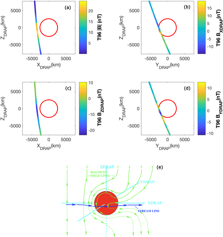
Figure 6. Magnetic field data from Cassini MAG/FGM in DRAP coordinates along the spacecraft trajectory during the T96 flyby. (a) Magnetic field strength in the Z–X plane. (b) Bx,DRAP component in the Z–Y plane. (c) Bz,DRAP component in the Z–X plane. (d) By,DRAP component in the Z–Y plane. The disk represents Titan's surface. (e) Sketch of the expected draping of frozen-in magnetic field lines near Titan according to Neubauer et al. (2006).
Download figure:
Standard image High-resolution imageFigure 6(b) shows the Bx,DRAP component on the ZDRAP–YDRAP plane. The dayside draping scheme described in Neubauer et al. (2006) requires a change in sign in Bx,DRAP at ZDRAP = 0. Accordingly, Cassini crosses the ZDRAP = 0 plane around 00:37:12 UT, just 1 minute before the change in sign from negative to positive (at 00:38:24 UT). Finally, panel (d) shows the By,DRAP magnetic field component on the ZDRAP–YDRAP plane, where a bipolar signature is observed. Although the By,DRAP > 0 signature in the third quadrant is compatible with the By,DRAP bulges described in Neubauer et al. (2006), the first By,DRAP > 0 signature around ZDRAP > 0 is not. With most of the encounter occurring on the YDRAP < 0 sector of Titan's induced magnetosphere, Cassini crosses the YDRAP = 0 plane around 00:55:48 UT.
The high degree of compatibility between the observations and the expected draping morphology from Neubauer et al. (2006) translates into an accurate determination of the background IMF that develops into Titan's induced magnetosphere—that is, the ambient field after the impact of IS2.
This is further supported by Figure 7, which shows the magnetic field data and the IMF clock angle  from the BS crossing seen on November 30 at 18:17 UT (event 19 in Table 1) up to Titan's encounter. In Figure 7(e), the horizontal band around −70° is the average clock angle measured in Titan's dayside MPR (± its standard deviation). Similar values are observed downstream from the interplanetary shock, and earlier the IMF clock angle is generally different from that measured inside Titan's magnetosphere. This supports the idea that the magnetic flux tubes hanging in Titan's induced magnetosphere during T96 belong to the ICME's structure (the IS2 sheath to be specific), rather than to the pristine solar wind.
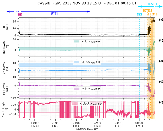
Figure 7. Compatibility between the piled-up magnetic field in Titan's dayside induced magnetosphere and the upstream IMF. (a) Magnetic field strength. (b)–(d) Magnetic field components in TSWIS. (e) Magnetic field clock angle. Shaded horizontal bands indicate the average of the corresponding parameter within the dayside MPR. Titan's magnetic signature is shaded in orange with the MPR in darker shading.
Download figure:
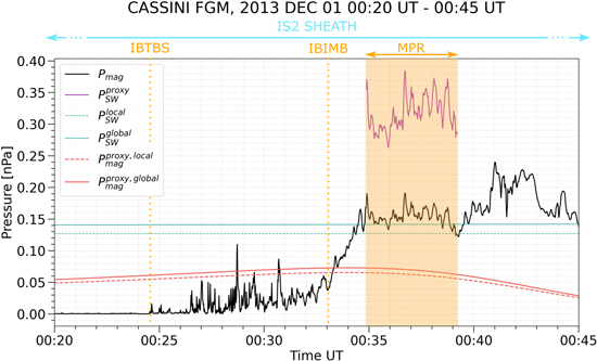
Standard image High-resolution imageA similar analysis can be drawn from the accumulated magnetic pressure in Titan's dayside induced magnetosphere. Figure 8 shows the in situ magnetic pressure around Titan's magnetic barrier, Pmag, and the resulting solar wind dynamic pressure proxy at the MPR, PSW
proxy, from the balance equation (1). It also shows the estimated solar wind dynamic pressures from M08, PSW
local and PSW
global (see Sections 2 and 3.1), and their derived magnetic pressure proxies,  and
and  , from Equation (1).
Figure 8. Magnetic and solar wind dynamic pressure around Titan's dayside magnetic barrier. Pmag is the in situ magnetic pressure obtained as B2/2μ0; PSW
proxy is the dynamic pressure obtained from the balance of the magnetic pressure at the MPR; PSW
local is the dynamic pressure estimated locally at the last BS crossing before Titan's encounter using the M08 model; PSW
global is similar to PSW
local but extrapolating the results from M08 for the plasma after the observed BS crossing; and  and
and  are the magnetic pressure proxies obtained from the balance of PSW
local and PSW
global, respectively.
are the magnetic pressure proxies obtained from the balance of PSW
local and PSW
global, respectively.
Download figure:
Standard image High-resolution image
As Cassini heads for Saturn,  (see Section 3.1) and the same applies for their respective magnetic pressure proxies. At the approximate location of Titan's inbound IMB (IBIMB), the proxies equal Pmag. However, at this point, the sharp gradient at the IBIMB means the in situ magnetic pressure abruptly surpasses the proxies, while these reach a maximum value and start to drop (modulated by
  ). At the MPR, Pmag reaches ∼0.15 nPa, doubling the maximum
  and
and  . This suggests that the magnetic pressure proxies underestimate the magnetic pressure accumulated in Titan's dayside magnetosphere. But also, the plot shows that the actual magnetic barrier at Titan occurs at a lower altitude than these magnetic pressure proxies' maxima predict.
If pressure balance is assumed, this means that Titan is exposed to an upstream dynamic pressure stronger than PSW local and PSW global. In fact, from PSW proxy, we find the solar wind dynamic pressure must be a factor 2 higher, around 0.32 nPa. This is in agreement with the dynamic pressure estimated with the P15 model around MP4, for which A06 predicts a pressure value more similar to PSW local and PSW global (see Section 3.1).
In any case, the results in Figures 7 and 8 indicate that Titan accumulates an extraordinary amount of magnetic flux along the direction of a background field compatible with the ambient conditions of IS2's sheath, and as a response to an equally strong upstream dynamic pressure impossible in the pristine solar wind.
4. Summary and Discussion
We analyzed Cassini field and particle data from 2013 late November to early December to study the plasma context around the T96 flyby, where Titan was found exposed to the solar wind on December 1 (Bertucci et al. 2015). By using statistical empirical models for Saturn's MP and BS (Arridge et al. 2006; Masters et al. 2008; Kanani et al. 2010; Pilkington et al. 2015), we studied the dynamics of Saturn's magnetosphere and found it was subjected to an unprecedented compression that lasted for 5+ days, from late November 28 to December 4 (at least). The MP and BS standoff distances reached values of ∼13–15 RS and 19 RS, respectively, under solar wind dynamic pressures of 0.16–0.3 nPa (depending on the model). These values are 7–14 RS less than the average location of the MP subsolar point (Achilleos et al. 2008), and 6 RS less than the average for the BS (Masters et al. 2008).
We found that the source of this magnetospheric compression was the sequential impact of two ICMEs on the Saturn–Titan system: the first one (ICME1) was seen between November 28 at 20:57 UT and November 30 at 21:45 UT, and the second one (ICME2) between December 1 at 00:00 UT and beyond December 4. Both ICMEs were first identified with the impact of an associated interplanetary shock (Bertucci et al. 2015; Roussos et al. 2018). The ICMEs' magnetic structures were delimited despite the spacecraft diving into and out of the solar wind and into Saturn's magnetosphere. This was achieved by analyzing a combination of direct and indirect ICME signatures. The former included the observation of magnetic field enhancements, with the IMF reaching up to ∼2 nT (well above the typical values at Saturn's heliocentric distance, e.g., Witasse et al. 2017), as well as periods of smoother magnetic field rotations compatible with flux-rope-type structures. Indirect proxies included the observation of two-stepped FDs, which indicate the passage of the interplanetary shock and the ICME magnetic obstacle (Richardson & Cane 2011); enhancements and LFEs of SKR emissions (Roussos et al. 2018; Cecconi et al. 2022); and enhanced ion fluxes.
As there was no indication of any transient disturbances in the plasma around Saturn–Titan before the encounter of the first interplanetary shock, we assumed that its sheath was the first source of magnetospheric compression and increased solar wind dynamic pressure, boosted by the subsequent passing of ICME1's body. After a short 2.25 hr period of quiet time conditions, not enough for Saturn's magnetosphere to "bounce back," the second interplanetary shock hit. Upstream conditions remained fueled by both the shocked plasma in the sheath and the following ICME2's ejecta.
We traced back the ICME transients observed by Cassini to their potential solar sources. We associated ICME1 with a strong CME eruption on November 7, and ICME2 with either an ICME seen at STEREO-B on November 6 (for which no clear CME event was provided), or a potential merger between this event and an ICME linked to an eruption on November 2. Further conclusions should require a dedicated study that includes simulations on the propagation of each event through the heliosphere using models such as the WSA-ENLIL cone model (Odstrcil 2003) or EUHFORIA (Pomoell & Poedts 2018). Cassini's observations with intermittent incursions in the solar wind, the lack of velocity measurements with which to study the helicity of the structures, and the fact that no spacecraft other than STEREO and Cassini recorded these ICMEs in situ make it a complex task to compare the observed magnetic structures or foresee potential interactions between the selected events.
The magnetic memory of the field piled up on Titan's dayside induced magnetosphere, which can fossilize plasma for up to ∼3 hr (Bertucci et al. 2008), pictured the solar wind that was present just a couple of minutes before Cassini's closest approach. This allowed us to reconstruct the background plasma environment that correlated to the magnetic signature Cassini observed at Titan. From analyzing the magnetic draping morphology (Neubauer et al. 2006) and the magnetic field orientation by means of the IMF clock angle, it turned out that the background field Titan interacted with was compatible with the ambient conditions within the second ICME structure (ICME2). More precisely, Titan was seen interacting with the plasma sheath from the second interplanetary shock. Comparisons between different proxies for the magnetic and dynamic pressure balance at the MPR (Spreiter & Stahara 1992) further support the hypothesis that Titan interacted with a perturbed solar wind.
Regarding the effects this interaction had on Titan's ionization conditions, T96 had a peak electron density of 103 cm−3 at ∼1400 km, which is higher than the average at that altitude and among the top values over the entire mission, but not uncommon during solar maximum. Above ∼1500 km, the density profile dropped rapidly, possibly due to the effect of the increased solar wind dynamic pressure. During the outbound leg of the flyby, a density peak of 200 cm−3 was seen at ∼1700 km, which could potentially be related to increased ionization from SEPs. However, as Cassini did not dive into lower altitudes during T96, a proper study of SEPs' contribution to these density enhancements should require particle simulations and further comparison with other flybys. In addition, based on observations at Mars and Venus (e.g., Edberg et al. 2010, 2011; Jakosky et al. 2015), we expect that higher doses of solar wind energy will also cause a significant increase in the atmospheric escape rate at Titan. This motivates yet another line of work, which would call for the modeling of Titan's magnetic tail under the observed upstream conditions.
Given the high degree of compression of Saturn's magnetosphere needed for Titan to be in the supersonic solar wind, the most likely scenario is for this to happen under strong space weather conditions. We took a list of 1349 BS crossings over the Cassini mission (2004–2016) (Cheng et al. 2022) and calculated their standoff distance and associated solar wind dynamic pressure using the M08 model. We found 78 of these BS crossings were compressed beyond 20.2 RS under pressures greater than 0.12 nPa, which could potentially expose Titan to the solar wind at some point of its orbit. As shown in Table 2, 61 of these crossings were successfully correlated with an event from the Roussos et al. (2018) catalog of SEPs (listed in Tables 1–3 therein, and referred to here with the tag "-SEP") or quasiperiodic GCR transients (listed in Table 4 therein, and referred to here with the tag "-PERIODIC").
Based on Roussos et al. (2018), some of these events could potentially be associated with an ICME and some with a corotating interaction region (CIR). Apart from event 31-SEP, which we associated with ICME1 and ICME2, the events that could be linked to an ICME are 22-SEP, 24-SEP, 26-SEP, 29-SEP, and 37-SEP, together with 14-PERIODIC, which is concurrent with 29-SEP. These occurred between 2011 October and 2014, during the rising phase and solar maximum of cycle 24, and were mostly strong to moderate intensity SEP events that lasted for more than two weeks and showed evidence of an FD. Events 2-PERIODIC, 5-PERIODIC, 6-PERIODIC, 7-PERIODIC, 8-PERIODIC, 11-PERIODIC, and 15-PERIODIC showed solar periodicity and mostly occurred between 2005 and 2010 during the declining phase of solar cycle 23 (with the exception of 15-PERIODIC, which occurred in 2014). This is compatible with the modulations generated by CIRs. Events 7-PERIODIC and 15-PERIODIC concur with low-intensity SEP events 18-SEP and 35-SEP, respectively, potentially being accelerated at the shock fronts of strong CIRs (Bučík et al. 2011). The BS crossings correlated with these potential CIR events were observed within the declining phase of the GCR count rate oscillations, which corresponds to the compression intervals of the CIRs.
As there is no significant difference between the pressure and standoff distance values obtained for the compressed BS crossings listed in Table 2, potentially, both ICMEs and CIRs are capable of compressing Saturn's magnetosphere enough to expose Titan to the solar wind. Either way, Titan would most likely interact with transient solar structures rather than with the pristine solar wind and, oftentimes, could be exposed to precipitating energetic particles that could deposit their energy in the lower parts of the moon's ionosphere.
The authors wish to thank I. Cheng for his collaboration and a preview of his work. The authors acknowledge financial support from Agencia I+D+i (Argentina) through grant PICT 2020-01707. S.B. is a CONICET PhD fellow. B.S.-C. acknowledges support from a UK-STFC Ernest Rutherford Fellowship ST/V004115/1. N.A. is supported by UK-STFC Consolidated Grant ST/S000240/1 (UCL-MSSL, University College London-Mullard Space Science Laboratory, Solar System). All Cassini data sets are publicly available at the NASA Planetary Data System (https://pds-ppi.igpp.ucla.edu/search/?sc=Cassini&t=Saturn). Magnetometer data supporting this work are publicly available on the Imperial College London MAGDA server (https://magda.imperial.ac.uk/).
Software: MIDL for Cassini (http://cassini-mimi.jhuapl.edu/MIDL/), AMDA (http://amda.cdpp.eu/), Propagation Tool (http://propagationtool.cdpp.eu/) (Rouillard et al. 2017).