


Abstract
Microlensing events have historically been discovered throughout the Galactic bulge and plane by surveys designed solely for that purpose. We conduct the first multiyear search for microlensing events on the Zwicky Transient Facility (ZTF), an all-sky optical synoptic survey that observes the entire visible northern sky every few nights. We discover 60 high-quality microlensing events in the 3 yr of ZTF-I using the bulk lightcurves in the ZTF Public Data Release 5.19 of our events are found outside of the Galactic plane (∣b∣ ≥ 10°), nearly doubling the number of previously discovered events in the stellar halo from surveys pointed toward the Magellanic Clouds and the Andromeda galaxy. We also record 1558 ongoing candidate events as potential microlensing that can continue to be observed by ZTF-II for identification. The scalable and computationally efficient methods developed in this work can be applied to future synoptic surveys, such as the Vera C. Rubin Observatory's Legacy Survey of Space and Time and the Nancy Grace Roman Space Telescope, as they attempt to find microlensing events in even larger and deeper data sets.
Export citation and abstract BibTeX RIS
1. Introduction
Einstein (1936) first derived that objects with mass could bend the light of a luminous star on its way to an observer and produce multiple images of the background star. This phenomenon is called gravitational microlensing because the individual images are separated by microarcseconds and are therefore unresolvable to any instrument. The observer can only measure a lightcurve that includes both the constant luminosity of the lens and the apparent increase in the brightness of the background star (Refsdal & Bondi 1964). Microlensing events will last as long as there is an apparent alignment, occurring on timescales ranging from days to years for one star magnifying another within the Milky Way (Paczyński 1986).
The amplification of the luminous source is maximized at the time (t0) when the projected separation between the source and lens on the sky is minimized. The degree of amplification is set by the impact parameter (u0), which is the minimum separation divided by the characteristic interaction cross section or Einstein radius,

where πrel = πL − πS which is the difference in parallax between the lens and source. The duration of this amplification, named the Einstein crossing time (tE), is the time over which θE is traversed by the relative proper motion between the lens and source (μrel),

For more thorough definitions of these parameters we refer the reader to Gould (1992).
Microlensing can be distinguished from other astrophysical transients due to several unique characteristics. The amplification of a source is ideally followed by a decrease in the source's brightness that is symmetric across the point of maximum amplification when a constant velocity for the lens and source is assumed. However, this symmetry is complicated by the nonuniform motion of Earth as it orbits around the Sun (Gould 1992), which produces a quasi-annual variation to the source amplification known as the microlensing parallax (πE ),

Either the symmetry of the observable lightcurve when there is low parallax or the presence of an annual variation to the amplification where there is high parallax is evidence of microlensing.
The amplification of the background star is achromatic as the geometric effects of bending spacetime occur equally for all wavelengths of light. However, the constant presence of the lens light in the lightcurve will produce a chromatic effect called blending (Di Stefano & Esin 1995). Imagine a source star that only emits flux at a red wavelength and a lens star of equal flux that only emits at a blue wavelength. Before (and after) the microlensing event, the brightness measured in corresponding red and blue filters could be equal to each other, but during the event the red filter would increase in brightness while the blue filter measured a constant flux, leading to a chromatic effect. This is further complicated by the presence of multiple neighbor stars not close enough to be involved in the microlensing phenomenon but within the point-spread function (PSF) of the instrument. These stars contaminate the lightcurve and also contribute additional unamplified light that causes chromatic blending. Together these effects produce a chromatic signal that can be modeled as a combination of unamplified and amplified light. The fraction of light that originates from the source (as compared to the light from the unamplified lens and neighbors) is given the name source-flux fraction or bsff.
The probability of two stars crossing the same line of sight is proportional to the apparent stellar density. This has motivated most microlensing surveys to look for events toward the Galactic bulge (Sumi et al. 2013; Udalski et al. 2015; Navarro et al. 2017; Kim et al. 2018; Mróz et al. 2019), as well as the Magellanic Clouds (Alcock et al. 2000; Tisserand et al. 2007; Wyrzykowski et al. 2011a, 2011b) and M31 (Novati et al. 2014; Niikura et al. 2019). These surveys discover hundreds to thousands of microlensing events per year. There have been fewer microlensing surveys dedicated to looking for these events throughout the Galactic plane. The Expérience pour la Recherche d'Objets Sombres (EROS) spiral arm surveys (Rahal et al. 2009) observed 12.9 million stars across four directions in the Galactic plane and discovered 27 microlensing events over 7 yr between 1996 and 2002. The Optical Gravitational Lensing Experiment (OGLE; Mróz et al. 2020b) discovered 630 events in 3000 deg2 of Galactic plane fields in the 7 yr between 2013 and 2019. They measured a threefold increase in the average Einstein crossing time for Galactic plane events as compared to the Galactic bulge and an asymmetric optical depth that they interpret as evidence of the Galactic warp. Mróz et al. (2020a) found 30 microlensing candidates in the first year of Zwicky Transient Facility (ZTF) operations.
While the number of events discovered thus far is much smaller than in Galactic bulge fields, simulations predict that there are many more events left to discover in large synoptic surveys. Sajadian & Poleski (2019) predict that the Vera Rubin Observatory Legacy Survey of Space and Time (LSST) could discover anywhere between 7900 and 34,000 microlensing events over 10 yr of operation depending on its observing strategy. Medford et al. (2020) estimate that ZTF would discover ∼1100 detectable Galactic plane microlensing events in its first 3 yr of operation, with ∼500 of these events occurring outside of the Galactic bulge (ℓ ≥ 10°). Microlensing events throughout the Galactic plane can yield interesting information about Galactic structure and stellar evolution that we cannot learn from only looking toward the Galactic bulge.
Gravitational lenses only need mass but not luminosity in order to create a microlensing event, thereby making microlensing the only method available for detecting a particularly interesting nonluminous lens object: isolated black holes. Inspired by the suggestion of Paczyński (1986) that places constraints on the amount of dark matter found in MAssive Halo Compact Objects (MACHOs) that could be measured by microlensing, there had been ongoing efforts to find these MACHOs, including black holes, as gravitational lenses for many years. The MACHO (Alcock et al. 2000) and EROS (Afonso et al. 2003) projects calculated these upper limits after several years of observations toward the Galactic bulge and Magellanic Clouds. While black hole candidates have been proposed from individual microlensing lightcurves (Bennett et al. 2002; Wyrzykowski et al. 2016), there is a degeneracy between the mass of the lens and the distances to the source and lens that cannot be broken through photometry alone. Essentially, photometry cannot distinguish between a massive lens that is relatively distant and a less massive lens that is closer to the observer. Lu et al. (2016) outlined how direct measurement of the apparent shift in the centroid of the unresolved source and lens, or astrometric microlensing, can be used to break this degeneracy and confirm black hole microlensing candidates. This shift is extremely small, on the order of milliarcseconds, and therefore requires high-resolution measurements on an adaptive optics system such as Keck AO. Several candidates have been followed up using this technique (Lu et al. 2016) and one possible black hole has been detected (Lam et al. 2022; Sahu et al. 2022; Mróz et al. 2022). Only a few can be rigorously followed up astrometrically and the astrometric signal of events found toward the bulge is at the edge of current observational capabilities. Simulations indicate that black hole candidates can be ideally selected from a list of microlensing events by searching for those with larger Einstein crossing time and smaller microlensing parallaxes (Lam et al. 2020). Furthermore, simulations indicate that events in the Galactic plane have larger microlensing parallaxes and astrometric shifts overall that can make finding black hole candidates among these surveys easier than surveys pointed toward the Galactic bulge (Medford et al. 2020).
In this paper, we conduct a search for microlensing events in the ZTF data set that is optimized to find these black hole candidates, increasing the number of candidates that can be astrometrically followed up for lens mass confirmation. Though the approach is mildly optimized for long-duration events, the pipeline is equipped to find microlensing events with a range of durations. A previous version of this approach appeared in the thesis by Medford (2021a). In Section 2, we discuss the ZTF telescope, surveys, and data formats. In Section 3, we outline the software stack we have developed to ingest and process lightcurve data for microlensing detection. In Section 4, we outline the steps taken to construct the detection pipeline used to search for microlensing in ZTF's all-sky survey data. In Section 5, we analyze the results of our pipeline and share our list of microlensing candidates. We conclude with a discussion in Section 6. Note, an understanding of Sections 2.2.1 and 3 is not required to understand the methodology, results, and discussion presented in Sections 4–6.
2. ZTF
2.1. Surveys and Data Releases
ZTF began observing in 2018 March as an optical time-domain survey on the 48 inch Samuel Oschin Telescope at Palomar Observatory (Bellm et al. 2019b; Graham et al. 2019). In the almost 3 years of Phase-I operations, ZTF has produced one of the largest astrophysical catalogs in the world. Nightly surveys were carried out on a 47 deg2 camera in the ZTF g-band, r-band and i-band filters averaging ∼2 0 FWHM on a plate scale of 101 pixel−1. The surveys during this time were either public observations funded by the National Science Foundation's Mid-Scale Innovations Program, collaboration observations taken for partnership members and held in a proprietary period before later being released to the public, or programs granted by the Caltech Time Allocation Committee (Bellm et al. 2019a).
Three surveys of particular interest for microlensing science are the Northern Sky Survey and the Galactic Plane Survey, both public, and the partnership High-Cadence Plane Survey. The Northern Sky Survey observed all sky north of −31° decl. in the g band and r band with an inter-night cadence of 3 days, covering an average of 4325 deg2 per night. The Galactic Plane Survey (Prince & Zwicky Transient Facility Project Team 2018) observed all ZTF fields falling within the Galactic plane (−7° < b < 7°) in the g band and r band every night that the fields were visible, covering an average of 1475 deg2 per night. These two public surveys have been run continuously since 2018 March. The collaboration High-Cadence Plane Survey covered 95 deg2 of Galactic plane fields per night with 2.5 hr continuous observations in the r-band totaling approximately 2100 deg2. ZTF Phase-II began in December 2020 with a public 2 night cadence survey of g-band and r-band observations of the northern sky dedicated to 50% of available observing time.
The resulting data from these surveys is reduced and served to the public by the Infrared Processing and Analysis Center (IPAC) in different channels tailored to different science cases (Masci et al. 2018). IPAC produces seasonal data releases (DRs) containing the results of the ZTF processing pipeline taken under the public observing time and a limited amount of partnership data. The products included in these data releases include instrumentally calibrated single-exposure science images, both PSF and aperture source catalogs from these individual exposures, reference images constructed from a high-quality set of exposures at each point in the visible sky, an objects table generated from creating source catalogs on these reference images, and lightcurves containing epoch photometry for all sources detected in the ZTF footprint. There have been DRs released every 3–6 months, starting with DR1 on 2019 May 8. As discussed in more detail in Section 3.2, this work exclusively uses data publicly available in DR3, DR4, and DR5 released on 2021 March 31. 3
These observations cover a wide range of Galactic structure in multiple filters with almost daily coverage over multiple seasons. ZTF's capability of executing a wide-fast-deep-cadence opens an opportunity to observe microlensing events throughout the Galactic plane that microlensing surveys only focused in the Galactic bulge cannot observe with equivalent temporal coverage. Our previous work simulating microlensing events observable by ZTF (Medford et al. 2020) indicated that there exists a large population of microlensing events both within and outside of the Galactic bulge yet to be discovered. We seek to find black hole microlensing candidates among these events that could be later confirmed using astrometric follow-up.
2.2. Object Lightcurves
While the real-time alert stream is optimized for events with timescales of days to weeks, black hole microlensing events occur over months or even years. Fitting for microlensing events requires data from both a photometric baseline outside of the transient event and the period during which magnification occurs (t0 ± 2tE). The data product therefore most relevant to our search for long-duration microlensing events are the data release lightcurves containing photometric observations for all visible objects within the ZTF footprint.
Data release lightcurves are seeded from the PSF source catalogs measured from co-added reference images. PSF photometry measurements from each single-epoch image are appended to these seeds where they occur in individual epoch catalogs. A reference image can only be generated when at least 15 good-quality images are obtained, limiting the locations in the sky where lightcurves can be found to parts of the northern sky observed during good weather at sufficiently low airmass. This sets the limit on the declination at which the Galactic plane is visible in data release lightcurves and consequently our opportunity to find microlensing events in these areas of the sky. Statistics regarding the lightcurve coverage for nearly a billion objects have been collated from the DR5 overview into Table 1.
Table 1. Object Statistics for Public DR5
| Filter | Accessible Sky Coverage | Nlightcurves | Nlightcurves with Nobs ≥ 20 |
|---|---|---|---|
| g band | 97.66% | 1,226,245,416 | 582,677,216 |
| r band | 98.31% | 1,987,065,715 | 1,107,250,253 |
| i band | 51.88% | 346,398,848 | 78,425,164 |
Note. Additional details can be found at https://www.ztf.caltech.edu/page/dr5.
Download table as: ASCIITypeset image
Observation fields are tiled over the night sky in a primary grid, with a secondary grid slightly shifted to cover the chip gaps created by the primary grid. The lightcurves are written into separate lightcurve files, one for each field of the ZTF primary and secondary grids and spanning approximately 7° × 7° each. In each one of these lightcurve files is a large ASCII table with a single row detailing each lightcurve metadata (including R.A., decl., number of epochs, and so forth), followed by a series of rows containing the time (in heliocentric Modified Julian Date, or hMJD), magnitude, magnitude error, the linear color coefficient term from photometric calibration, and photometric quality flags for each single-epoch measurement. These lightcurve files are served for bulk download from the IPAC web server and total approximately 8.7 TB.
A detailed summary of the terminology used in the ZTF catalog follows in Section 2.2.1. Here, we provide a concise summary; see also Figure 1. We emphasize that lightcurve files and lightcurves are distinct. Stars each have a unique R.A. and decl. and are assumed to be individual astrophysical objects. These stars may be several astrophysical stars blended together. Each star is associated with multiple sources that have different fields and readout channels due to ZTF's observing patterns. These are stored in lightcurve files, which are ASCII files with many lightcurves that all share the same field. If a star is associated with multiple sources in the same field but with different readout channels, there will be multiple sources associated with the same star in one lightcurve file. Each source is associated with 1–3 objects with each object having a unique filter; we call all the objects associated with one source siblings. Finally, each object is associated with a unique lightcurve.

Figure 1. Diagram of how observational information is stored in the PUZLE pipeline. An object is a set of observations at the same sky position taken on the same field, readout channel, and filter. A source can contain multiple objects from the same field and readout channel that are each different filters. We refer to multiple objects associated with the same source as siblings. This distinction exists because observations in different filters are assigned different identification numbers in the ZTF public data releases. One star can have multiple sources across lightcurve files, so all sources are cross referenced with each other by sky location and together form a single star. A lightcurve file is an ASCII file containing all the lightcurves associated with the same field, so it contains lightcurves from many stars. If a star has multiple sources with the same field, but different readout channels due to a shift in position caused by pointing errors, then the star will have multiple sources in the same lightcurve file.
Download figure:
Standard image High-resolution image2.2.1. Catalog Terminology
Continuing to discuss the structure of the lightcurve files requires a consistent vocabulary for describing this data product, which we introduce here for clarity. A diagram of the terms introduced here is shown in Figure 1. An object refers to a collection of photometric measurements of a single star in a single filter, in either the primary or secondary grid (but not both). Objects are written in the lightcurve files, which are associated with a unique field, grouped by their readout channel into sources. A source refers to the total set of objects within a single lightcurve file that are all taken at the same sky location and are assumed to arise from the same astrophysical origin. There can be a maximum of three objects per source for the three ZTF filters. Crowding in dense Galactic fields will often result in different astrophysical signals falling in the same PSF and therefore the same object. We address this issue during our microlensing fitting. Each of the objects within a single source are siblings to one another and have mutually exclusive filters. Siblings must share the same readout channel within a lightcurve file. A star refers to all sources of the same astrophysical origin found in all of the lightcurve files, so the star will have multiple sources if it has been captured by both the primary and secondary grids or if the star appeared on multiple readout channels. While many of these measurements will not be stars but in fact several stars blended together, galaxies, or other astrophysical phenomena, we adopt this nomenclature to serve our purpose of searching for microlensing events mainly in the Galactic plane. Each star contains one or more sources, with each source containing one or more objects, with each object containing one lightcurve.
There are several limitations inherent to the construction of these lightcurves that we have addressed in our work. First, the lightcurves for each filter are created from independent extraction of each filter's single-epoch flux measurement at a given location of the sky. Flux measurements in the g-band, r-band, and i-band filters from a single astrophysical origin will have three separate object IDs at three different locations in the lightcurve file with no association information present relating the three objects to each other. In terms of our nomenclature, it is unknown whether a source will have one, two, or three objects until the entire lightcurve file is searched row by row.
Second, objects found in different fields in the ZTF observing grid are also not associated with each other despite coming from the same astrophysical origin. The ZTF secondary grid intentionally overlaps with the primary grid to increase coverage in the gaps between readout channels and fields found in the primary grid. However, this results in single filter measurements from the same star being split into two primary and secondary grid lightcurve files. We have found instances where telescope-pointing variations have resulted in the same star having sources located in two different primary grid lightcurve files or the same star being recorded in multiple readout channels leading to multiple sources in one lightcurve file. Therefore, it is unknown whether a single star will contain one or more sources without searching through both the primary and secondary grid lightcurve files, or searching adjacent lightcurve files for those stars that fall on the edges of each field.
Third, the format of the lightcurve files are raw ASCII tables. While this format is exchangeable across multiple platforms and therefore reasonably serves the purpose of a public data release, ASCII is suited to neither high-speed streaming of the data from disk to memory nor searching for objects with particular properties without reading through an entire file. If we are to search for microlensing events throughout the entire ZTF catalog, then we must either ingest these lightcurve files into a more traditional database structure or create a method for efficiently reading these lightcurve files that provides the benefits of a database structure.
3. Software
We have developed a set of software tools to address the outstanding issues with the data release lightcurve data product. These tools are a mixture of public open-source codes and internal codes that enable efficient access to the data contained in the lightcurve files despite their ASCII format. The functionality and availability of these tools proved essential to scaling out microlensing search methods to the entire ZTF lightcurve catalog. However, these tools and approaches would prove generally useful to any science that seeks to execute a large search across the entire set of bulk lightcurves. We will therefore outline our approach in a level of technical detail that would aid another researcher attempting to similarly carry out such a large-scale search using the publicly available ZTF lightcurves.
3.1. zort: ZTF Object Reader Tool
A reasonable initial approach to reading the lightcurve files would be to ingest all of the data into a relational database where objects could be cross referenced against each other to construct sources and sources cross referenced against each other to construct stars. Flux measurements could be organized by object ID and an association table created to match these measurements to the metadata for each object. However, this approach has two major drawbacks. For science cases where the lightcurve files are used not as a search catalog but instead as an historical reference for a singular object of interest, it is overkill to ingest all data into an almost 8 TB database. Additionally, our approach aims to leverage the computational resources available at the NERSC Supercomputer located at the Lawrence Berkeley National Laboratory. Here, we can simultaneously search and analyze data from different locations in the sky by splitting our work into parallel processes. We would experience either race conditions or the need to exclusively lock the table for each process' write if all of our processes were attempting to read and write to a singular database table. Relational database access is a shared resource at NERSC, compounding this problem by putting a strict upper limit on the number of simultaneous connections allotted to single users when connecting to a database on the compute platform. These bottlenecks would negate the benefits of executing our search on a massive parallel supercomputer. We therefore sought a different method for accessing our data that would keep the data on disk and allow for so-called embarrassingly parallel data access.
The ZTF Object Reader Tool, or zort, is an open-source Python package that serves as an access platform into the lightcurve files that avoids these bottlenecks (Medford 2021b). It is a central organizing principle of zort that keeping track of the file position of an object makes it efficient to locate the metadata and lightcurve of that object. To enact this principle, zort requires four additional utility products for each lightcurve file. These products are generated once by the user to initialize their copy of a data release by running the zort-initialize executable in serial or parallel using the Python mpi4py package.
During initialization, each line of a lightcurve file (extension .txt) containing the metadata of an object is extracted and placed into an objects file (extension .objects), with the file position of the object within the lightcurve file appended as an additional piece of metadata. This file serves as an efficient way to blindly loop through all of the objects of a lightcurve file. For each object in the objects file, zort will jump to the object's saved file position and load all lightcurve data into memory when requested. Additionally, a hash table with the key-value pair of each object's object ID and file position is saved to disk as an objects map (extension .objects_map). This enables near-immediate access to any object's metadata and lightcurve simply by providing zort with an object ID.
Next, a k-d tree is constructed from the sky positions for all of the objects in each readout channel and filter within a lightcurve file and consolidated into a single file (extension .radec_map). This k-d tree enables the ability to quickly locate an object with only sky position. Lastly, a record of the initial and final file position of each filter and readout channel within a lightcurve file is saved (extension .rcid_map). Lightcurve files are organized by continuous regions of objects that share a common filter and readout channel, and by saving this readout channel map we are able to limit searches for objects to a limited set of readout channels if needed.
zort presents the user with a set of Python classes that enable additional useful features. Lightcurve files are opened with the LightcurveFile class that supports opening in a with context executing an iterator construct for efficiently looping over an objects file by only loading objects into memory as needed. This with context manager supports parallelized access with exclusive sets of objects sent to each process rank, as well as limiting loops to only specific readout channels using the readout channel map. Objects loaded with the Object class contain an instance of the Lightcurve class. This Lightcurve class applies quality cuts to individual epoch measurements as well as color correction coefficients if supplied with an object's PanSTARRS g-minus-r color. Objects contain a plot_lightcurves method for plotting lightcurve data for an object alongside the lightcurves of its siblings. Each object has a locate_siblings method that uses the lightcurve file's k-d tree to locate coincident objects of a different filter contained within the same field. The package has a Source class for keeping together all sibling objects of the same astrophysical origin from a lightcurve file. Sources can be instantiated with either a list of object IDs or by using the utility products to locate all of the objects located at a common sky position. zort solves all problems related to organizing and searching for objects across the R.A. polar transition from 360° to 0° by projecting instrumental CCD and readout channel physical boundaries into spherical observation space and transforming coordinates.
zort has been adopted by the ZTF collaboration and TESS-ZTF project as a featured tool for extracting and parsing lightcurve files. zort is available for public download as a GitHub repository (https://github.com/michaelmedford/zort) and as a pip-installable PyPi package (https://pypi.org/project/zort/).
3.2. PUZLE: Pipeline Utility for ZTF Lensing Events
Our search for microlensing events sought to combine all flux information from a single astrophysical origin by consolidating all sources into a single star. This required a massive computational effort as flux information was scattered across different lightcurve files as different objects with independent object IDs. First, we identified all sources within each lightcurve file by finding all of the siblings for each object within that file. Then sources in different lightcurve files at spatial coincident parts of the sky were cross referenced with each other to consolidate them into stars. To execute this method, as well as apply microlensing search filters and visually examine the results of this pipeline via a web interface, we constructed the Python Pipeline Utility for ZTF Lensing Events or PUZLE. Similar to the motivations for constructing zort, this package needed to take advantage of the benefits of massive supercomputer parallelization without hitting the bottlenecks of reading and writing to a single database table.
The PUZLE pipeline began by dividing the sky into a grid of adaptively sized cells that contain an approximately equal number of stars. Grid cells started at δ = −30°, α = 0° and were drawn with a fixed height of Δδ = 1° and a variable width of 0 125 ≤ Δα ≤ 20 at increasing values of α. We attempted to contain no more than 50,000 objects within each cell using a density determined by dividing the number of objects present in the nearest located lightcurve file by the file's total area. The cells were drawn up to α = 360°, incremented by Δδ = 10, and repeated starting at α = 0°, until the entire sky had been filled with cells. The resulting grid of 38,819 cells can be seen in Figure 2. Each of these cells represents a mutually exclusive section of the sky that was split between parallel processes for the construction of sources and stars.

Figure 2. Processing jobs for the PUZLE pipeline (top) and density of objects with a minimum number of observations (with catflag < 32768; bottom) throughout the sky, with the boundaries of the Galactic plane outlined in black. Job cells were sized to enclose approximately the same number of sources resulting in a larger number of smaller sized jobs in the areas of the sky with more objects per square degree. All job cells had a fixed height of 1° and a variable width between 0125 and 20. The limitations of a Galactic survey from the Northern hemisphere are also seen in the lack of sources near the Galactic Center.
Download figure:
Standard image High-resolution imageA PostgreSQL database was created to manage the execution of these parallel processes. This table was vastly smaller than a table that would contain all of the sources and stars within ZTF and was therefore not subject to the same limitations as previously stated for applying relational databases to our work. We created two identify tables, each containing a row for each cell in our search grid, one for identifying sources and one for identifying stars. Each row represented an independent identify_job that was assigned to a compute core for processing. Each row contained the bounds of the cell, and two Boolean columns for tracking whether a job had been started and/or finished by a compute core. Historical information about the date and unique compute process ID was also stored in the row for debugging purposes. To ensure that per-user database connection limits were not exceeded, we used an on-disk file lock. A parallel process had to be granted permission to this file lock before it attempted to connect to the database, thereby offloading the bottleneck from the database to the disk.
Here, we describe how each identify_job script worked, whether it is identifying sources or stars. An identify_job script was submitted to the NERSC supercomputer requesting multiple compute cores for a fixed duration of time. A script began by each compute core in the script fetching a job row from the appropriate identify table that was both unstarted and unfinished and marked the row as started. The script then identified all of the sources (or stars) within the job bounds as described below. The resulting list of sources (or stars) was then written to disk for later processing. Lastly, the job row in the identify table was marked as finished. Each script continued to fetch and run identify_jobs for all of its compute cores until just before the compute job was set to expire. At this time it interrupted whichever jobs were currently running and reset their job row to mark them as unstarted. In this way the identify table was always ready for any new identify_job script to be simultaneously run with any other script and ensure that only unstarted and unfinished jobs were run. The identify_job script for stars could only request jobs where the associated script for sources had finished.
The identify_job for finding sources began by finding the readout channels within all of the lightcurve files that intersected with the spatial bounds of its job by using the projected readout channel coordinates calculated by the zort package. Special attention was paid here to lightcurve files that cross the R.A. polar boundary between 360° and 0° to ensure that they were correctly included in jobs near these boundaries. Objects within the readout channels that overlap with the job were then looped over using the zort LightcurveFile class and those objects outside of the bounds of the job were skipped. Objects with fewer than 20 epochs of good-quality observations were also skipped over as this cut is an effective way to remove spurious lightcurves arising from erroneous or nonstationary seeds (see Figure 3 on the DR5 page). The remaining objects had their siblings located using the locate_siblings method and all of the siblings were grouped together into a single source. Once all of the lightcurve files had been searched, the remaining list of sources was cut down to only include unique sources with a unique set of object IDs. This prevented two duplicate sources from being counted, such as when a g-band object pairs with an r-band sibling, and that same r-band object pairs with that same g-band object as its sibling. Each source was assigned a unique source ID. The object IDs and file positions of all objects within each source were then written to disk as a source file named for that identify_job. In addition to this source file, a hash table similar to the zort objects_map file was created. This source map was a hash table with key-value pairs of the source ID and file position within the source file where that source was located.

Figure 3. Example ZTF objects and their η values, with individual epochs (blue) and nightly averages (red). DR5 lightcurves contained various cadences and gaps in the data depending on their visibility throughout the year and on which ZTF surveys were executed at their location. This resulted in a heterogeneous data set that required a flexible approach. The η statistic was able to capture inter-epoch correlation despite these different observing conditions, with smaller η signaling more correlated variability in the lightcurve. Note that the data plotted was cleaned using catflag < 32768.
Download figure:
Standard image High-resolution imageThe identify_job for finding stars began by loading all of the sources for that job directly from the on-disk file written by the source script. The sky coordinate of each source was loaded into a k-d tree. Each source's neighbors located within 2'' were found by searching through this tree. Sources were grouped together to form a star. A star's location was calculated as the average sky coordinate of its sources and the star defined as the unique combination of source IDs that it contains. Each star was assigned a unique ID. The star ID, sky location, and list of source IDs of each star were written to disk in a star file. A star map similar to the source map described above was also written to disk.
3.3. Upgrading to a New Public Data Release
Our approach of using the file position to keep track of objects and sources was able to transition between different versions of the public data releases when available. We used an older data release as a seed release upon which we initially searched for sources and stars. For this microlensing search and by way of example, we used DR3 as a seed release and updated our source and star files to DR5. We began by creating the necessary zort utility products for DR5 lightcurve files. We sought to append additional observations to our seed list of sources and stars. However, we did not look to find any additional objects that did not exist in DR3. The convention for different data releases is to keep the same object IDs for reference sources found at the same sky coordinates and to add new IDs for additional objects found. Therefore, when updating a row in the source file from DR3 to DR5 we only needed to use the source's object IDs and the DR5 object map to find the file location of the object in the DR5 lightcurve file. We found that in this process less than 0.02% of the object IDs in a source file could not be located in the DR5 object map and were dropped, resulting in a 99.98% conversion rate that was acceptable for our purposes. A new DR5 source map was then generated for this DR5 source file. Star files did not need to be updated and could be simply copied from an older to a newer data release. It should be noted that the names of lightcurve files slightly change between data releases, as the edge sky coordinates are printed into the file names and are a function of the outermost object found in each data release for that field. Any record keeping that involved the names of these lightcurve files needed to be adjusted accordingly.
4. Detection Pipeline
With our pipeline, we sought to measure the tE distribution for long-duration microlensing events (tE ≥ 30 days) in order to search for a statistical excess due to black hole microlensing. Second, we sought to generate a list of black hole candidates that could be followed up astrometrically in future studies. We therefore made design choices optimized for increasing the probability of detecting these types of events, even at the expense of short-duration events. We designed our pipeline to remove the many false positives that a large survey like ZTF can generate, even at the expense of false negatives. Our detection pipeline had to be capable of searching through an extremely large number of objects, sources, and stars and therefore had to be both efficient and computationally inexpensive to operate. These two priorities informed each of our decisions when constructing our microlensing detection pipeline. In our pipeline, we make progressively stricter cuts that yield levels of candidates between 0 (no cuts) and level 6 (strictest cuts). See Table 3 for a summary of the cuts made at each level and the number of remaining candidates.
4.1. process Table
In order to efficiently distribute and manage parallel analysis processes on a multi-node compute cluster like NERSC, we utilized a process table. This table contains a row for each cell in our search grid, just as we did for the sources and stars. However, each row also had columns for detection statistics that we kept track of throughout the pipeline's execution. Metadata was also saved to record thresholds that the algorithms automatically determined, which was useful for later debugging and analysis. We reiterate that the cost of reading and writing to such a table from many parallel processes is not a constraining factor when each job needs to only read and write to this table once.
The pipeline continued with a process_job script selecting a job row from the process table that was unstarted and unfinished. The job read in the star file for its search cell and the associated source maps for each lightcurve file from which a source could originate within its cell. These source maps were used to find the source file locations for each source ID of a given star. Each source row in the source file had the object IDs of the source's objects and zort could use these object IDs to load all object and lightcurve data into memory. Throughout the pipeline, we maintained a list of stars and matched that list with the list of sources associated with each of those stars. Our pipeline performed calculations and made cuts on objects, but our final visual inspection was done on the stars to which those objects belong. We therefore needed to keep track of all associations between stars, sources, and objects throughout the pipeline. All cuts described below were performed within the stars, sources, and objects of each process_job.
4.2. Level 1: Cutting on Number of Observations and Nights
The first cut we implemented was to remove all objects with fewer than 20 epochs of good data to avoid spurious lightcurves (see Section 3.2 for details). This cut was made by cutting on a catflag of <32768 as described in Section 13.6 of The ZTF Science Data System (ZSDS) Explanatory Supplement. The catflag describes the data quality and if the measurement has a specific issue; if the catflag ≥ 32768, it contains bit 15, which means it is likely affected by the moon or clouds, so if it does not contain that bit, the data is probably usable. Filtering just on bit 15 does not lead to perfectly clean extractions, which requires catflag=0; we made that cut later (see Section 4.5). We also removed any objects with less than 50 unique nights of observation. There were fields in our sample that were observed by the High-Cadence Plane Survey that contain many observation epochs but all within a few nights (Bellm et al. 2019a). We limited our search to those events with many nights of observation due to the long duration of black hole microlensing events, as described in Section 1. While we had already performed a cut on objects with less than 20 good-quality observations, performing this cut removed those objects which only passed our initial cut due to a small number of nights being sampled multiple times. We were left with 1,011,267,730 objects and 563,588,562 stars in our level 1 catalog.
4.3. Level 2: Cutting on the von Neumann ratio, Star Catalogs, and a Four-parameter Microlensing Model
4.3.1. Cutting on the von Neumann Ratio
Price-Whelan et al. (2014) developed a detection method for finding microlensing events in large, nonuniformly sampled time-domain surveys using Palomar Transient Factory (PTF) data. Their key insight was to use η, or the von Neumann ratio (also referred to as the Durbin–Watson statistic; von Neumann et al. 1941; Durbin & Watson 1971) to identify microlensing events. This statistic is an inexpensive alternative to the costly Δχ2 that measures the difference in the χ2 of fitting data to a flat model and to a microlensing model. Their pipeline was also biased toward removing false positives at the expense of false negatives by culling their data on statistical false-positive rate thresholds for η. ZTF captures nearly an order of magnitude more sky coverage with each exposure than PTF with different systematics, motivating a different implementation of this statistic.
We calculated the von Neumann ratio η on all objects in the level 1 catalog:

η is the ratio of the average mean square difference between a data point x and its successor x+1 to the variance of that data set σ. Highly correlated data has a small difference between successive points relative to the global variance and have a correspondingly small η. Gaussian noise has an average η ≈ 2 with a smaller variance in the measurement for data sets with more points. Several example lightcurves and their associated η values are demonstrated in Figure 3.
We calculated our η not on an object's epoch magnitudes, but instead on an object's nightly magnitude averages. Fields observed by the High-Cadence Plane Survey were observed every 30 s and had additional correlated signal due to being sampled on such short timescales relative to the dynamic timescale of varying stellar brightness. This biased the objects in a job cell toward lower η. Calculating η on nightly magnitude averages removed this bias and created an η distribution closer to that expected by Gaussian noise. This reduced the undue prominence of those objects observed by the High-Cadence Plane Survey when searching for long-duration microlensing events. We performed all η calculations on the dates and brightness of nightly averages.
A cut on η required a false-positive threshold that separated those events with significant amounts of correlated signals and those without. Our calculation of this threshold was based on Price-Whelan et al. (2014) with two alterations. First, we chose to calculate a threshold not from determining the 1% false-positive recovery rate for scrambled lightcurves, but instead by finding the 1st percentile on the distribution of η. Initial attempts to set the threshold from scrambled lightcurves resulted in more than 1% of the objects passing our cut due to correlated noise not explained by the global variance. Only passing the 1% of objects with the lowest η guaranteed that this stage of the pipeline would remove 99% of events, significantly cutting down on the number of objects passing this stage of the pipeline.
Second, we chose to bin our data by number of observation nights and calculated a separate threshold for each of these bins. The variance of η is correlated with the number of data points in its measurement and therefore so too was the 1st percentile of η correlated with the number of observations. Objects in our level 1 catalog span from 50 nights of observation to nearly 750 nights due largely to the presence of both primary and secondary grid lightcurves, as well as the mixture of ZTF public and partnership surveys, falling into the same job cell. A single threshold calculated from all lightcurves would be biased toward passing short-duration lightcurves and removing long-duration lightcurves. Our binning significantly dampened the effect of this bias by only comparing lightcurves with similar numbers of observation nights to each other. In order to efficiently divide the lightcurves into these bins, we determined the cumulative distribution function for the number of observation nights and defined the bin edges at the points where the cumulative distribution function equaled 0.33 and 0.66. These bin edges were unique for each job and were recorded in the process table. Each lightcurve was then compared to these bin edges and assigned to the appropriate bin. For each bin, we calculated the 1st percentile of η and removed all lightcurves with η greater than this threshold. We also calculated the 90th percentile of η in each bin and saved it for a later stage in our pipeline.
4.3.2. Cutting on the PS1-PSC Star Catalog
Our next cut was a star-galaxy cut on those sources which we were confident are not astrophysical stars (not to be confused with our nomenclature for the word "star"). We used the Probabilistic Classifications of Unresolved Point Sources in PanSTARRS1 (PS1-PSC) that classified ∼1.5 billion PanSTARRS1 sources as either extended sources or point sources using a machine-learning model (Tachibana & Miller 2018). Each remaining object in a job was queried against this catalog to find a corresponding PS1-PSC score at that location in the sky. Lightcurves were retained that had a PS1-PSC score greater than or equal to 0.645, or did not have a corresponding score. This threshold is the value at which PS1-PSC labeled sources with a rKronMag <21 (which captures nearly all ZTF sources) as astrophysical stars with a 96.4% true-positive rate and only costs a false-positive rate of 1.0%. This cut retained 96.4% of the astrophysical stars in our sample while only permitting 1.0% of galaxies to pass. To avoid the same database bottlenecks previously described, we downloaded the entire PS1-PSC catalog onto disk (A. Miller, private communication) broken into individual files for separate sections of the sky. We generated k-d trees for each of these files and all spatially coincident PS1-PSC catalog files were loaded into memory at the beginning of each process_job, enabling a fast PS1-PSC score lookup for each object at run-time.
4.3.3. Cutting on a Four-parameter Microlensing Model
Lastly, we fit a four-dimensional microlensing model to the daily average magnitudes of each remaining object. Microlensing models are multidimensional and nonlinear, which results in costly fitting that would be prohibitive to a search of this scale. Kim et al. (2018) outlined an analytical representation of microlensing events that circumvented this issue by only attempting to fit microlensing events in the high magnification (u0 ≲ 0.5) and low magnification (u0 = 1) limits. The microlensing model representation they deduced for these limits was

to model the flux over time with four free parameters: f0, f1, t0, and teff. The amplification from microlensing is Aj , which is a function of Q, with j = 1, 2 corresponding to the u0 ≲ 0.5 and u0 = 1 limits, respectively, and is defined as


In this construction f0 and f1 no longer have a physical interpretation (as defined in Kim et al. 2018) but are instead simply parameters of the fit. teff is a nonphysical substitution for tE and t0 is the time of the photometric peak. At this stage in our pipeline, we had sufficiently small numbers of events as to permit the simultaneous four-dimensional fit of f0, f1, t0, and teff for both the low and high magnification limits. Unlike the grid search that Kim et al. (2018) performed for a solution, our two fits were performed on each object with bounds (Table 2) and least squares minimization with the Trust Region Reflective algorithm (Branch et al. 1999). The average time to fit each object to both the low and high magnification solution was 60 ± 5 ms. For each of these two fits the Δχ2 between the microlensing model and a flat model was calculated and the solution with the largest Δχ2 was kept as the best fit. This model was subtracted from the lightcurve and ηresidual was calculated on these residuals. If  was low, then the microlensing model had failed to capture the variable signal that allowed the lightcurve to pass the first η cut and additional non-microlensing variability remained. We only retained those lightcurves with little remaining variability in the residuals by removing all objects with ηresidual less than the 90th percentile threshold calculated earlier in our first η cut.
Table 2. Boundaries for Four-parameter Microlensing Model
| t0 (hMJD) | teff (days) | f0 (flux) | f1 (flux) | |
|---|---|---|---|---|
| Low bound | min(t) −50 | 0.01 | −∞ | 0 |
| High bound | max(t) + 50 | 5000 | ∞ | ∞ |
Download table as: ASCIITypeset image
At this stage, we combined our different epoch bins to obtain a single list of objects that had passed all of our cuts, as well as the record of the sources and stars to which these objects belong. This smaller catalog could be saved into a more conventional relational database as it no longer required massive parallel compute power to perform further cutting and fitting. For each star, hereafter referred to as a candidate, all of the candidate information, including the list of all its source IDs, was uploaded to a candidates table. If there were multiple objects belonging to the candidate that passed all cuts, the pipeline data of the object with the most number of nights was saved in the candidate database row. In this way, each candidate contains the information of the star from which it was derived but has a single object upon which further cuts can be performed. The job row in the process table was marked as finished and updated with metadata relating to the execution of the job. These cuts reduced the number of objects from 563,588,562–7,457,583 level 2 candidates, as outlined in Table 3.
Table 3. Cuts for the PUZLE Pipeline
| Cut Performed | Objects Remaining | Stars Remaining | ||
|---|---|---|---|---|
| Level 0 | ||||
| ZTF DR5 lightcurves with Nobs ≥ 20 | 1,768,352,633 | ⋯ | ||
| Nobs ≥ 20 | 1,744,425,342 | 702,431,964 | ||
| Nnights ≥ 50 | 1,011,267,730 | 563,588,562 | ||
| Level 1 | 563,588,562 | |||
| η ≤ 1st percentile | ⋯ | 10,227,820 | ||
| PS1-PSC ≥0.645 | ⋯ | 8,987,330 | ||
| Successful four-parameter model fit | ⋯ | 8,749,737 | ||
| Duplicates between fields and filters removed | ⋯ | 7,457,583 | ||
| Level 2 | 7,457,583 | |||
| ηresidual ≥ η *3.82 − 0.077 | ⋯ | 92,201 | ||
| Level 3 | 92,201 | |||
| Nnights,catflag=0 ≥ 50 | ⋯ | 90,810 | ||
| Successful seven-parameter model fit | ⋯ | 90,232 | ||

| ⋯ | 49,376 | ||
| 2tE baseline outside of t0 ± 2t E | ⋯ | 14,854 | ||

| ⋯ | 13,273 | ||
| πE,opt ≤ 1.448 | ⋯ | 11,480 | ||
| t0 − tE ≥ 58194 | ⋯ | 8649 | ||
| Level 4 | 8649 | |||
| Successful Bayesian model fit | ⋯ | 8646 | ||

| ⋯ | 6100 | ||
| t0 − tE ≥ 58194 | ⋯ | 5496 | ||
| Level 4.5 | 5496 | |||
| ↙ | ↘ | |||
| Cut performed | Stars remaining | Cut performed | Stars remaining | |
| t0 + tE > 59243 | 1558 | t0 + tE ≤ 59243 | 3938 | |
| Level ongoing | 1558 | |||

| 2428 | |||
| ∣u0∣ ≤ 1.0 | 1711 | |||
| bsff ≤ 1.5 | 1711 | |||
| 4tE baseline outside of t0 ± 2tE | 950 | |||
| Level 5 | 950 | |||
| Manually assigned clear microlensing label | 66 | |||
| Unmatched to known objects | 60 | |||
| Level 6: Events | 60 | |||
Note. Catalogs are defined as the collection of candidates remaining after previous cuts (i.e., 8649 candidates in the level 4 catalog). Cuts between level 0 and level 3 (Sections 4.2–4.4) are applied to all objects within a star. Cuts between level 3 and level 4 (Section 4.5) are applied on the object within each star with the most number of observations. Cuts between level 4 and level 6 (Sections 4.6–4.9) are applied to all objects within the star that are fit by the Bayesian model.
Download table as: ASCIITypeset image
4.4. Level 3: Cutting on ηresidual
4.4.1. Simulated Microlensing Events
Reducing the number of candidates further required knowing how potential microlensing events within the sample would be affected by particular cuts. This sample of simulated microlensing events will be used in levels 3 and 4. We therefore generated artificial microlensing events and injected them into ZTF data. Following the method outlined in Medford et al. (2020), we ran 35 PopSyCLE simulations (Lam et al. 2020) throughout the Galactic plane and imposed observational cuts mimicking the properties of the ZTF instrument. The Einstein crossing times and Einstein parallaxes of artificial events were drawn from distributions that were fit for each PopSyCLE simulation. The impact parameters were randomly drawn from a uniform distribution between [−2, 2]. The source-flux fraction, or the ratio of the flux originating from the un-lensed source to the total flux observed from the source, lens, and neighbors, was randomly drawn from a uniform distribution between [0, 1]. These parameters were then run through a point-source point-lens microlensing model with annual parallax and only sets of parameters with an analytically calculated maximum source amplification greater than 0.1 magnitudes were kept.
In order to generate simulated microlensing events with real noise, we injected our simulated events into random ZTF lightcurves. We selected a sample of ZTF objects with at least 50 nights of observation located within the footprint of each corresponding PopSyCLE simulation. This real lightcurve equals, in our model, the total flux from the lens (FL), neighbors (FN), and source (FS) summing to a total FLNS outside of the microlensing event. The light from the lens and neighbor can be written, using the definition of the source-flux fraction  , as
, as

An artificial microlensing lightcurve (Fmicro) has amplification applied to only the flux of the source,

Equations (9) and (10) can be combined to obtain a formula for the microlensing lightcurve using only the original ZTF lightcurve and the amplification and blending of the simulated microlensing model,

A value of t0 was randomly selected in the range between the first and last epoch of the lightcurve. Events were then thrown out if they did not have (1) at least three observations of total magnification greater than 0.1 magnitudes, (2) at least three nightly averaged magnitudes observed in increasing brightness in a row, and (3) have at least three of those nights be 3σ brighter than the median brightness of the entire lightcurve. This selection process yielded 63,602 simulated events with varying signal-to-noise as shown in Figure 4.
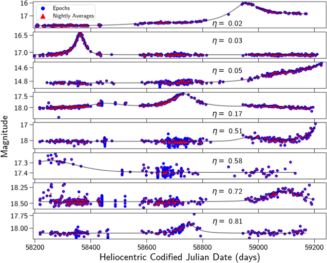
Figure 4. Example simulated microlensing lightcurves and their η values, with individual epochs (blue) and nightly averages (red), with data cut on catflag < 32768. Each model (black line) was generated from distributions set by PopSyCLE simulations throughout the Galactic plane. The models were then injected directly into DR5 lightcurves, enabling calculations and cuts on these lightcurves to represent the diversity of cadence and coverage seen throughout the DR5 data set.
Download figure:
Standard image High-resolution image4.4.2. Computing ηresidual Cut
η and ηresidual were calculated on all simulated microlensing events. Most of the simulated microlensing events had low values of η, due to the correlation between subsequent data points as compared to the sample variance, and high values of ηresidual, due to the lack of correlation after subtracting a successful microlensing model. Figure 5 shows the location of the simulated microlensing events in the η–ηresidual plane.
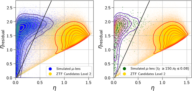
Figure 5. Microlensing events were clearly delineated in the level 2 catalog by calculating η on lightcurves and the residuals of those lightcurves after fitting them to a four-parameter microlensing model. Those data were cut on catflag < 32768. η was calculated on the nightly averages of ZTF candidates (yellow), simulated microlensing lightcurves (blue), and simulated microlensing lightcurves in the black hole search space (green). This measurement of η was made on both the entire lightcurve (x-axis) and on a lightcurve with the four-parameter model subtracted (y-axis). Microlensing events tended toward smaller η values due to their correlated lightcurves and larger ηresidual when microlensing is the only source of variability. This enabled a cut (black line) in this η–ηresidual space that retained 83.6% of simulated events and 95% of black hole parameter space, while removing 98.8% of the ZTF candidates from our sample.
Download figure:
Standard image High-resolution imageFor each level 2 candidate we selected the object with the most nights of observation from among the candidate's objects. The η, ηresidual values of these 7,457,583 best lightcurves are plotted in Figure 5 as well.
There existed a clear distinction between the location of most of our candidates in this plane as compared to the simulated events. This distinction was even stronger when we limited our simulated sample to events with true values of tE > 150 and πE < 0.08. These cuts have previously been used as selection criteria for identifying microlensing events as black hole candidates (Golovich et al. 2022). We ran a grid of proposed cuts with the criteria ηresidual ≥ m · η + b and found that m = 3.62, b = 0.01 retained 83.6% of all microlensing lightcurves and 95% of the black hole microlensing lightcurves, while removing 98.8% of our level 2 candidates. This left us with 92,201 candidates in our level 3 catalog. This cut could be tuned if we were interested in optimizing for a more complete sample of shorter duration events.
4.5. Level 4: Cleaning Data and Cutting on a Seven-parameter Microlensing Model
To avoid spurious results and retain only the cleanest data, here we removed any lightcurve epochs with catflag ≠ 0. We then required that all objects have at least 50 unique nights of good data with this new criteria. This brought us from 92,201 to 90,810 candidates. The nightly averaged magnitudes of the best lightcurve of each candidate were fit with a seven-parameter microlensing model for further analysis. The scipy.optimize.minimize routine (Virtanen et al. 2020) using Powell's method (Powell 1964) was used to fit each lightcurve to a point-source point-lens microlensing model including the effects of annual parallax. The seven free parameters include t0, u0, tE, πE,E, πE,N, FLSN, and bsff as defined in (Lu et al. 2016). The average time to fit each object with this model was 1.2 ± 0.3 s. 578 candidates failed to be fit with this model and were cut. All simulated microlensing events were also fit with this model for comparison. The results of these fits for both populations are shown in Figure 6.
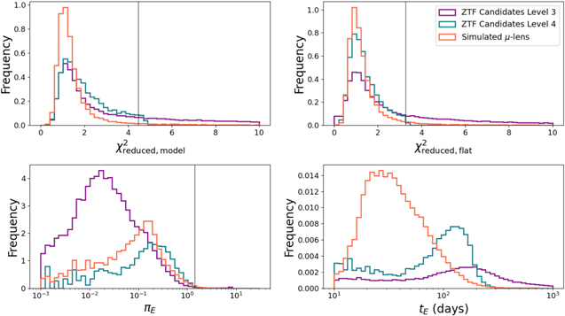
Figure 6. Fitting the seven-parameter model to both level 3 candidates (purple) and simulated microlensing lightcurves (orange) revealed cuts that removed many objects, leaving behind our level 4 catalog (blue). The  of the entire lightcurve that was fit to a microlensing model (top left) had a long tail in the level 3 candidates that was not present in the simulated microlensing events, motivating a cut on the 95th percentile (black line). Similarly, the long tail for level 3 candidates of the
  of the lightcurve outside of t0 ± 2tE fit to a flat model (top right) was not seen in the microlensing samples and was removed with a cut on the 95th percentile. A small number of events with significantly larger microlensing parallaxes (bottom left) were removed with a similar 95th percentile cut. These cuts, and others, removed events with Einstein crossing times (bottom right) longer than are detectable by our survey.
Download figure:
Standard image High-resolution imageSeveral cuts were then made on candidates using these fits. Our first cut was to remove candidates with excessively large  values because they could not be well fit by our microlensing model. We call this
  in Table 3, where opt is an abbreviation for scipy.optimize, to distinguish it from the model fit in Section 4.6. The threshold of
  was set by calculating the 95th percentile of the simulated data and removed 40,856 candidates. We next required that the candidate's selected object had a range of epochs observed equal to at least 2tE nights outside of the event (t0 ± 2tE), removing another 34,522 candidates.
  was determined by calculating the
  comparing the brightness to the average magnitude in the region outside of the fit event for each lightcurve. This statistic and its 95th percentile value were also calculated on the simulated events and candidates above this percentile were removed. A cut was performed on candidates above the 95th percentile of πE to eliminate candidates where excessive parallax was producing variability in the data. Lastly, a cut was applied to t0, limiting candidates to only those that peaked at least 1 tE into the survey data, removing candidates that peaked too early to be well constrained. The combination of these cuts resulted in a list of 8649 candidates that were either completed or ongoing events in our level 4 catalog.
4.6. Level 4.5: Cutting on a Bayesian Microlensing Model
8646 of the 8649 candidates were successfully fit within 12 hr with a nested sampling algorithm to a point-source point-lens microlensing model with annual parallax locked to the sky location of the candidate. We performed this more sophisticated fit to obtain error bars on our microlensing parameter measurements. Gaussian processes were also included in the fitter to model correlated instrument noise using the procedure outlined in Golovich et al. (2022). This fitter fit the three most observed objects within the candidate with at least 20 nights of data to the same model simultaneously. This model had five parameters shared by all lightcurves (t0, tE, u0, πE,E, πE,N), two photometric parameters fit for each lightcurve (mbase, bsff), and four Gaussian process parameters for each lightcurve (σ, ρ, ω0, S0). Therefore, each candidate was fit with either 11, 17, or 23 parameters if it contained one, two, or three objects with at least 20 nights of data. The median time to complete each of these fits was 101, 469, and 1812 s for one, two, or three lightcurves respectively. If more than three lightcurves were in the candidate (due to multiple sources with up to three filters per source), then the three lightcurves with the most nights of data were selected due to computational constraints.
We then cut on the quality of the fit by requiring  for the data evaluated against the model fit. We also required that candidates have observations on the rising side of the lightcurve (t0 − tE ≥ 58,194); this is a re-implementation of an earlier cut with this more rigorous fit. We have 5496 remaining candidates after these cuts. We waited to make the rest of the quality cuts before separating out the ongoing events since they may have poorly constrained parameters.
4.7. Level Ongoing
All of the level 4.5 candidates are interesting objects worthy of further investigation. We divided our sample into candidates with peaks during the survey (t0 + tE ≤ 59,243) and ongoing candidates with peaks after the survey was completed (t0 + tE > 59,243). These subsamples of 3938 peaked and 1558 ongoing candidates, respectively, serve two different purposes. Calculating the statistical properties of microlensing candidates within ZTF data requires a clean sample of completed events. We therefore sought to further remove contaminants from the 3938 candidates that had peaked within the survey (see Section 4.8). The 1558 candidates that had yet to peak need to be further monitored while they are rising in brightness until they reach their peak amplification. At this point, they could be fit with a microlensing model to determine whether they are good events and perhaps even black hole candidates worthy of astrometric follow-up.
4.8. Level 5: Cutting on Completed Events
Data quality cuts were applied to the resulting fits, as outlined in Table 3. The fractional error on tE was required to be below 20% to ensure that a final distribution of Einstein crossing times would be well defined. Cuts on ∣u0∣ ≤ 1.0 and bsff ≤ 1.5 are commonly accepted limits for the selection of high-quality events.
The candidate was required to have 4tE of observations that were outside of significant magnification (t0 ± 2tE), which is a re-implementation of a previous cut with this more rigorous fit. All of these cuts reduced the sample down to 950 candidates in our level 5 catalog. We additionally fit the 1558 candidate to the same nested Bayesian sampler but with only the one single lightcurve containing the most nights of observations. This gave us the error on the t0 and tE measurements that could be used to determine which of these candidates should be astrometrically observed.
4.9. Level 6: Manual Lightcurve Inspection and Cross Reference
There were 950 candidates remaining in the level 5 catalog. There were several failure modes of our pipeline that could only be addressed by manually labeling each of these candidates. To facilitate this, we constructed a website that provided access to the candidate information contained within the PUZLE database tables and lightcurve plots generated by zort. This website is a docker container running a flask application that was served on NERSC's Spin platform. The website connected inspectors to the NERSC databases and on-site storage. Each of the candidate labels was derived after inspecting the data by eye and grouping the candidates into common categories. The description and final number of candidates with each label after manual inspection are outlined in Table 4. Examples of each candidate with each label are shown in Figure 7.

Figure 7. Lightcurves exemplifying the four labels manually assigned to level 5 candidates. Only the clear microlensing events were selected for our final level 6 catalog. The blue point in the upper right corner for each lightcurve represents the average error for each lightcurve. The limitations of our method can be seen in the persistence of non-microlensing variables that had additional variation not explained by microlensing, as well as lightcurves where the model was not supported by the data labeled as poor model/data. The possible microlensing events had insufficient data to be confidently named microlensing. Those appearing to rise in brightness could be confirmed with further observations.
Download figure:
Standard image High-resolution imageTable 4. Microlensing Event Visual Inspection Labels
| Label | Description | Number |
|---|---|---|
| Clear microlensing | Model accurately follows a rise and fall in brightness with a clear region of uncorrelated non-lensing brightness measured outside of the event. | 60 |
| Possible microlensing | Model accurately follows either a rise or fall in brightness, does not have a sufficient area of non-lensing outside of the event, or has fewer than 10 points deviating from the baseline. | 580 |
| Poor model/data | Model predicts a significant variation in brightness in areas without sufficient data. | 229 |
| Non-microlensing variable | Correlated deviation from the model is present in either the non-lensing region outside of the event, or the lightcurve is similar in appearance to a supernova. | 81 |
Download table as: ASCIITypeset image
The inspector was shown a display page with the four labels displayed above the zort lightcurves alongside information from the database. The model derived from the Bayesian fit was plotted onto the one to three objects that contributed to fitting the model and was absent from those objects within the candidate that did not. The user then selected which label best matched the candidate. The user either selected a scoring mode, where the page was automatically advanced to another unlabeled candidate, or a view mode, where the page remained on the candidate after selecting a label. An example page from the labeling process is shown in Figure 8. 66 candidates were assigned the clear microlensing label.

Figure 8. Level 5 candidates were manually screened by a human expert on the PUZLE website. Inspectors were presented with all objects in the candidate star grouped by source. Model curves were plotted on those lightcurves that were included in the Bayesian fit. The maximum a posteriori probability and 1σ error bars of Bayesian fit parameters were also shown. The inspector then assigned one of four labels to the candidate.
Download figure:
Standard image High-resolution imageAfter visual inspection, each of the candidates was checked in SIMBAD to identify if they have some other known source of variability. Five objects were identified as quasars in Sloan Digital Sky Survey (which is expected to be 99.8% complete Lyke et al. 2020) and one was identified as a Be star with significant variability (Pye & McHardy 1983). The summary of the final 60 candidate events can be found in Table 7.
5. Results
Our final catalog of level 6 candidates contains 60 clear microlensing events (see Appendix B, Table 7). The sky locations of these events are shown in Figure 9. 41 (68%) of the events are within the Galactic plane (∣b∣ ≤ 10°) and 19 events (32%) are outside of it. The distribution of events roughly follows the density of observable objects within DR5, also included in the figure. This indicates that our pipeline is finding microlensing events proportional to the stellar density in each part of the sky. A selected number of these events can be seen, divided by sky location, in Figure 10. There are a large number of events located in parts of the sky far outside of the Galactic plane. Microlensing from two spatially coincident stars is far less likely in these regions. We further discuss the possible origin of these events in Section 6. All 60 microlensing events have been posted online for public use (Medford 2021c), following the schema outlined in Table 5.

Figure 9. Identifying our final level 6 candidates by manual inspection produced a list of clear microlensing events scattered throughout the night sky. The 950 level 5 candidates (blue) were positioned throughout the sky (top left), while the 60 level 6 events (red, top right) are primarily located within the Galactic plane (bottom right). 35 of the 60 level 6 events (58%) appear within the area of the PopSyCLE simulations we performed (footprints in green). However, there are a significant number of events at larger Galactic latitudes. This can be explained by the relatively larger number of objects with Nepochs ≥ 20 (with catflag < 32768) observed at these locations in DR5 (bottom left), contamination by long-duration variables, or perhaps the presence of MACHOs in the stellar halo.
Download figure:
Standard image High-resolution image
Figure 10. Our level 6 catalog contains 41 Galactic plane microlensing events (purple) and 19 events outside of the plane (green) ordered by increasing  . These sample lightcurves show the variety of timescales and magnitudes identified by our pipeline. The Galactic longitude and latitude of each event are printed in each corner. These 19 events nearly double the total number of microlensing events yet discovered outside of the Galactic plane and bulge.
Download figure:
Standard image High-resolution imageTable 5. Exported Candidate Schema
| Column Name | Data Type | Unit ID |
|---|---|---|
| String | ⋯ | |
| ra | Float | Degrees |
| dec | Float | Degrees |
| t0 | Float | hMJD |
| t0_err | Float | hMJD |
| tE | Float | Days |
| tE_err | Float | Days |
| u0_amp | Float | ⋯ |
| u0_amp_err | Float | ⋯ |
| piE_E | Float | ⋯ |
| piE_E_err | Float | ⋯ |
| piE_N | Float | ⋯ |
| piE_N_err | Float | ⋯ |
| mag_base_r | Float | Magnitude |
| mag_base_err_r | Float | Magnitude |
| mag_base_g | Float | Magnitude |
| mag_base_err_g | Float | Magnitude |
| mag_base_i | Float | Magnitude |
| mag_base_err_i | Float | Magnitude |
| b_sff_r | Float | ⋯ |
| b_sff_err_r | Float | ⋯ |
| b_sff_g | Float | ⋯ |
| b_sff_err_g | Float | ⋯ |
| b_sff_i | Float | ⋯ |
| b_sff_err_i | Float | ⋯ |
Note. Exported data have been posted online for public use (Medford 2021c).
Download table as: ASCIITypeset image
The distribution of Einstein crossing times in our level 6 events are shown in Figure 11. Short-duration events as short as 1 day are recorded, increasing in number up to a peak at tE ≈ 50 days. At longer durations, there is a decline with no events found at tE ≥ 120 days. Several cuts within our pipeline require significant duration of observations outside of the microlensing event. These constraints, combined with the limited duration of DR5, place a strong upper limit on the timescale of events we can detect. We compare this distribution to previous simulations and other surveys in Section 6.

Figure 11. The Einstein crossing times for the level 6 event catalog across the entire sky (purple) and those found within our simulated PopSyCLE Galactic plane fields (green) appear similar. Each curve peaks at around 50 days. These peaks are at longer crossing times than expected from the observable events contained within the overlapping PopSyCLE simulations (blue) scaled to match the number of ZTF Galactic plane level 6 events. The OGLE-IV Galactic plane fields (black), also scaled to match these events, largely agree with our simulations. However, it also shows the limits of our small sample size and short-duration survey to be able to detect the longest duration events.
Download figure:
Standard image High-resolution imageThe luminosity function of our level 6 events is shown in Figure 12. The magnitude shown is the median baseline magnitude, as determined by our Bayesian fitter, for all lightcurves of the same filter belonging to an event. 58 of the events contain at least one lightcurve that was fit by the Bayesian fitter in the r band, 51 of the events have fit data in the g band, and seven events possess fit i band. All three filters peak in number at 19th magnitude, followed by a sharp decline. Our pipeline appears to be removing events fainter than 19th magnitude. The baseline magnitudes for g-band events also decline but at a slower rate. We compare the r-band luminosity function to the simulation in Section 6.
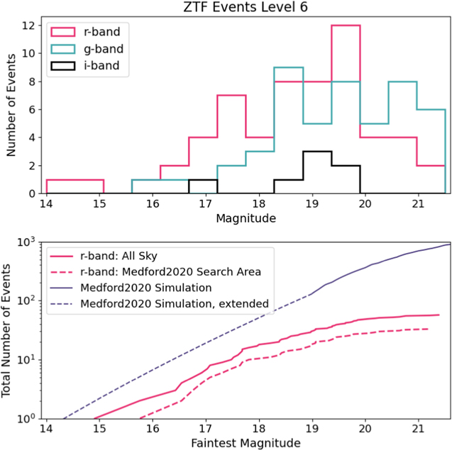
Figure 12. The baseline magnitudes of level 6 events are consistent across filters and follow the shape of the luminosity function predicted by Medford et al. (2020) up to the 19th magnitude. The 60 level 6 events contain 58 r-band, 51 g-band, and seven i-band baseline magnitudes that met the requirements to be fit by the Bayesian fitter. The distribution of these baseline magnitudes (top) appears increasingly plentiful at bright magnitudes, with all three filters dropping off to lower numbers past the 19th magnitude. Comparing the cumulative number of events with r-band baseline magnitudes brighter than a given magnitude (bottom, red) to the Medford et al. (2020) 3 yr l ≥ 10° predictions (purple) show a similar shape for magnitudes brighter than the 19th, but with a clear deficit of events due to the selection effects of our pipeline. At r-band magnitudes fainter than the 19th we are increasingly unable to observe any events. This suggests that executing a search on ZTF data reprocessed to combine images into co-additions could yield many more events as predicted by Medford et al. (2020).
Download figure:
Standard image High-resolution imageMedford et al. (2020) predicted that events observed throughout the outer Galactic plane would have larger source-flux fractions (bsff) than events observed in the Galactic bulge. Figure 13 shows that our level 6 candidates have larger source-flux fractions in line with this prediction. Very few events are seen with bsff ≤ 0.2 as the relatively small stellar densities of the outer Galactic bulge and the stellar halo prevent many neighboring stars from appearing in the instrument's observational aperture. This is in contrast to the findings of most Galactic bulge surveys that find a bimodal distribution with a peak around bsff ≲ 0.2. It is also possible that we may be biased against some high blend events due to the smaller observed change in magnitude. Both g-band and r-band objects have an increasing number of events at larger source-flux fractions and peak at approximately bsff ≈ 1. However, both bands and particularly the g band show an excess of events at bsff ≥ 1. This indicates that there is an overestimation of the background noise present in the photometric measurements. Reprocessing the ZTF observations at the location of these events with calibration parameters tuned to the particulars of each event's fields could improve the estimates of these backgrounds and reduce the number of events with excessive source-flux fractions.
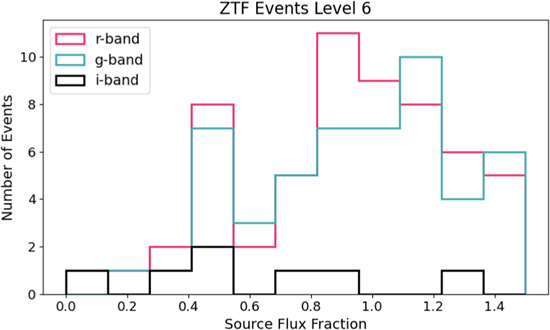
Figure 13. The source-flux fractions of level 6 events drawn from across the sky are more uniform than results drawn from other works aimed toward the Galactic bulge. While the 58 r-band, 51 g-band, and seven i-band baseline magnitudes that met the requirements to be fit by the Bayesian fitter, each have slightly different distributions; they all have very few events with low source-flux fractions (bsff ≲ 0.2). This is expected in the relatively low stellar densities of the outer Galactic plane where the presence of neighboring stars is less prevalent than in the Galactic bulge. The g-band and r-band magnitudes peak at around bsff = 1, where nearly all of the event flux originates in the source. The presence of sources with bsff > 1 indicates that the background is overestimated, indicating the accuracy limits of the DR5 photometric catalogs.
Download figure:
Standard image High-resolution image6. Discussion
Throughout this work we have developed new techniques for efficiently finding events in the massive ZTF data set. Simulations in the same areas of the sky give us expectations against which to compare our results. We also can compare our results to surveys designed specifically for microlensing to get a handle on how well our nontraditional methods have performed.
Our catalog of microlensing events contains objects in regions of the sky where previous microlensing campaigns have not observed. We therefore need to limit our level 6 catalog to a subsample that overlaps with previous OGLE observations and PopSyCLE simulations to be able to make comparisons between tE, πE bsff, and baseline magnitude. The locations of our PopSyCLE microlensing simulations are shown in the right panels of Figure 9. For this comparison we select observable PopSyCLE events that are required to have u0 ≤ 1.0, a maximum amplification Δmr ≥ 0.3, and a baseline magnitude mr ≤ 21.5. These requirements produce events that are observable to ZTF, albeit without a correction for cadence or time span. We then scale the distribution of Einstein crossing times of these events to match the total number of events in our Galactic plane subsample for comparison in Figure 11.
The short-duration slope of our Galactic plane subsample is approximately equal to the simulation. Both our subsample and the PopSyCLE catalogs peak at approximately 50 days. Our subsample mostly agrees above this peak with a potential small excess of long-duration events. Increased ZTF survey time could more than double the microlensing event sample size and either confirm agreement or an excess compared to the simulation. At the longest durations our pipeline is unable to recover events. The cut on sufficient baseline applied to level 4 candidates required 4tE of observations outside of the event (t0 ± 2tE). Applying this requirement for 8tE of data to a 3 yr survey puts an upper limit on our data of t E ∼ 135 days. This explains the sharp drop-off in long-duration events around this point.
Mróz et al. (2020b) conducted the largest Galactic plane search for microlensing events prior to this work, discovering 630 events in the OGLE survey observing 3000 deg2 of the Galactic plane between 2013 and 2019. ZTF observes an even larger footprint of the Galactic plane, with 6900 deg2 between −15° ≤ b ≤ 15° and either 10° ≤ l ≤ 180° or −180° ≤ l ≤ −120°. However, many of these fields point toward or are near the Galactic anticenter where stellar densities are low compared to the Galactic bulge fields observed by OGLE. OGLE also observed their fields for three more years than the ZTF DR5 data set. We include in Figure 11 the distribution of Einstein crossing times found by Mróz et al. (2020b) for the Galactic plane (∣l∣ ≥ 20°), rescaled to match the number of events in our sample. The PopSyCLE and OGLE distributions are in good agreement and predict a relatively equal number of short and long-duration events around a peak of approximately 50 days. While the PopSyCLE fields are run at different Galactic longitudes than the OGLE fields, this is in line with the findings of Mróz et al. (2020b) that the Einstein crossing time distribution within the plane is independent of longitude for ∣l∣ ≥ 20°.
Lam et al. (2020) found that black holes could be identified by placing microlensing events in the tE –πE space and looking for the events with the longest tE and the smallest πE. In Figure 14 we place our events in this space, alongside all observable events from within our PopSyCLE simulations. The simulated events are separated between those with a stellar lens and those with a black hole lens. Level 6 events appear within parameter space most often occupied by events with stellar lenses. This can be caused by several factors. It is possible that all of our events are caused by stellar lenses. The relatively short timescale of DR5 combined with our strict requirements for data outside 2tE of our event also places a limit on the longest events we are able to detect. And finally, small values of πE are difficult to constrain with the quality of photometry that ZTF produces. The result is that we are unable to confidently claim that any of our microlensing events are black hole candidates.

Figure 14. The Einstein crossing times and microlensing parallax of all level 6 events with 1σ errors (red) fall right on top of the region where the PopSyCLE catalogs contain events with stellar lenses (blue). We do not find any events within the region of tE−πE space where PopSyCLE predicts black hole lenses (black). The quality of our data prevents us from constraining small values of πE, and the duration of our survey prevents the detection of the longest duration events. The PopSyCLE events shown are all of the observable events within the simulations.
Download figure:
Standard image High-resolution imageMedford et al. (2020) produced an estimate for the number of events detectable as a function of the faintest observable magnitude of ZTF imagery. They predicted that ZTF would discover ∼500 events in the outer Galaxy for an r-band limiting magnitude of 20.6, and ∼135 events in the same region for an r-band limiting magnitude of 19. In Figure 12 we compare the cumulative distribution function of our luminosity function to these results. Medford et al. (2020) have overpredicted the number of microlensing events discovered by the PUZLE pipeline. The subsample of level 6 events that fall within the Medford et al. (2020) estimated footprint (10° ≤ l ≤ 100°, −10° ≤ b ≤ 10°) has a similar shape to the predictions. However, we detect only 35 microlensing events within the Medford et al. (2020) estimate footprint, 19 of which have mbase,r ≤ 19.
We attribute the gap between the predictions of Medford et al. (2020) and our estimated footprint subsample to several factors. The cut on level 2 candidates removed 16.4% of simulated microlensing events, and the three threshold cuts on level 3 candidates each removed 5% of the remaining simulated events. This accounts for missing 28% of possibly observable events. The level 4 catalog contains all candidates that are well fit by a microlensing model and the cuts applied to them are to get a sample of high-quality events. Therefore, the order of magnitude drop from 5496 candidates to 950 candidates likely removes many true events. Strict requirements on the amount of observable data outside of the event remove long-duration events from the final catalog.
The level 2 and level 3 cuts retained 72% of possible observable events. We selected a random 100 lightcurves from level 4.5 and visually inspected them and found 2% that would have been characterized as clear microlensing, if they had passed to level 5. The 60 events we discovered are 12% of the ∼500 predicted by Medford et al. (2020). We would have to assume that the cuts between levels 3 and 4 removed an additional 81% of true events from our catalog to match these predictions. While this is possible, given that the cuts between levels 3 and 4 selected only the highest quality events from a list of possible microlensing candidates, the difference between our yields and the predictions suggests incompleteness to our method. Medford et al. (2020) did not take into account the effect of gaps in the data due to either weather or seasonality. They also did not cut out events that did not have enough baseline and only required that the peak be in the survey rather than t0 ± tE being in the survey, which may cut out many true events. This makes the discovered number of microlensing events lower than their prediction.
The lack of fainter sources in the level 6 catalog indicates that the ZTF limiting magnitude of 20.6 used in Medford et al. (2020) may have been too large. This result also suggests that our pipeline selectively removed fainter stars with relatively larger photometric errors. This finding also points to the number of additional microlensing events that could be discovered if ZTF were reprocessed by combining subsequent observations into co-additions. Medford et al. (2020) show the nonlinear gains that are predicted to be achieved by this method, and our results corroborate that claim.
M20 and R22 conducted similar surveys of ZTF data for microlensing events (DR2 and through DR5, respectively). They found 30 and 60 events, respectively, 12 and 28 of which we also recovered. The 12 from M20 are also recovered in R22, so we discovered 32 new events. See Appendix A for a more detailed comparison.
6.1. Black Hole Candidates
The level 6 catalog is not ideal for searching for black hole candidates due to the limit on tE that our cuts impose. However, there are numerous microlensing events within ZTF-I that are still ongoing. These were cut in level 4 due to the requirement that all candidates have a time of closest approach within 1tE of the end of DR5 observations. This requirement limits our level 5 and 6 samples to completed events. 1558 candidates that had passed all level 4.5 cuts and t0 + tE > 59243 MJD were classified as level ongoing. If black hole microlensing events are contained within ZTF observations, they would most likely be long duration and therefore still ongoing.
The Einstein crossing times versus times of the closest approach of level ongoing candidates are shown in Figure 15. The majority are modeled to have already passed peak brightness by the end of DR5 data. However, 802 candidates have tE ≥ 150 days and are projected to hit peak brightness during the ZTF-II campaign. These sources could be continuously observed to see if any decline in brightness is in agreement with a microlensing model. If found to do so, astrometric follow-up could be combined with photometric measurement to weigh the mass of the lens and possibly make a detection of an isolated black hole. All 1558 level ongoing candidates have been posted online for public use (Medford 2021c), following the schema outlined in Table 5.
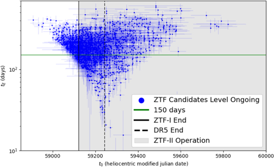
Figure 15. There are 1558 candidates that passed all cuts up to level 4.5 and are still ongoing as of the end of the DR5 data set. They are labeled level ongoing in Table 3. These candidates have a time of closest approach (t0) within one Einstein crossing time (tE) of the end of DR5 observations (black solid line) or later. Events with an Einstein crossing time greater than 150 days (green line) that are continuing throughout ZTF-II (black shaded) are good candidates for continued observation. If they are found to decline in brightness in agreement with a microlensing model, they may be followed up astrometrically to search for black hole lenses.
Download figure:
Standard image High-resolution image
Our search for microlensing in the public data releases was not performed in real time. This approach is limited when attempting to find targets for astrometric follow-up. However, all of our microlensing event selection methods have been designed to be computationally inexpensive and quick to execute.
6.2. Events Outside the Galactic Plane
Our final level 6 catalog contains 19 events outside of the Galactic plane (∣b∣ ≥ 10°), with several examples shown in Figure 10. Previously, attempts to detect microlensing with lenses in the stellar halo by observing background stars in the Magellanic Clouds and the Andromeda Galaxy have yielded only a few events. In Wyrzykowski et al. (2011a) and Wyrzykowski et al. (2011b), the OGLE survey discovered two and three events over 8 yr toward the Large Magellanic Clouds and Small Magellanic Clouds, respectively. Alcock et al. (2000) discovered 13–17 events in the 5.7 yr that the MACHO collaboration observed the Large Magellanic Clouds. Tisserand et al. (2007) detected one event in both the Magellanic Clouds in the 6.7 yr of the EROS-2 survey. Surveys toward the Andromeda Galaxy have detected even fewer events, with Novati et al. (2014) detecting three events over the 4 yr PLAN campaign and Niikura et al. (2019) discovering one short-duration event after 7 hr of dense sampling. Our pipeline's 19 events are more than all 20–25 previously discovered events, nearly doubling the total number of microlensing events discovered outside of the Galactic plane and bulge.
There are several explanations for the presence of microlensing events in significant numbers outside of the Galactic plane in our catalog. The probability of two stars appearing to co-align in lower stellar densities is small, but such yields could be possible by searching across ZTF's all-sky footprint. Our level 4 sample could be contaminated by variations in stellar brightness that are well fit by a microlensing model but are instead other long-duration variability. The contamination is difficult to quantify at this level, as there is simply not enough data to disambiguate the scenarios. However, the level 5 and 6 catalogs should be free of contamination from stellar variability. The most exotic explanation would be the presence of MACHOs that exist in large enough numbers to lens background stars. While previous works claim to have eliminated the possibility of large numbers of MACHOs (Alcock et al. 2001; Wyrzykowski et al. 2011b), more recent simulations that replace a monochromatic mass with an extended mass distribution have reopened the door for MACHOs (Carr et al. 2016; Calcino et al. 2018). Our detections of events toward the stellar halo could be interpreted as evidence for these claims, although further validation is needed.
6.3. Future Improvements
There are several aspects of our pipeline that could be improved to increase the accuracy and yield of our results. Our DR3 to DR5 conversion method leaves out additional i-band observations that would not have been seen in earlier versions. A future implementation could keep an ordered set that tracks the object IDs that have been used and then uses each radec_map to push the new objects into an existing source. We could also do another check of how well the microlensing model fits the lightcurve after fitting more robust models. This could reduce the presence of events with large baseline variability that were classified as non-microlensing variables. We could add a cut to confirm that the peak of the model is covered by the data, as many lightcurves classified as having poor model/data did not have peak coverage. Simulated microlensing lightcurves could have been injected into our sample at the beginning of the pipeline to better measure completeness throughout the process. These lightcurves could also be mixed into the web portal candidates before expert scoring to measure the effect of human bias in identifying clear microlensing events. More careful comparison to simulations after completeness correction would also more accurately assess the effectiveness of our pipeline.
Several large synoptic surveys are due to see first light in the next few years, including the Rubin Observatory's LSST and the Nancy Grace Roman Space Telescope (Roman). The techniques developed in this work are designed to accommodate the massive data sets that these surveys will generate, which will eclipse the size of the largest present-day data sets by orders of magnitude. Our pipeline was designed to remove large numbers of events quickly and without significant computational cost. We fit progressively more complicated models onto the data in order to prevent spending resources fitting events that are less likely to be true microlensing. We eliminate all but the last few candidates before requiring human intervention. This approach, successfully executed on ZTF data, can unlock the potential for the next generation of massive all-sky surveys to become microlensing machines. LSST will be similar to ZTF in terms of sky coverage and cadence. 4 However, for Roman, substantial modifications will have to be made to the pipeline to account for the large temporal gaps between the Galactic bulge observing windows. The ultimate goal is for identification and classification of microlensing events from large surveys to be fully automated, completely free from the intervention of a human expert. This will allow us to more readily review a data set orders of magnitude larger than in this paper, ensure reproducibility, and avoid human error. Using machine-learning methods to accomplish this is an active area of research, especially approaching the era of the Roman Space Telescope's Galactic Bulge Time Domain Survey and the Vera C. Rubin Legacy Survey of Space and Time (Wyrzykowski et al. 2015; Godines et al. 2019; Mróz 2020; Zhang et al. 2021; Gezer et al. 2022).
We thank Antonio Rodriguez and Przemek Mróz for alerting us to the need to use the catflag = 0 criteria. We thank the referee for helpful comments that improved the clarity of the paper. This work is based on observations obtained with the 48 inch Samuel Oschin Telescope and the 60 inch Telescope at the Palomar Observatory as part of the ZTF project. This research used resources of the National Energy Research Scientific Computing Center, a DOE Office of Science User Facility supported by the Office of Science of the U.S. Department of Energy. We acknowledge support from the DOE under grant DE-AC02-05CH11231, Analytical Modeling for Extreme-Scale Computing Environments. J.R.L. and C.Y.L. acknowledge support by the National Science Foundation under grant No. 1909641 and the National Aeronautics and Space Administration (NASA) under contract No. NNG16PJ26C issued through the WFIRST (now Roman) Science Investigation Teams Program. C.Y.L. also acknowledges support from NASA FINESST grant No. 80NSSC21K2043.
Appendix A: Comparison to Rodriguez et al. (2022) and Mróz et al. (2020b)
Rodriguez et al. (2022, hereafter R22) also searched the ZTF data through DR5 for microlensing events and found 60 events. However, only 28 objects in our sample overlapped with theirs, so we made 32 new detections. Of the 32 objects we found that R22 did not, 12 were outside of the ∣b∣ < 20° area they searched. Mróz et al. (2020b, hereafter M20) searched through DR1 and found 30 events, 12 of which overlapped in our pipeline.
Table 6 summarizes where the 32 and 28 objects R22 and M20, respectively, identified that were cut in the PUZLE pipeline. Overlapping events refer to events cut that were in both R22 and M20. Five and four events, respectively (two of which overlap) were cut by the PanSTARRS1 star-determination score, which was necessary in the PUZLE pipeline since we considered objects outside the Galactic plane. Six and five (three of which overlap) were not able to be fit by the four-parameter model fit, and nine and two were cut by not passing the ηresidual cut. These may be because the PUZLE pipeline always fits the band with the most data, whereas R22 fit the r band. Some visually inspected events appear to have outliers in the g band or some variability in the baseline, which may have caused the fit or the ηresidual cut to fail. Two and three (one of which overlaps) events either had the peak start before the survey began or after it ended (t0 ± tE in the data). The equivalent cut in R22 uses t0 ± 0.3tE which may cause the difference. One event in R22 did not pass the  cut. Four events in R22 did not pass the fractional tE error cut for which R22 does not have an equivalent cut. One event in both R22 and M20 did not pass the ∣u0∣ cut. Two and one events (one of which overlaps) did not have enough baseline data, which is important for characterization. Two events (overlapped in both catalogs) were determined not to be microlensing in the by-eye characterization. 226524_5543 is missing data in its peak, but there is some rise and fall so it was put in the possible microlensing category, and 214154_4399 has characteristics of supernovae, including a sharp rise and a slower fall and the r-band data falling above the model.
Table 6. Version of Table 3 with Relevant Cuts and Candidate Events from R22 and M20 to Demonstrate Where in the PUZLE Pipeline the Candidates Would Have Been Cut Out
| Cut Performed | R22 Cands | M20 Cands |
|---|---|---|
| Remaining | Remaining | |
| Cands in paper | 60 | 30 |
| PS1-PSC ≥0.645 | 55 | 26 |
| Successful four-parameter model fit | 49 | 21 |
| ηresidual ≥ η ∗3.82 − 0.077 | 40 | 19 |
| Seven-parameter fit: t0−tE ≥ 58,194 | 39 | 16 |

| 38 | 16 |
| t0 + tE ≤ 59,243 | 37 | 16 |

| 33 | 16 |
| ∣u0∣ ≤ 1.0 | 32 | 15 |
| 4tE baseline outside of t0 ± 2tE | 30 | 14 |
| Manually assigned clear microlensing label | 28 | 12 |
Note. We recover 28/60 of R22 events and find one in the ongoing catalog, and we recover 12/30 of M20 events. See Appendix A for a detailed discussion.
Download table as: ASCIITypeset image
One other object of note is ZTF18absrqlr. Two ZTF data brokers, Fink (Möller et al. 2020) and ALeRCE (Sánchez-Sáez et al. 2021), mark its R.A. and decl. as 28384059, 574372, but it is 307149376, 22830478 in R22 and M20. The coordinates 307149376, 22830478 are duplicated in M20 between ZTF18abnbmsr and ZTF18absrqlr. We believe that R22 actually discovered ZTF18abnbmsr, as we did, and that the ZTF ID is a typo. In Table 6, we treated it as having coordinates 28384059, 574372 in M20 and 307149376, 22830478 in R22.
Appendix B: Summary of the Level 6 Events
Table 7 summarizes the 60 Level 6 candidate events ordered by baseline magnitude.
Table 7. Summary of the 60 Level 6 Candidate Events Ordered by Baseline Magnitude
| puzle ID | ℓ(deg) | b (deg) | R.A. (deg) | Decl. (deg) | mbase | ZTF ID |
|---|---|---|---|---|---|---|
| 206883_29398 | 38.01100 | −6.11373 | 290.61721 | 1.70650 | 14.32 ± 0.00 | ZTF18abaqxrt |
| 226244_24695 | 133.60050 | −4.54272 | 32.49736 | 56.69314 | 14.91 ± 0.00 | ZTF21aalljap |
| 213100_12775 | 52.73575 | −2.90082 | 294.83615 | 16.14483 | 15.76 ± 0.00 | ZTF18abibobd |
| 226146_9143 | 89.38878 | 12.39568 | 301.31815 | 55.32261 | 16.43 ± 0.00 | ZTF20abbynqb |
| 199814_8384 | 14.10087 | 2.38621 | 271.84240 | −15.54738 | 16.76 ± 0.00 | ZTF19abbwpl |
| 211087_11025 | 41.40802 | 8.11634 | 279.40461 | 11.20061 | 16.92 ± 0.00 | ZTF19aaekacq |
| 213871_3211 | 66.29863 | −19.29724 | 316.81620 | 18.13759 | 17.03 ± 0.00 | ZTF19aacmpke |
| 219115_17109 | 73.66961 | −4.80719 | 309.03411 | 32.72093 | 17.08 ± 0.01 | ZTF19aavnrqt |
| 216020_13108 | 60.31419 | 1.48227 | 294.73270 | 24.89685 | 17.31 ± 0.00 | ZTF18abjnrmm |
| 215639_28569 | 57.62132 | 4.06236 | 290.83245 | 23.77312 | 17.48 ± 0.00 | ZTF20abkyuyk |
| 208826_2418 | −61.55329 | 69.64089 | 191.28933 | 6.82385 | 17.52 ± 0.00 | ZTF18acnokyi |
| 198333_4452 | −40.86573 | 42.90427 | 205.29821 | −18.39670 | 17.61 ± 0.01 | ZTF19aarihyl |
| 221243_1676 | 85.63918 | −9.07047 | 322.66138 | 38.85054 | 17.65 ± 0.01 | ZTF20abicdkm |
| 223737_470 | 150.23484 | −6.02984 | 55.43845 | 47.60916 | 17.68 ± 0.00 | ⋯ |
| 200772_6200 | 21.83300 | −9.02418 | 285.98402 | −13.92945 | 17.68 ± 0.00 | ZTF18abmoxlq |
| 204396_25713 | 29.37656 | −2.38778 | 283.36662 | −4.25183 | 17.81 ± 0.00 | ZTFJ1853.5-0415 |
| 199420_23799 | 17.46218 | −5.58708 | 280.80561 | −16.29913 | 17.92 ± 0.01 | ZTF19abqueuo |
| 229329_2194 | 143.55312 | 35.15946 | 132.46388 | 70.66061 | 17.96 ± 0.01 | ZTF19adbtqgz |
| 215476_198 | −170.52767 | 5.21321 | 96.61807 | 23.22059 | 18.00 ± 0.00 | ⋯ |
| 203599_7926 | 26.58814 | −1.75180 | 281.52435 | −6.44398 | 18.13 ± 0.01 | ZTF19aargwsl |
| 198045_37053 | 12.53102 | −2.35737 | 275.42456 | −19.19178 | 18.22 ± 0.01 | ⋯ |
| 227712_653 | 138.73891 | 3.95527 | 48.69432 | 62.34347 | 18.37 ± 0.01 | ZTF19aabbuqn |
| 215341_28211 | 64.60030 | −9.23556 | 307.14936 | 22.83048 | 18.39 ± 0.00 | ZTF18abnbmsr |
| 198550_16292 | 17.54506 | −9.86895 | 284.86976 | −18.10769 | 18.43 ± 0.01 | ZTF20aawxugf |
| 207262_13818 | 34.15426 | 2.63134 | 281.07346 | 2.28667 | 18.53 ± 0.02 | ZTF19aaimlse |
| 227808_6978 | 96.97033 | 45.32348 | 234.62998 | 62.48028 | 18.57 ± 0.02 | ZTF21aazeazr, ZTF20aaljffg |
| 220863_6930 | 69.57788 | 10.90194 | 290.01643 | 37.43482 | 18.61 ± 0.02 | ZTF20aavmhsg |
| 229865_2362 | 141.03852 | 30.61447 | 119.55902 | 73.78493 | 18.74 ± 0.01 | ZTF19adceqzb |
| 224227_29874 | 93.23237 | −2.93470 | 324.57735 | 48.47926 | 18.76 ± 0.00 | ZTF20abvwhlb |
| 204386_5100 | 28.60496 | −1.06885 | 281.83689 | −4.33811 | 18.88 ± 0.01 | ZTF19aavndrc |
| 205166_6377 | 26.80213 | 6.92269 | 273.90054 | −2.25697 | 18.97 ± 0.01 | ZTF19aaonska |
| 205621_17625 | 32.19706 | −1.09287 | 283.49719 | −1.15227 | 18.98 ± 0.02 | ZTF19aaxsdqz |
| 216370_6986 | 60.09199 | 3.08836 | 293.06192 | 25.48256 | 19.06 ± 0.01 | ZTF20abmxjsq |
| 206452_5009 | 34.18144 | −2.37119 | 285.53940 | 0.03010 | 19.07 ± 0.01 | ZTFJ1902.2 + 0001 |
| 213011_4595 | 29.87173 | 42.93640 | 242.37401 | 16.01123 | 19.28 ± 0.01 | ZTF19aasbpld |
| 222741_5669 | 86.49219 | −3.55857 | 318.26336 | 43.33765 | 19.33 ± 0.01 | ZTF19abftuld |
| 225310_3105 | 81.71923 | 22.43713 | 280.73170 | 52.45385 | 19.37 ± 0.01 | ZTF19abbyebj |
| 221496_7115 | 72.90355 | 8.32557 | 294.84456 | 39.17829 | 19.38 ± 0.01 | ZTF20abrtvbz |
| 197737_7136 | 46.67683 | −68.20361 | 350.26232 | −20.17373 | 19.38 ± 0.02 | ZTF20acbdmhy |
| 205225_28572 | 31.55493 | −3.71994 | 285.54582 | −2.91912 | 19.43 ± 0.01 | ZTF19acctqyc |
| 201592_4317 | 23.84423 | −7.34805 | 285.33834 | −11.40450 | 19.45 ± 0.02 | ZTF18absjezs |
| 225706_1669 | 133.87116 | −6.45141 | 31.94920 | 54.79037 | 19.52 ± 0.01 | ⋯ |
| 209120_548 | 120.81612 | −55.66621 | 11.65688 | 7.18577 | 19.62 ± 0.01 | ZTF18abwamwf |
| 198940_35883 | 14.27337 | −1.33996 | 275.33980 | −17.17655 | 19.63 ± 0.03 | ⋯ |
| 210144_774 | 22.08289 | 40.47883 | 242.13879 | 9.70584 | 19.72 ± 0.02 | ZTF20aawghfe |
| 225914_13362 | 99.04746 | −0.46726 | 329.19298 | 54.09859 | 19.75 ± 0.01 | ZTF18aayhjoe |
| 210677_14481 | 42.48555 | 3.54901 | 284.04933 | 10.11678 | 19.78 ± 0.01 | ZTFJ1856.2 + 1007 |
| 204863_2897 | 34.50146 | −11.49132 | 293.81041 | −3.83897 | 19.84 ± 0.01 | ZTF20aawijop |
| 219013_4366 | 62.12153 | 15.97480 | 280.73453 | 32.87309 | 19.86 ± 0.01 | ZTF19aamrjmu |
| 206800_23883 | 29.59880 | 10.33983 | 272.14526 | 1.77291 | 19.96 ± 0.02 | ZTF20abagzwt |
| 203625_1402 | 28.59530 | −4.97245 | 285.32605 | −6.11747 | 20.01 ± 0.03 | ⋯ |
| 201089_14825 | 17.00608 | 4.44172 | 271.43912 | −12.01451 | 20.18 ± 0.02 | ZTF18ablrdcc |
| 215636_7171 | 56.73376 | 4.52214 | 289.93921 | 23.20425 | 20.26 ± 0.01 | ZTF20acbmtwd |
| 222375_11305 | 72.03940 | 17.58765 | 283.26664 | 42.29320 | 20.51 ± 0.03 | ⋯ |
| 219134_11822 | 77.28109 | −9.13134 | 315.71335 | 32.81170 | 20.65 ± 0.05 | ZTF19acbptvn |
| 201147_4625 | 20.90054 | −4.85962 | 281.72420 | −12.91335 | 20.70 ± 0.03 | ZTF19abijroe |
| 227178_28049 | 101.10161 | 4.66963 | 326.17312 | 59.37792 | 20.81 ± 0.02 | ZTF18aaztjyd |
| 218269_30320 | 64.29643 | 6.23607 | 292.17602 | 30.66463 | 21.21 ± 0.03 | ZTFJ1928.7 + 3039 |
| 229949_8332 | 104.65664 | 24.98626 | 286.18769 | 73.45821 | 21.25 ± 0.06 | ZTF20aaymulz |
| 227822_8865 | 92.34280 | 34.10588 | 260.41834 | 62.87877 | 21.38 ± 0.04 | ZTF19abgvmln |
Note. More extensive parameters of the events can be found online at Medford (2021c).
Download table as: ASCIITypeset image
Footnotes
- 3
Additional details about the content and structures of products in these data releases can be found at https://www.ztf.caltech.edu/ztf-public-releases.html.
- 4