


Abstract
Some of the most energetic pulsars exhibit rotation-modulated γ-ray emission in the 0.1–100 GeV band. The luminosity of this emission is typically 0.1%–10% of the pulsar spin-down power (γ-ray efficiency), implying that a significant fraction of the available electromagnetic energy is dissipated in the magnetosphere and reradiated as high-energy photons. To investigate this phenomenon we model a pulsar magnetosphere using 3D particle-in-cell simulations with strong synchrotron cooling. We particularly focus on the dynamics of the equatorial current sheet where magnetic reconnection and energy dissipation take place. Our simulations demonstrate that a fraction of the spin-down power dissipated in the magnetospheric current sheet is controlled by the rate of magnetic reconnection at microphysical plasma scales and only depends on the pulsar inclination angle. We demonstrate that the maximum energy and the distribution function of accelerated pairs is controlled by the available magnetic energy per particle near the current sheet, the magnetization parameter. The shape and the extent of the plasma distribution is imprinted in the observed synchrotron emission, in particular, in the peak and the cutoff of the observed spectrum. We study how the strength of synchrotron cooling affects the observed variety of spectral shapes. Our conclusions naturally explain why pulsars with higher spin-down power have wider spectral shapes and, as a result, lower γ-ray efficiency.
1. Introduction
In γ-ray pulsars a significant fraction of the spin-down power (between 0.1% and 10%) is converted into high-energy photons (Abdo et al. 2013). This suggests that somewhere in the magnetosphere the Poynting flux radiated by the rotating star is efficiently dissipated and converted into the energy of pairs populating the magnetosphere and, ultimately, to γ-rays. The equatorial current sheet beyond the light cylinder, where magnetic reconnection takes place, is a likely candidate where this energy extraction can take place. The emergence of the current sheet in plasma-filled magnetospheres of neutron stars was predicted in the force-free (FF) formulation (Contopoulos et al. 1999; Gruzinov 2005; Timokhin 2006), while kinetic plasma simulations permitted them to be modeled self-consistently, capturing the process of magnetic reconnection (Chen & Beloborodov 2014; Philippov & Spitkovsky 2014; Belyaev 2015; Cerutti et al. 2015; Kalapotharakos et al. 2018; Cerutti et al. 2020). Two-dimensional simulations of axisymmetric magnetospheres were able to achieve significant separation of scales between the macroscopic extent of the current layer and the microscopic plasma-kinetic scale. However, the dynamics of a 2D reconnecting current sheet may be different from that in three dimensions. Current layers in three dimensions are prone to kinetic instabilities, such as the kink instability, which may disrupt the layer, interfering with the magnetic reconnection and tearing instability, and potentially leading to the suppression of dissipation rate (Guo et al. 2021; Werner & Uzdensky 2021; Zhang et al. 2021). Neutron stars that have magnetic axes misaligned with respect to their rotation axes have intrinsically nonaxisymmetric magnetospheres and, as a result, more complex structures of current layers, which can only be studied in three dimensions.
In global 3D simulations, large-scale separation is numerically challenging and expensive, and yet critically necessary to resolve the hierarchical chain of plasmoids that occur in the magnetic reconnection and mediate the particle acceleration process. As a result, while previous 3D simulations properly capture the general structure of the magnetosphere, the complex dynamics of the current layer is still largely unexplored due to the rather limited scale separation in prior works. In this work we make an attempt to properly capture the microphysics of the current sheet in 3D particle-in-cell (PIC) simulations by extending the separation of macro-to-microscales to ≳100. We achieve this by employing a hybrid approach for particle pushing in our simulations, where the motion of particles in highly magnetized regions is reduced to that of their guiding centers, while in the accelerating regions, the full motion is recovered (Bacchini et al. 2020). This approach also enables us to include a strong self-consistent synchrotron radiation-reaction force acting on the subsect of particles for which gyration is resolved.
The goal of the present work is to quantify the amount of magnetic energy dissipation, determine which plasma parameters control the average and the maximum energy that particles gain during the acceleration process, and what role the strong synchrotron cooling, present in most of the energetic pulsars, plays. We begin in Section 2 with a brief introduction to the 3D structure of the magnetosphere, and the numerical setup we employ. We then describe the energy dissipation process in the reconnecting current layer and demonstrate that the rate of this process controls the overall dissipation rate in the magnetosphere (Section 3). In Section 4 we study the particle acceleration and high-energy radiation in the regimes of dynamically strong and weak synchrotron cooling. Section 5 summarizes our main findings, putting them in the context of Fermi observations. In particular, we show how the interplay of radiative losses and particle acceleration in magnetic reconnection explains the observed diversity of γ-ray spectra.
2. Plasma-filled Pulsar Magnetospheres
Pair cascade near the neutron star surface has long been thought to populate the neutron star magnetospheres with pair plasma (Sturrock 1971; Ruderman & Sutherland 1975). When the magnetosphere has enough plasma supply, ne ≳ ρGJ/∣e∣, its structure relaxes to the FF solution, where the electric field component parallel to the magnetic field vanishes everywhere, E · B = 0. Charge density necessary to sustain FF solution is called the Goldreich–Julian (GJ) density, ρGJ = Ω · B /(2π c) (Goldreich & Julian 1969). For the most energetic pulsars, pair-producing cascade is highly efficient and can populate the magnetosphere with pair multiplicities up to ne ∣e∣/ρGJ ∼ 104 (Timokhin & Harding 2015, 2019). In this work we only consider neutron star magnetospheres with the abundant pair plasma supply, where deviations from the FF solution are at the scale of the local plasma skin depth, de .
2.1. Numerical Setup
We employ radiative PIC algorithm implemented in the Tristan-MP v2 code designed by Hakobyan & Spitkovsky (2020) to simulate the 3D dynamics of the entire magnetosphere. Synchrotron radiation drag force is included in the equations of motion for particles in the Landau–Lifshitz form. The magnitude of the force is artificially enhanced with respect to the Lorentz force, so the most energetic particles lose a substantial amount of energy on the gyration timescales. A similar approach for modeling synchrotron drag has been used in previous works (e.g., Cerutti et al. 2016).
Our simulations start with an empty Cartesian domain of the size , where RLC = c/Ω is the light cylinder of the magnetosphere, and Ω is the spin frequency of the neutron star. The star itself is modeled as a perfectly conducting rotating sphere in the center of the domain (similar to Philippov et al. 2015). A dipolar magnetic field is imposed as a boundary condition near the surface of the sphere, as well as the initial condition in the whole domain. The angle between the magnetic axis and the rotation axis is further denoted by χ. Near outer boundaries, all of the electromagnetic field components are damped to zero, and the particles are allowed to leave. Particle distribution is sampled on average by ∼10 macroparticles per grid cell (PPCs), with fewer PPCs farther from the star. 6 To mitigate the numerical artifacts from finite PPCs, we employ digital filtering of the deposited currents with a stencil of size 2. We also tested the setup with a lower-resolution simulation and 10 times more PPCs, arriving at the same results.

To fill the magnetosphere with plasma we mimic the pair-production process near the surface of the star by injecting pair plasma in a small spherical shell of size Δr at a rate proportional to the local GJ density: Δn(θ, ϕ)/Δt = finj∣ρGJ(θ, ϕ)/e∣(c/Δr). The dimensionless parameter finj controls the injection multiplicity. The exact value of this number is unimportant, as long as enough plasma is injected to establish the FF solution (we typically set finj = 1). We also give a marginal initial velocity to the newly injected particles along the local magnetic field lines (typically a Lorentz factor of γ ≈ 2). 7
To be able to resolve the plasma skin depth, de , everywhere except for the surface of the star, we greatly reduce the scale separation compared to realistic pulsars. The radius of the star is resolved by 75Δx (we will denote Δx as the size of the grid cell), while the size of the light cylinder is RLC ∼ 440Δx (or ∼6 times the radius of the star). The strength of the magnetic field at the surface, B*, which also rescales the Goldreich–Julian density, is chosen in such a way that , where is the plasma skin depth near the light cylinder. The scale separation between macroscopic and microscopic (plasma-kinetic) length scales is, thus, at most ∼200 in our highest-resolution simulation (see almost 8 orders of magnitude scale separation in realistic pulsars). Large separation of scales ensures that the growth of microscopic plasma instabilities that develop at kinetic timescales (inverse plasma frequency, ) is much faster than the dynamical timescale characterized by the rotation period, P. Localized 2D simulations (see, e.g., Werner et al. 2016) show that at scale separation ≳100, kinetic instabilities establish an asymptotic regime, which justifies our choice of . The choice of these parameters yields the total size of the simulation domain (2200Δx)3.


In regions where the magnetic field is strong (close to the surface of the star), we significantly underresolve particle gyration timescale (ωB Δt/γ ≫ 1, where ωB = ∣e∣B/me c, and γ ≈ few). To avoid associated numerical errors, we employ a coupled guiding-center/Boris algorithm for solving particle equations of motion (Bacchini et al. 2020). This approach allows us to ignore gyrations of most of the particles in the bulk of the magnetosphere where the gyration is underresolved, reducing their motion to that of their guiding centers. At the same time, switching to conventional Boris pusher in regions where E/B > 0.95 allows us to recover the full equation of motion for high-energy particles in regions with vanishing magnetic field (i.e., current sheets). 8 By ignoring the synchrotron drag force for particles in the guiding center regime, we can also avoid having numerical errors in the strong cooling regime, when the synchrotron cooling algorithm heavily relies on the resolution of gyration orbit.
Overall, the three dimensionless parameters that we fix independently in our simulations are:
- 1.: the ratio of the size of the light cylinder and the plasma skin depth at a corresponding GJ plasma density. We refer to this as the scale separation of our simulation;
- 2.R*/Δx ≈ 75: the number of simulation cells per stellar radius, which we call the resolution of our simulation; and
- 3.RLC/R* ≈ 6: the size of the light cylinder, w.r.t. the size of the star.

In addition we also have the obliquity angle, χ, which we vary from 0°–90°, and the cooling strength, which we detail below.
2.2. Steady-state Numerical Solution
In all of our simulations, after a brief transient lasting for about one rotation period of the star, P, a steady-state structure is established that closely resembles the FF solution. The snapshot of the steady-state for the neutron star with an inclination angle χ = 30° is outlined show in Figure 1. Plasma close to the surface corotates with the neutron star, flowing along almost poloidal magnetic field lines that start and end at the surface of the star. This corotation extends up to RLC = c/Ω from the rotation axis (Ω being the rotation frequency of the neutron star), the light cylinder. Outside the light cylinder, plasma can no longer corotate with the star, and pairs slide along spiral magnetic field lines beyond the RLC, moving almost radially outward. While in the inner magnetosphere (inside the light cylinder), the magnetic field is almost purely poloidal, in the outer magnetosphere it has a toroidal components.

Figure 1. Poloidal slice of the 3D plasma density normalized to from a simulation of an inclined rotator with χ = 30° (here is the GJ density near the pole of the star). The surface of the neutron star and its rotation axis are shown in blue. Magnetic field lines traced from the surface of the star, as well as the direction of the magnetic moment, are shown in green. The light cylinder, RLC, shown with white dashed lines, separates the inner magnetosphere from the outer magnetosphere and the wind. The current sheet originating near the Y-point and spreading into the outer magnetosphere is clearly visible.


Download figure:
Standard image High-resolution imageThe rotation of the magnetosphere imposes a poloidal electric field in the wind zone, Eθ ∼ Bϕ . As a result, the pulsar radiates electromagnetic energy in the form of a radial Poynting flux: . This flux, integrated over a sphere that encloses the light cylinder, is the spin-down energy of the neutron star, often denoted as , which for an aligned rotator reads:


where B* is the magnetic field strength near the stellar surface at the equator.
Opposing field lines from the northern and southern hemispheres of the neutron star are divided in the outer magnetosphere by a current sheet. The structure of the equatorial current sheet is more visible in the simulation with no obliquity, shown in Figures 2(a), (b) (hereafter we refer to this simulation as R75_ang0, since χ = 0°, and R* = 75Δx). 9 Cartesian coordinates are normalized to the RLC, and (0, 0, 0) is the middle of the box, where the center of the neutron star is. Figure 2(a) shows the slice of the simulation in the x = 0 plane, while Figure 2(b) shows the slice in the z = 0 plane (in this simulation, χ = 0°). Color indicates the plasma number density compensated by the cylindrical radius squared, its value is normalized by the corresponding GJ density at the surface of the star times the radius of the star squared, .


Figure 2. (a): poloidal slice of the plasma density from a simulation of an aligned rotator (R75_ang0, after two full rotations of the neutron star). Magnetic field lines originating at the stellar surface are shown with green lines. White dashed lines indicate the light cylinder. (b): equatorial slice of the plasma density. As in (a), green lines show the direction of the magnetic field. The white dashed circle corresponds to the light cylinder. Blue arrows trace the direction of the equatorial current in the equatorial sheet. Ripples in density are caused by the combined effect of two instabilities (tearing and kink) in the current sheet. In the slice (a), the drift-kink instability of the current sheet is apparent. Slight collimation of field lines near the boundaries close to the poles in (a) is caused by imperfect absorbing boundary conditions in the aligned case. This feature, not present in simulations of misaligned pulsars, however, does not affect the global solution, or the dissipation in the current sheet.
Download figure:
Standard image High-resolution imageFrom Figure 2 it is evident that the total plasma density close to the current sheet is few to ten times larger than the local GJ density, which means the magnetosphere has enough plasma to screen the accelerating electric field almost everywhere. If the parallel electric field were screened everywhere, magnetic energy dissipation in the magnetosphere would not be possible, and the integral in Equation (1) would be constant with r, , yielding no γ-ray emission.

The accelerating electric field can survive in microscopic subregions of the equatorial current sheet. The characteristic scale of these regions does not exceed a few-to-tens of plasma skin depths, de = c/ωpe, where ωpe is the plasma frequency for relativistic electron-positron pairs in the current sheet. For the Crab pulsar, this parameter close to the light cylinder is of the order of a few centimeters. The light cylinder, on the other hand, is almost 8 orders of magnitude larger (for the Crab, it is ∼1500 km). To properly model the dynamics of these subregions, first-principles PIC simulations are necessary.
3. Dissipation of Spin-down Energy
The structure of the magnetosphere in PIC, as was demonstrated in the previous section, is very similar to that in FF. This should come as no surprise, since in our simulations E ∥ is perfectly screened with abundant plasma, and magnetized particles follow field lines everywhere except for the equatorial current sheet where the magnetic field vanishes. The key difference from FF solutions is the dynamics of the current sheet. In ideal FF, the energy dissipation in the current sheet is due to the finite resolution of the grid, and is thus numerical in its nature. PIC algorithm, on the other hand, enables us to "resolve" this dissipation on plasma-kinetic scales, by capturing the reconnection of magnetic field lines from first principles.
3.1. Kinetic Instabilities in the Current Sheet
The equatorial current sheet highlighted in Figure 2 is not laminar even in the aligned case, χ = 0°. Rather, it is prone to kinetic instabilities that develop on microscopic timescales comparable to . Drift-kink instability displaces the current sheet in the z-direction, which results in the undulation of the sheet at a certain saturated amplitude (shown in the poloidal slice of Figure 2(b); also see Philippov & Spitkovsky 2014; Cerutti et al. 2015). The wavevector of this perturbation is perpendicular to the local magnetic field and is parallel to the local current.

More importantly, the current sheet also experiences tearing instability due to relativistic reconnection of magnetic field lines from the upstream (see, e.g., Cerutti & Philippov 2017; Philippov & Spitkovsky 2018; Cerutti et al. 2020). As a result of this process, magnetic islands ("plasmoids") are formed containing hot plasma energized in the reconnection process. In-between the plasmoids, there are magnetic nulls—regions where the magnetic field lines tear, and energy dissipation happens, the "x-points."
Figure 3(c) shows a 3D rendering of the plasma density as well as two slices of the same quantity: one along the magnetic field lines (Figure 3(a) indicated with a red surface in panel 3(c)), and the other one—perpendicular to field lines, along the direction of the current (Figure 3(b) indicated with a blue surface). In Figure 3(b) one can see the undulation of the current sheet due to drift-kink instability. The reconnection of magnetic field lines and tearing instability, on the other hand, are better visible in Figure 3(a); overdense regions in the sheet are the plasmoids, which, in 3D, look like tubes elongated almost radially (Figure 3(c)).
Figure 3. Three-dimensional rendering of the plasma density (compensated by r2) from a simulation of an aligned rotator (R75_ang0). The 3D rendering (panel (c)) is accompanied by two slices ((a) and (b), also visible in three dimensions as red and blue surfaces). One of the slices (a) is orthogonal to the equator and curves along the upstream magnetic field lines, while the second one (b) is along the direction of the current perpendicular to the magnetic field. Overdense elongated tubes in panel (c) are the 3D flux ropes, the plasmoids, which are produced as a result of the nonlinear tearing instability. In a 2D slice, (a) the dynamics of both the current sheet and the plasmoids look very similar to those in isolated current sheet simulations. In panel (b) the drift-kink instability is visible, which deforms the current sheet in the direction perpendicular to the direction of the tearing instability. An animated version of this figure is available and at https://youtu.be/-YXJ4yTlhWw. In the animation, the camera rotates around the Z-axis, corotating with the star, for several rotation periods. The duration of the animation is 23 s.
(An animation of this figure is available.)
Download figure:
Video Standard image High-resolution imageThe dynamics of the reconnecting current sheet in Figure 3(a) is very similar to a 2D Harris sheet, except for the fact that the upstream plasma moves along the magnetic field lines with bulk Lorentz factor (in reality, this is expected to be see, e.g., discussion by Cerutti et al. 2020). 10 In Figures 4(a) and (b) we take the slice along the upstream magnetic field lines (similar to Figure 3(a)) where we plot quantities crucial for understanding the energy dissipation in the current sheet: the vertical component of the E × B drift velocity in units of c, and the energy dissipation rate, j · E . In the upstream (above and below the current sheet), the plasma motion is strictly constrained by magnetic field lines, which coincide with the plane of Figures 4(a) and (b). Cold plasma and opposing magnetic field lines are brought together by an drift (shown in Figure 4(a)); the current sheet then becomes unstable and tears producing plasmoids (shown with magenta contours). The dimensionless rate of inflow is set by the reconnection; this value can be directly measured from the simulations. For our simulations, this value is close to


where the subscript "in" corresponds to the velocity component directed into the current sheet. This value is consistent with isolated 2D/3D simulations of the Harris sheet, and has been demonstrated to be independent of any numerical or physical parameters (such as the number of macroparticles per cell, the resolution, or the extent of the box; see, e.g., Werner et al. 2018).

Figure 4. Two panels show different quantities in the same slice as Figure 3(a). Panel (a) shows the E × B inflow rate into the current sheet; this corresponds to the rate at which the reconnection of magnetic field lines occur, roughly, βrec ∼ 0.1. In panel (b) we plot the work done by the electric field (compensated by rxy 3), which also indicates the electromagnetic energy dissipation rate. The latter is localized in the thin equatorial current sheet. On both panels we overplot the plasmoids in magenta (their boundaries are selected as contours of large overdensities clearly visible in Figure 3(a)).
Download figure:
Standard image High-resolution image3.2. Magnetic Energy Dissipation via Reconnection
Reconnecting magnetic field in the current sheet generates a nonideal electric field in the direction of ∇ × B , which is the direction of the current in Figure 2(a) (in Figures 3(a) and 4(a) and (b), this corresponds to the out-of-plane direction). The magnitude of the nonideal electric field is of the order of Erec ∼ βrec Bup, where Bup is the magnetic field strength in the upstream. Because of the emergence of j · E (shown in Figure 4(b)), some of the Poynting flux radiated by the star (Equation (1)) dissipates in the magnetosphere. As seen in Figure 4(b), dissipation is concentrated exclusively in the thin current sheet outside the light cylinder, where the energy of the electromagnetic field is converted into the kinetic energy of plasma through magnetic reconnection. According to Poynting's theorem:

This means that L(r) is constant within the light cylinder, r < RLC (where j · E = 0), but decays with radius for r > RLC. Figure 5 shows L(r) from one of our simulations with χ = 0° computed using the flux of the Poynting vector (blue line), and the volume integral of j · E (red line). The orange band corresponds to an analytical model described further in this section.

Figure 5. Dissipation of the Poynting flux in the outer magnetosphere from a simulation of an aligned rotator. The blue line is the direct measurement of the Poynting flux vs. r for two different simulations: R75_ang0 (solid line), where , and R60_ang0 (dashed line), where . The red line shows the j · E , which accounts for the dissipation rate of the electromagnetic energy. The orange band is the theoretical fit, Equation (5), with βrec ≈ 0.09–0.12. L0 is computed from Equation (1). A slight increase of L with respect to L0 in the inner magnetosphere is due to the fact that the Y-point in our simulation is slightly inside the r/RLC = 1; this leads to slightly more open field lines and thus more Poynting flux. Weak synchrotron cooling of the particles is present in both of these simulations; however, as we show further, the effect of cooling on the reconnection rate in this high-magnetization regime is negligible.


Download figure:
Standard image High-resolution imageTo understand the slope of L(r) beyond the light cylinder, it is useful to build a simple analytical model of the Poynting-flux dissipation in the current sheet. For χ = 90° rotator this model has been studied by Cerutti et al. (2020); here we focus on χ = 0°. As mentioned earlier, the dissipation of Poynting flux in our simulations is caused by the work done by the reconnection electric field, j · E , as described by Equation (3). The strength of the electric field generated due to magnetic reconnection at a given distance r from the star is Erec(r) ∼ βrec Bup(r). Here, the reconnecting magnetic field is a combination of poloidal and toroidal components above and below the current layer, , the value of which beyond the light cylinder can be approximated as (rotating monopole; see, e.g., Deutsch 1955 and Michel 1973). Here and further, . Since (4π/c) j = ∇ × B , the current generated during reconnection can be estimated as j ∼ cBup/(2π δcs), where δcs is the characteristic width of the current sheet. Thus, the volume integral in Equation (3) reduces to:


The integral over the polar angle, θ, at each r is accumulated in a small region near the equator (θ = π/2) of angular size Δθ ∼ δcs/r (which is the current sheet highlighted in Figure 4(b)). 11 Integrating Equation (4) then yields

where we also used . The logarithmic term in this expression corresponds to the dissipation of toroidal field, Bϕ , while the second term corresponds to the dissipation of poloidal field, Br . At large distances, r ≫ RLC, the first term prevails, as the field is almost purely toroidal. However, for the small region, RLC < r < 2RLC, where γ-ray emission likely originates, contributions from both terms are important. In Figure 5 we plot the total Poynting flux, L, across a spherical shell of radius r (blue line). The orange band in Figure 5 corresponds to Equation (5) with βrec varying from 0.09–0.12 (this number can be directly measured from Figure 4(a)). From the plot, it is evident that about 10% of the radiated Poynting flux, L0, is dissipated in the outer magnetospheric current sheet within the first RLC. The magnetic field strength weakens with distance, and particles can only radiate (via synchrotron) in the gigaelectronvolt range within the first one-to-few RLC. Thus, the measured γ-ray luminosity, Lγ , should be directly correlated with the energy dissipated in this narrow range of radii. 12 The precise value of the dissipated energy, as we have demonstrated above, is only determined by the reconnection rate at plasma microscales.

As we demonstrate in the next section, in our simulations, the plasma in the upstream part of the current sheet moves along the magnetic field lines with relativistic velocities of Γ ∼ 10. Naively, one would expect that since the rate of reconnection is universally defined in the proper frame of the upstream, in the lab frame the measured rate should be Γ times slower. Nevertheless, we do not observe any significant change in βrec ∼ 0.1 (similar observations have been made by Cerutti et al. 2020). To check the consistency of this result in a more controlled way, we performed local 2D simulations of the current sheet, where the upstream plasma was initialized with a relativistic velocity component along the unreconnected magnetic field. From these simulations, we find that the global reconnection rate in a given reference frame is controlled by the strength of the electric field in the x-points, which are at rest. Despite the motion of the upstream, the reconnection rate remains constant, as long as the outflow velocities from the x-points remain relativistic. This condition is satisfied as long as the characteristic Alfvén four-velocity in the current sheet is much larger than the square root of the bulk four-velocity of the upstream, Γ: . 13 For realistic pulsar parameters, the particle four-velocity, Γ, which (close to the light cylinder) is mostly along the magnetic field lines, is of the order of 10–100, while the magnetization is close to 105–106. This means that the reconnection is unlikely to slow down because of the bulk motion of the upstream.

For other values of χ, our results are consistent with earlier works (PIC: Philippov et al. 2015; and MHD: Tchekhovskoy et al. 2013). Namely, the spin-down luminosity near the light cylinder , and for larger values of χ, we see inhibited dissipation in the current sheet, as the jump of the magnetic field across the current sheet is balanced primarily by the displacement current (as opposed to the conduction current) for larger inclinations (see, e.g., Philippov & Spitkovsky 2018).

Some of the previous 2D axisymmetric simulations of aligned pulsars (Belyaev 2015; Hu & Beloborodov 2022) reported the presence of excess dissipation near the Y-point, at the level of a few percent of L0, with a lower dissipation rate at r > RLC. While the reduced dissipation rate is caused by the fact that in 2D simulations only one of the magnetic field components can be reconnected (only the poloidal one), the anomalous dissipation near the Y-point has unclear origins. In our 3D simulations, we also see signs of excess dissipation in the Y-point, but only in the aligned case, and only when the skin depth near the light cylinder is marginally resolved (dashed blue line in Figure 5). 14
The electromagnetic energy dissipated during the reconnection in the current sheet is deposited into plasma particles. In the next section, we focus on particle energization in the current sheet and its consequences for the observed high-energy emission in γ-ray pulsars.
4. γ-Ray Emission
Relativistic magnetic reconnection is known to produce nonthermal particle population (Guo et al. 2014; Sironi & Spitkovsky 2014; Werner et al. 2016); reconnection in the current sheets of neutron star magnetospheres is no exception. These energized particles are believed to radiate via synchrotron mechanism, producing the pulsed high-energy emission observed in γ-ray pulsars (Cerutti et al. 2016; Philippov & Spitkovsky 2018). However, the synchrotron drag, the strength of which depends on the value of the magnetic field outside the current sheet, can inhibit the acceleration process, greatly affecting the outgoing photon spectrum.
4.1. Dynamical Importance of Synchrotron Drag
In the current sheets of pulsar magnetospheres, the synchrotron cooling timescale for particles is always much shorter than the system-crossing timescale, characterized by the rotation period. However, it can be comparable to the acceleration time of the highest-energy particles, meaning that the relative importance of cooling can be significant at microscopic timescales. The efficiency of cooling can be conveniently quantified with a dimensionless number γrad. This number corresponds to the Lorentz factor of particles for which the synchrotron drag force in the given background magnetic field B is comparable to the Lorentz force from the reconnection-driven electric field E ∼ βrec B. This condition reads: , where σT is the Thomson cross section. 15 Particles with γ ≫ γrad will lose their energies while being exposed to a perpendicular magnetic field component much faster than they are able to accelerate; the opposite is true for particles with γ ≪ γrad. Notice that strictly speaking this is not applicable to particles at x-points, since the magnetic field vanishes there.

The main parameter that determines the characteristic maximum energy to which particles accelerate during reconnection is the magnetization of the upstream (unreconnected) plasma, σ. For a given background magnetic field, B, and number density of inflowing plasma, n, this dimensionless parameter is equal to twice the ratio of the magnetic energy density and the rest mass energy density of plasma:

where B and n are measured in the proper frame, where plasma is at rest. In Figure 6 we show the magnetization parameter in the upstream of the reconnecting equatorial current sheet in a poloidal slice. In our typical simulations, magnetization of the upstream, σLC, is close to 500–1000, as shown with a vertical slice in Figure 6(b). This parameter, which in relativistic reconnection is always ≫1, determines the characteristic maximum energy to which particles can be accelerated in a single x-point (or x-line in three dimensions; see Figure 4(b)). If secondary reacceleration is prohibited, the nonthermal distribution function of accelerated particles extends at most to energies of a few times σ me c2. Energized particles, however, may either then reenter the current sheet or become trapped in plasmoids and get accelerated again via secondary processes to even higher energies (Petropoulou & Sironi 2018; Hakobyan et al. 2021; Zhang et al. 2021). However, as we demonstrate below, in pulsar magnetospheres with realistic parameters, this process is suppressed due to synchrotron losses.

Figure 6. (a): plasma magnetization parameter, σ, in a poloidal slice of the simulation R75_ang0_gr2 with weak synchrotron cooling ( subscript gr2 corresponds to ). A 1D slice of the σ across the current sheet is shown in panel (b). Magnetization of the upstream is close to 103, where the background plasma density . Magnetic field lines are shown by green in panel (a).


Download figure:
Standard image High-resolution imageLater in this section we will refer to the case when γrad < σ as the strong cooling regime, while the opposite case will be referred to as the weak cooling regime. The value of γrad (close to the light cylinder) only depends on the magnetic field strength: , which we know rather reliably for pulsars by extrapolating the magnetic field strength at the surface. The magnetization, σLC, on the other hand, depends on plasma density near the light cylinder, which is harder to constrain. However, we can estimate that approximately, by assuming that the cutoff frequency of the γ-ray photons corresponds to the synchrotron peak energy for the highest-energy particles with Ee ∼ 4σLC me c2, . This provides a rough empirical estimate for σLC, which for the population of γ-ray pulsars varies between 105 and 106. Consequently, the reconnection in the current sheets of pulsars proceeds in the marginally radiative regime, where . In the next section we quantitatively investigate how the electromagnetic energy dissipation rate, as well as the particle distribution and synchrotron spectra, change depending on the ratio .


4.2. Particle Acceleration and Synchrotron Spectra in the Radiatively Cooled Magnetosphere
In our simulations, we keep σ ≫ 1 in the outer magnetosphere (to ensure the reconnection proceeds in the ultrarelativistic regime), and vary the ratio γrad/σ. Following the discussion earlier, this ratio determines the relative importance of the effects of synchrotron cooling on reconnection dynamics, and, as we demonstrate later, results in qualitatively different high-energy radiation spectra. In Figure 7 we show snapshots from simulations with three different inclination angles, χ = 0°, 20°, and 60° (three rows), comparing two extremes of the cooling efficiency in each case: no cooling (left column, panels (a), (c), and (e)), and strong cooling (right column, panels (b), (d), and (f)). In the same snapshot we also plot the integrated Poynting flux, L, as a function of radius with the x-axis corresponding to the radius in RLC (shared with the x-axis of respective snapshots). We find that the general structure of the current sheet is largely unaffected by the strength of the synchrotron cooling. At low inclination angles, χ ≲ 20°, the current sheet is more intermittent with stronger cooling (compare Figure 7(a) and Figure 7(b)), but at higher inclinations, the difference is negligible. The rates of magnetic reconnection and, as a result, the Poynting-flux dissipation curves, L(r), are only marginally affected by the cooling strength for all values of χ.


Figure 7. Density snapshots from late stages (more than two rotations) of six different simulations with varying obliquity angle, χ, and synchrotron cooling efficiency, . All of the slices are in the poloidal plane. Rows correspond to, respectively, χ = 0° ((a) and (b)), 20° ((c) and (d)), and 60° ((e) and (f)). Simulations in the left column ((a), (c), and (e)) have synchrotron cooling turned off, while the ones on the right ((b), (d), and (f)) have very strong synchrotron cooling, . Each panel also contains 1D plots of L(r)/L0 (white line; L0 is the flux measured at r = 0.75RLC) with horizontal axes, r, having the same scale as the x-axes of snapshots. Green bands correspond to the dissipation due to reconnection estimated by Equation (5) with the rate varying between 0.8 and 0.15.


Download figure:
Standard image High-resolution imageWe further closely inspect two simulations with χ = 20° and χ = 60° (these simulations will be referred to as R75_ang20, and R75_ang60; all of the other parameters except for the inclination angle are the same as in R75_ang0). In the first series of runs, we keep σLC ≈ 500–1000 and vary to capture the following regimes: (where γrad = ∞ corresponds to a simulation without synchrotron cooling; for future reference, we denote these simulations as R75_ang20_gr1o15, R75_ang60_gr1o15, ..., R75_ang60_grINF).


Particle distribution functions in the current sheet are also very similar for all of the values of the cooling strength, as shown in Figures 8(a) and (c). In all of the studied cases, particles in the layer are able to accelerate to γ ∼ σLC in x-points, forming a power law of f ∝ γ−1 − γ−2 (for larger values of χ = 60°, the spectrum steepens from γ−1 to about γ−1.3). Only in the most strongly cooled simulation do we see that the cutoff of particle distribution is slightly shifted toward lower energies. This marginal difference is likely an effect of comparably small-scale separation in our simulations, and will most likely be unnoticeable for realistic systems. In weakly cooled simulations above γ > σLC, we see a smooth transition to γ−2.5 − γ−3 and, eventually, to an almost exponential cutoff. Naively, one would expect that in the reconnection process with strong cooling, particles cannot gain energies higher than γrad me c2; however, in reality, the cooling becomes faster than the acceleration for these particles. As mentioned above, this is not necessarily true, as the acceleration takes place in the region of the current sheet where there is virtually no cooling (this has also been demonstrated in 2D simulations by Cerutti et al. 2014; Kagan et al. 2016; Hakobyan et al. 2019, etc.). On the other hand, in the strong cooling regime, once particles leave the accelerating regions (either back to the upstream or into plasmoids), they very quickly lose their energies without a chance to get reaccelerated again to energies larger than a few σ me c2. As a result, the nonthermal distribution of particles, even in the case of a very strong cooling, is determined by the acceleration at x-points and extends up to γ ∼ few σ (see, e.g., Sironi 2022).

Figure 8. Panels (a) and (c) show particle spectra and panels (b) and (d) photon spectra for the R75_ang20, and R75_ang60 simulations in different synchrotron cooling regimes. Effective σ at the light cylinder is marked with yellow stripes. Three smaller bars of different colors in panels (a) and (c) indicate the effective γrad. The color bar at the top of both panels puts particle energies into correspondence with synchrotron peak energies, E ∝ γ2 BLC. Photon energies are normalized to . While particle spectra look almost identical (except for the strongest cooled case), peaks of photons are shifted to smaller energies for smaller γrad/σ. Only particles in the current layer are accounted for. Simulations without synchrotron cooling (black lines) are not shown in panels (b) and (d), since we do not collect photons in that case.

Download figure:
Standard image High-resolution imageIn Figures 8(b) and (d), we show the spectra of emitted synchrotron photons for both χ = 20° and χ = 60° simulations for different cooling strengths. In all cases, we see a recurring pattern in photon spectra: a rise ν Fν ∝ ν, a transition with a peak and a decay at higher energies. The power-law index for the distribution of photons is roughly consistent with the power-law index for the distribution of particles, i.e., f ∝ γ−p leads to ν Fν ∝ ν−(p−3)/2.
Since the majority of the particles are unable to retain energies γ > γrad (and since σ > γrad), the spectral peak in photon energies, Ep, roughly corresponds to the synchrotron emission of particles with γ ∼ γrad: . This is evident from a comparison of the color bars in Figure 8(a), (b): we see a shift of the emission peak toward lower energies for simulations with stronger cooling. The spectrum, nevertheless, extends farther, as particles are still able to accelerate to energies >γrad in the x-points, albeit rapidly radiating away. In the case of moderate-to-weak cooling (σ < γrad), the majority of particles is accelerated to γ ∼ σ, and the peak is controlled by the value of σ: (see green lines in Figure 8(b), (d)).


Note that we do not capture significant intermittency at higher energies for the strong cooling simulation, which was prominent in 2D localized simulations by Hakobyan et al. (2019). Because of this, simulations with stronger cooling also have a smaller spectral cutoff energy together with a smaller spectral peak, despite the fact that the cutoff in particle distribution is unaffected. In two dimensions, the high-energy intermittency, which was responsible for extending the cutoff to values close to ℏ ωB σ2, was primarily caused by merger events of plasmoids of different sizes varying from just a few to hundreds of plasma skin depths. In our global 3D simulations, plasmoids are at most several skin depths in size, and there is only a handful of them in the current sheet. This striking difference in the separation of scales between local 2D and global 3D simulations, as well as the overall complexity in the structure of the current sheet in three dimensions, may explain the observed difference. Future large-scale localized 3D simulations of magnetic reconnection in the high-σ strong cooling regime will be able to clarify this conflict and provide a more definitive picture.
4.3. Effects of Additional Pair Loading
To test how particle acceleration and radiation spectra change with the value of magnetization, σLC, we artificially load the current sheet with extra plasma to alter the effective value of σ in the current layer (see Figure 9). For each pair injected from the surface, we initialize M − 1 additional pairs at rest in the cyan region shown in Figure 9. 16 All of the other parameters, such as and Vpc ≈ 5000 me c2, are kept constant. These "secondary" pairs rapidly catch up with the bulk E × B outflow, and their ultimate effect is the decrease of the effective magnetization ∼M times (as shown in the left panels of Figure 9).


Figure 9. Plasma density, compensated for the falloff with the distance, , for three simulations R75_ang0 with different pair loading rates. The additional injection region is highlighted with cyan. Newly created particles are initialized with zero velocity. From top to bottom, M = 1 (no extra injection, all particles originate at the surface), M = 2 (one particle is injected per each surface-injected particle), M = 20. To the left of each panel, we plot the magnetization of the steady-state solution for each case as a function of vertical coordinate (the corresponding slice is shown with a white dashed line).

Download figure:
Standard image High-resolution imageIn Figure 10 we show corresponding particle distributions in the current layer, as well as the emerging radiation spectra for all of these simulations. The blue line shows the fiducial case without additional injection. In that simulation the magnetization is σLC ∼ 103, and particles in the current layer form an extended power law of f ∝ γ−1 extending to γ ∼ σLC. In this moderate cooling regime, the peak of the radiation spectrum corresponds roughly to the synchrotron peak of the particles with . With increasing pair density, M, magnetization at the light cylinder drops proportionally (as shown with the red and green lines in the particle spectra of Figure 10). In the cases of M = 2 and M = 20, the magnetization values near the Y-point are, respectively, σLC ≈ 500 and ≈50. Particles form a clear hard power-law distribution up to γ ∼ σLC with a steepening to f ∝ γ−2 − γ−3 at higher energies, γ > σLC, followed by a cutoff. In these cases, pairs are still able to accelerate to energies >σLC me c2 since the cooling is weak (). In the simulation shown with a dashed green line, we inhibit this secondary acceleration by enhancing the synchrotron cooling strength (decreasing to ≈200). These simulations clearly demonstrate that the particle acceleration potential of the pulsar outer magnetosphere is indeed determined by the local magnetization parameter, , rather than the electric potential drop near the polar cap, Vpc/me c2, defined in equation Equation (A1). In pulsars these values are correlated, with σLC being significantly smaller:


where is the plasma multiplicity near the light cylinder.


Figure 10. Particle energy distributions in the current layer and photon spectra for simulations shown in Figure 9. The dashed lines indicate the effective magnetization near the light cylinder, σLC, and the corresponding photon energies, . We also show an additional simulation (with a dotted line) where we enhance cooling for the M = 20 case by decreasing γrad ≈ 200. In all of the other cases, the cooling strength is fixed at γrad ≈ 1000. Photon energies are normalized to .


Download figure:
Standard image High-resolution imagePhoton spectra in these runs are consistent with our earlier predictions (see Section 4.2). In the first run (blue line) the spectral peak is set by particles with energies . When we decrease σLC (while keeping the cooling strength, , constant) we see that the peak is only marginally sensitive to σLC (which drops from 103 in M = 1, to 200 in M = 2, and to 50 in M = 20), and is controlled by particles with (hence the similarity of the red and green curves). When we decrease to 200 for the σLC ∼ 50 run (green dashed line), the peak is shifted toward lower energies (despite the fact that particle distributions are only marginally affected).


5. Discussion
5.1. Summary
In this work we closely inspect 3D PIC simulations of neutron star magnetospheres with the strong synchrotron radiation-reaction force included. Our primary focus is the energy dissipation and the plasma dynamics in the reconnecting current sheet. To be able to properly capture the kinetic physics governing the energy extraction in the current layer, we push the separation of macro-to-microscales in our simulations to ∼200.
We show that the rate of plasma inflow into the reconnecting equatorial current sheet, which is controlled by plasma kinetics at the scales of microscopic x-lines, determines the dissipation rate in the entire magnetosphere. This puts a stringent constraint on how much electromagnetic energy can be dissipated (and, ultimately, radiated) in the current layer within a few light cylinders. From simulations we find that this dissipation rate is almost insensitive to both the bulk motion of the background unreconnected plasma, and the synchrotron cooling strength, as long as the magnetization is high: σLC ≫ 1. The fraction of the dissipated energy within the region between RLC < r < 2RLC in the outer magnetosphere varies between 1% and 10%, with the exact value depending only on the pulsar inclination angle.
Due to the fast synchrotron cooling timescale, reconnection in the equatorial current layer proceeds in the radiatively efficient regime. A large fraction of the dissipated electromagnetic energy is radiated away by the accelerated pairs. Since cooling is always faster than the dynamical time of the current sheet, the amount of radiated energy is insensitive to the cooling strength and only depends on the amount of magnetic energy dissipated.
We confirm that the particle distribution is almost unaffected by synchrotron cooling, with particles in the current sheet forming a hard power-law spectrum with steep cutoff at energies of ∼σLC me c2. Photon spectra, on the other hand, are evidently different. In the marginal cooling regime, , both the peak and the high-energy cutoff of the emission are controlled by the magnetization parameter, . In the magnetospheres where synchrotron cooling is strong, , plasmoids that carry the bulk of the plasma and contribute to the high-energy emission the most quickly cooled down to the characteristic temperatures of (see, e.g., Uzdensky & Spitkovsky 2014). Our simulations suggest that the peaks of the emission are thus controlled by the synchrotron emission of particles with energies comparable to Te : .


5.2. Observational Implications
Observations by the Fermi telescope during the last decade have shown that some of the pulsars with erg s−1 emit in γ-rays with characteristic luminosities ranging between 0.1% and 10% of the spin-down power. Our 3D PIC simulations provide strong evidence that this emission is powered by magnetic reconnection in the equatorial current sheets of pulsar magnetospheres. Reconnection occurs in the nonlinear stage of the tearing instability, which develops in the equatorial current sheet on microscopic timescales, , where wcs is the characteristic width of the sheet, and is the bulk Lorentz factor of the upstream plasma in the wind. 17 The width of the current sheet, wcs, is defined by the pressure equilibrium, and is set by the Larmor radii of particles with characteristic Lorentz factors of : , where the parameter is set by radiation-reaction force. In this paper we explicitly assumed that the plasma microphysics is disentangled from the large-scale structure of the pulsar magnetosphere by taking a large enough separation of micro-to-macro scales. For this assumption to be valid, it is necessary for the tearing instability to develop much faster than the dynamical time of the magnetosphere—the pulsar rotation period, Ω−1. The ratio of these timescales is always large for γ-ray pulsars, , meaning that at least for the young pulsars with erg s−1, the reconnection develops almost instantly in the current sheet near the Y-point. 18


The amount of energy dissipation within a few light cylinders beyond the Y-point, where the high-energy radiation originates, is determined by the reconnection rate, βrec ≈ 0.1, and the pulsar inclination angle. Importantly, we find that this rate is not suppressed by the presence of the bulk flow of the upstream plasma along the magnetic field lines, as long as the Lorentz factor of the Alfvén velocity is larger than that of the bulk flow, . 19 In young pulsars , whereas , implying that the two are separated by at least an order of magnitude. However, even when (which might be the case for the older pulsars with erg s−1), our findings indicate that the rate is only marginally slower (by a factor of 2 at most), which is virtually unnoticeable for the purposes of observations.


Our simulations demonstrate that the dissipated power is further radiated away via synchrotron radiation, which we identify as the main emission mechanism in our simulations. Curvature radiation in this context is negligible (contrary to what has been reported by, e.g., Kalapotharakos et al. 2018), as the dynamically strong cooling prevents particles from accelerating to energies beyond σLC me c2, and the Larmor radii of the most energetic particles, ρL , are limited to microscopic plasma scales, . For the Vela-like pulsars, where the discharge near the polar cap is the main source of pairs, and there is no additional pair production in the current sheet, most of the dissipated energy is emitted directly in the form of the highest-energy synchrotron photons around one to a few gigaelectronvolts, leading to characteristically high values of . The youngest Crab-like pulsars, on the other hand, produce a sufficient amount of high-energy photons, so that pair creation near the light cylinder becomes an important source of additional pair plasma (Lyubarskii 1996; Hakobyan et al. 2019). To estimate the fraction of the dissipated magnetic energy that goes into these secondary pairs, we need to evaluate the effective optical depth for the γ-ray photons, τγ x = fγ x σT nx RLC, where fγ x ≈ 0.25 (given by the maximum cross section of the pair-production process: see, e.g., Akhiezer & Berestetskij 1965), and nx is the number density of X-ray photons, the presence of which is required for the gigaelectronvolt photons to pair produce. 20 The effective number density of the low-energy photons can be estimated as , where Lx is the luminosity in X-rays, and εx is the characteristic energy of X-ray photons. The pair-production cross section is the largest for the photons that satisfy (here, εγ ≈ GeV). Substituting all of the values, and taking , which is the case for the youngest pulsars (Marelli et al. 2011), we finally find: . For the Crab, erg s−1, and we find that τγ x ≈ 1. The relatively large value for the optical depth means that the nonnegligible fraction of the dissipated energy is deposited into secondary pairs produced in the reconnection upstream. Characteristic energies of the produced pairs can be estimated as , where Eγ ≈ 0.1–1 GeV is the characteristic energy of the pair-producing photons. For the Crab, , and the synchrotron emission of these secondary pairs corresponds to energies .


The maximum energy to which particles accelerate during the reconnection process is controlled by the plasma magnetization parameter near the light cylinder, few-to-ten σLC, which in turn determines the cutoff energy in the observed emission. The synchrotron cutoff can be expressed as , where (see, e.g., Cerutti et al. 2016), and γcut ≈ few · σLC. For reconnection in the strong cooling regime, most of the dissipated energy is radiated away via emission from the highest-energy pairs. The dissipation power is equal to ∣e∣Erec c, where Erec ≈ βrec BLC, while the synchrotron radiation power is . From the definition of , we may then find: , where BLC is the upstream magnetic field strength. Substituting this into the expression for the cutoff energy yields: . The cutoff energy is then uniquely set by the ratio , resulting in . For Vela-like pulsars, κ ≈ 103 − 104 (Timokhin & Harding 2015), erg s−1, resulting in Ecut ≈ 1–10 GeV. 21


For the most energetic Crab-like pulsars with a strong magnetic field near the light cylinder (BLC ∼ 4 × 10⁶ G for Crab), pair creation near the Y-point and beyond is important. The amount of produced pairs is proportional to the optical depth, τγ x , estimated earlier, and the number of gigaelectronvolt photons. The production rate can be estimated as , where εγ ≈ GeV. To obtain the multiplicity κ, we compare this with the GJ flux, , where we assumed that the is equal to the GJ current: . We then find the multiplicity of pair production near the light cylinder . For the Crab pulsar, , and yielding κLC ≈ 106. For the Vela, on the other hand, , and yielding κLC ≈ 3 (similar to what has been obtained by Lyubarskii (1996). 22 Substituting κ ≈ κLC for the Crab to the relation for the cutoff energy, we then find Ecut ≈ 0.1–1 GeV.


To reiterate, while the amount of the dissipated magnetic energy is uniquely set by the microphysics of the reconnection and the inclination angle, the luminosity of the observed emission can be somewhat different between the high- Crab-like, and the low- Vela-like pulsars. The cutoff energies are dictated by the highest-energy pairs, and in both cases, the numbers are close to the observed one to a few gigaelectronvolts. Spectral peaks, on the other hand, are different. In the case of Vela-like pulsars, most of the dissipated Poynting flux is radiated away via synchrotron at energies close to the cutoff around 1–10 GeV. For the Crab-like pulsars, however, secondary pair production near the light cylinder is important, and a large fraction of the dissipated energy goes into pairs that further re-radiate via synchrotron at a range of energies spanning all the way to kiloelectronvolts, resulting in a much broader spectrum. This yields a smaller γ-ray luminosity in the Fermi band (between 0.1 and 100 GeV), which is clearly observed by Abdo et al. (2013), who reported beyond erg s−1.


5.3. Future Work
In our simulations we did not include self-consistent pair production (neither the γ B → e± process near the polar cap, nor the γ γ → e±, Breit-Wheeler, process near the light cylinder), instead choosing to provide a constant inflow of plasma from the surface of the star. Our reasonable assumption was that as long as enough plasma is provided to the magnetosphere (n ≳ nGJ), its general structure, as well as the dynamics of the current layer would not depend on how exactly the plasma was supplied. However, as mentioned earlier, for the youngest Crab-like pulsars, the secondary pairs produced by the two-photon pair production in the outer magnetosphere can carry a large fraction of the dissipated energy, re-radiating it at optical to X-ray frequencies. Additionally, as was shown in 2D simulations of an isolated current sheet (Hakobyan et al. 2019), and as mentioned in Section 4.3 of this paper, these secondary pairs inhibit the acceleration process during reconnection, thus controlling the extent of the γ-ray signal. To understand this process in more details, and also study the intermittency, the light curves, and the polarization characteristics of the distinct X-ray signal these pairs produce, global 3D simulations with proper two-photon pair-production physics are necessary. The Tristan-MP v2 code (Hakobyan & Spitkovsky 2020), used in this paper, supports the capabilities of tracking individual photons and modeling their interaction pair by pair. In the future we plan to apply this capability, coupled with the hybrid guiding center particle pusher, to model the pair-production process and its dynamics in the global context of the magnetosphere more realistically. While we think our main conclusions outlined in Section 5.2 will still hold, these more robust simulations will allow us to more self-consistently predict the optical/X-ray luminosity for the young pulsars (which we simply postulated empirically for the purposes of our estimations), to understand the long-term evolution of the secondary pairs, as well as their effect on the structure of the pulsar wind.
The authors would like to thank Andrei Beloborodov and Ioannis Contopoulos for insightful comments and thorough remarks, as well as the anonymous reviewer for concise and helpful comments. This work was partially supported by the U.S. Department of Energy under contract No. DE-AC02-09CH11466. The United States Government retains a nonexclusive, paid-up, irrevocable, world-wide license to publish or reproduce the published form of this manuscript, or allow others to do so, for United States Government purposes. This work was supported by NASA grant 80NSSC18K1099 and NSF grants AST-1814708 and PHY-1804048. A.S. is supported by Simons Investigator grant 267233. Computing resources were provided and supported by Princeton Institute for Computational Science and Engineering and Princeton Research Computing. This research was facilitated by Multimessenger Plasma Physics Center (MPPC), NSF grant PHY-2206607.
Appendix A: Numerical Setup and Limitations
In this Appendix we present some dimensionless relations both in the context of astrophysical pulsars, and our simulations. We discuss how each of these parameters is up/down-scaled in our global simulations relative to realistic values.
Consider a rotating perfectly conducting neutron star with a radius R* and a magnetic moment , where B* is the magnetic field strength near the equator. For simplicity let us consider χ = 0°, i.e., the magnetic moment is aligned with the rotation axis. If the magnetosphere is filled with enough plasma to provide the necessary charge density for screening the parallel electric field, then magnetic field lines that originate inside a circular region of radius Rpc around the magnetic axis will be open, i.e., will continue to infinity. This region, the polar cap, has a radius of , where RLC = c/Ω is the light cylinder of the neutron star. The electric field generated at the surface of the star across the polar cap generates a potential drop, Vpc, which can be written in a dimensionless form:


where is the nominal gyrofrequency at the surface of the star, and P is the rotation period of the star.

Defining the plasma multiplicity close to the light cylinder, λ, as nLC = λΩBLC/2π c∣e∣, the scale separation (ratio of the light cylinder to the plasma skin depth) in the magnetospheric current layer is given by the following expression:

The plasma magnetization near the light cylinder is

The duration, resolution, and other parameters of our simulations are chosen in such a way as to satisfy several requirements, while still being computationally feasible. These requirements are as follows:
- 1.T ≳ 3P: the durations of our simulations are typically a few rotation periods to ensure the initial transient state has passed and a steady-state is reached;
- 2.: the size of the domain has to be large enough to fit at least 1RLC of the current sheet;
- 3.R* ≫ Δx: the stellar surface needs to be well resolved;
- 4.Vpc/me c2 ≫ 1: the potential drop at the polar cap needs to be very large;
- 5.λ > 1: to ensure enough plasma is provided to screen the accelerating electric field, the plasma multiplicity has to be at least a few;
- 6.: the plasma skin depth at the surface of the star has to be marginally resolved (or at least not strongly underresolved);
- 7.: the plasma skin depth near the magnetospheric current sheet has to be resolved to properly capture the reconnection process;
- 8.: the scale separation in the current sheet has to be large;
- 9.σLC ≫ 1: to ensure the reconnection is in the high-σ regime (as shown in Equation (A2), this is guaranteed from the first and second conditions);
- 10.: to properly capture the synchrotron cooling and gyration of particles in the current layer, their corresponding gyration periods have to be resolved.


In our simulation R75_ang0, we use L = 2040Δx, R* = 75Δx, RLC = 444Δx (P = 6200Δt, Ω ≈ 10−3Δt−1, with the speed of light being c = 0.45Δx/Δt), and . 23 This yields Vpc/me c2 ≈ 5 × 10³, (marginally underresolved for the lowest energy particles). We also typically have λ ∼ 5 − 10, and, thus, , , and . Magnetization, on the other hand, is σLC ∼ 500–1000.


Appendix B: Guiding Center Approximation
In all of our simulations of pulsar magnetospheres, we employ a hybrid particle mover algorithm (Bacchini et al. 2020). The algorithm allows us to switch between two numerical schemes for solving the equation of motion of particles depending on the electric and magnetic field values at particle location, as well as the momentum of the particle. In the guiding center approximation (GCA) regime, the motion of the particle is reduced to the motion of its guiding center, ignoring the curvature and ∇ B drift terms, which are much smaller than the E × B term. The equation of motion in this regime can be written in the following form:

Here v E is the three-velocity of the frame where E and B are parallel,

with w E /c = E × B /(E2 + B2). Here we implicitly decomposed the velocity of particle into three different components:

where u⊥g is the particle velocity component responsible for its gyration. Notice that we enforce the magnetic moment of the particle to be zero in the GCA regime. This assumption has physical justification: in pulsar magnetospheres, the bulk of the particles essentially reside at the zeroth Landau level, radiating their perpendicular momentum via synchrotron mechanism almost instantly. Setting μ = 0 when particle switches from the conventional algorithm to GCA is similar to that process. The GCA algorithm allows us to significantly underresolve cold particle gyration close to the stellar surface as well as in most of the magnetosphere, while still being able to model the strong synchrotron cooling for the high-energy particles treated with the conventional pusher.
In order to properly capture the regions where important kinetic plasma physics occurs (such as reconnection in the current layer), while still retaining the GCA approach for the bulk of the particles in the magnetosphere, we employ simple criteria for switching between the conventional Boris and GCA. If either of the following two conditions is satisfied, the full equation of motion of the particle is solved with the conventional algorithm:

Here fE and fB are dimensionless numbers that we typically choose to be 1 and 0.95 correspondingly. The first condition ensures that only particles with unresolved gyroradii are reduced to their corresponding guiding centers. The second condition ensures that the GCA is not applied in the regions of vanishing magnetic field where particle gyration is ill-defined.
Appendix C: Dependence of the Reconnection Rate on the Upstream Motion
To test how the rate of magnetic reconnection depends on the bulk velocity of upstream plasma along the layer, we perform 2D localized simulations. We start with a Harris equilibrium defined in the frame moving with a Lorentz factor Γ along the current layer with respect to the lab frame. In the first set of simulations, we keep σup/Γ = B2/(4π ρupΓ) = 20 constant (ρup is the upstream density in the lab frame) and vary Γ (meaning that we also vary σup). In the second set, we keep σup = 100 (as measured in the lab frame), while, again, varying Γ. After about a light-crossing time of the box, when the reconnection proceeds in the plasmoid-dominated stage (but before it shuts down because of the finite size of the box) we can measure the effective reconnection rate in two ways. We can either directly measure the upstream drift velocity toward the current layer, βin = ( E × B )in/B2, or we can compute how fast the magnetic energy is dissipated by evaluating the slope of the dEB /dt curve, where EB = ∫V d3 r B2/8π is the total magnetic energy contained in the box. Both of these methods unsurprisingly provide the same answer; so below, we only report the direct measurement of βrec.
In Figure 11 (left) we plot our measurements for the inflow velocity, βin = βrec as a function of the bulk Lorentz factor of the upstream, Γ, for the two simulation series mentioned above. The red curve corresponds to the case when σup/Γ = 20 is kept constant; in this series, we see almost no variation in the inflow velocity, the value of which lies between 0.8 and 0.14. Notice that keeping σup/Γ fixed means that we scale σup (in the lab frame) up with increasing Γ. In the case when σup is kept fixed, we see a moderate decrease in βrec.
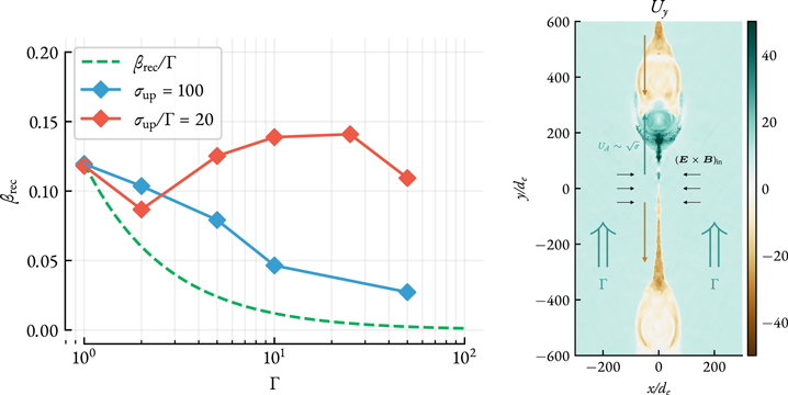
Figure 11. Left: reconnection rate, measured as βrec = ( E × B )in/B2 in the upstream for localized 2D simulations initialized with an upstream flying with a Lorentz factor of Γ along the current layer. The green dashed line shows the naive expectation that the rate, being universal in the proper frame of the upstream plasma, in the lab frame should scale as 1/Γ. Right: zoom in of a region of our simulation with σup = 100, Γ = 10. The plot shows the four-velocity component of plasma along the sheet, Uy . Initially, the upstream plasma is pushed in the +y-direction. In the current sheet, nevertheless, relativistic outflows move in both directions, where the x-points in-between are static.
Download figure:
Standard image High-resolution imageTo understand this effect, let us consider separately the velocities of relativistic outflows from the x-point (as shown in the right panel of Figure 11). In the frame co-moving with the upstream plasma, the velocities of these outflows should be symmetric w.r.t. the y-axis. Or in other words, , where dashed quantities are measured in the frame co-moving with upstream plasma. Here "±" indicate the direction of motion along and opposite to the current layer (the y-axis). Boosting back to the lab frame we find: , and , assuming the "upstream" frame moves along the y-axis with a Lorentz factor of Γ ≫ 1. Cold upstream magnetization (not including bulk Lorentz factor) in the lab frame, σ ≡ B2/(4π ρe c2), can be expressed as , since Bup = By does not transform, and . Then the outflow velocities in the lab frame can be written as: , and , where is the relativistic Alfvén velocity in the lab frame. This can be also seen in the right panel of Figure 11: outflow velocities along the y-axis measured in the lab frame are clearly asymmetric. When Γ1/2 becomes comparable to , the outflow velocity in the direction opposite to the upstream boost, u−, may become nonrelativistic. In this case, it is natural to expect the reconnection rate, defined in our case as βrec ≡ vin/vout ≈ vin/c to drop, since the effective outflow three-velocity, vout, can now be smaller than c.


Arguments provided in this section are not exhaustive, and should rather be taken as possible explanations of empirical facts, observed in numerous simulations. Further investigation is definitely necessary to better understand the nature of the mechanism that controls the reconnection rate in these cases.
Appendix D: Energy Distribution of Particles in the Different Parts of the Simulation Domain
For the simulation R75_ang0, the magnetization parameter in the upstream, shown in Figure 6, is close to σLC ∼ 103 (as shown with the line-out plot on the right) and drops to zero inside the current sheet, where the magnetic field vanishes. This means that the characteristic energies to which particles can get accelerated in the current sheet are comparable to σ me c2 (as will be demonstrated shortly).
Let us consider distribution functions for e± in different regions of our simulation R75_ang0, as shown in Figure 12. On a poloidal slice in Figure 12(a), we show the bulk Lorentz factor of the plasma, , which is computed using the bulk four-velocity, U = ∫ u f( u )d3 r . Figures 12(b), 12(c), and 12(d) show the distribution functions of the electrons and positrons in three different regions: in the separatrix (last closed field line), in the current sheet, and in the upstream correspondingly. Upstream plasma is relatively cold; electrons and positrons flow outwards along the magnetic field lines, gaining characteristic bulk Lorentz factors of Γ ∼ 10 (Figure 12(d)). On the separatrix (Figure 12(b)), both electrons and positrons from the surface are marginally accelerated by an unscreened electric field, gaining energies close to 〈γ〉 ∼ 10–100. This region also hosts hot electrons returning from the Y-point, which is evident from the excess of electrons at Lorentz factors of a few 102 shown in Figure 12(b).


Figure 12. Distribution functions of electrons and positrons measured in different locations of our simulation shown on an azimuthally averaged poloidal slice. Synchrotron cooling in this particular simulation (R75_ang0_gr2) is weak. The bulk Lorentz factor is shown in panel (a). Panels (b), (c), and (d) show distribution functions in the separatrix, the current layer, and the upstream, respectively. Plasma in the upstream is typically cold with a bulk outflow Lorentz factor of a few. In the current sheet, the bulk motion of plasma is dictated by the dynamics of reconnection, and the characteristic outflow velocities are comparable to the Alfvén speed with a Lorentz factor . As expected, the highest-energy particles are produced in the current layer where magnetic reconnection occurs.

Download figure:
Standard image High-resolution imageThese two regions, the upstream and the separatrix, act as an "intake" and an "exhaust" for the current sheet. It is important to note that particles in these regions are generally exposed to a substantial orthogonal magnetic field component. This means that high-energy particles from the current sheet cannot exist there for timescales longer than the short cooling time. Thus, the main role in shaping the observed γ-ray emission is played by the current sheet, where constant release of magnetic energy sustainably accelerates particles in x-lines, where the magnetic field strength is zero (the cooling is nonexistent).
In the current sheet (Figure 12(c)) we see a substantial nonthermal particle population, extending to γ ∼ σ ∼ 500–1000. The bulk motion of the current sheet, on the other hand, has a Lorentz factor of Γ ∼ 10–100, consistent with characteristic velocities of relativistic flows along the current sheet during the reconnection, (which corresponds to the Alfvén speed). 24 Notice, also, that the distributions of electrons and positrons are slightly different: positrons extend to slightly higher energies. This is due to the fact that the electric field generated during reconnection "pushes" the electrons opposite to the global E × B drift, which is charge-invariant and directed radially outward (in Figure 3(a), the reconnection electric field is pointing in the out-of-plane direction and has both toroidal and radial components). This difference in the electrons and positrons has been observed in earlier simulations (see, e.g., Cerutti et al. 2015); however, it almost vanishes for large obliquity angles, χ, which we also see in our simulations.

Footnotes
- 6
This number varies from around ∼1000 in the small region near the surface of the star to a few-to-ten in the bulk of the magnetosphere, and ∼100 in the current layer.
- 7
It is important to mention that our technique of providing the magnetosphere with fresh plasma is different from the more self-consistent methods used in previous works (Chen & Beloborodov 2014; Philippov et al. 2015). To simplify the simulation as well as to reduce the number of input parameters, we do not model the full pair-production process. However, as was demonstrated in earlier works (Belyaev 2015; Cerutti et al. 2015), the structure of the outer magnetosphere is unaffected by the pair injection prescription near the polar cap.
- 8
More details on how the coupled particle pusher algorithm works can be found in Appendix B.
- 9
Simulations with the same basic parameters and other obliquity angles are, correspondingly, R75_ang20, R75_ang60, and R75_ang90.
- 10
In addition to the motion along the field lines, particles also experience an E × B drift. However, the Lorentz factor associated with the drift is rather small within a few light cylinders from the star.
- 11
Notice that the exact value of δcs is irrelevant, since (for θ ∈ (π/2 − δcs/r, π/2 + δcs/r)), as long as δcs ≪ r.
- 12
In fact, in the radiative regime considered in our simulations, a considerable amount (about half) of the dissipated energy is radiated away, with the other half being deposited into the acceleration of pairs.
- 13
More details of our findings together with some discussion can be found in the Appendix C.
- 14
We see this at resolution of , where . For the higher resolution of (2200x)3 considered, e.g., in Figure 4, and , we see no signs of this effect.
- 15
In terms of PIC simulations, defining dimensionless γrad is equivalent to upscaling the classical electron radius, re , to boost the relative efficiency of synchrotron losses. Also note that in this rough definition, the magnetic field is considered to be exactly perpendicular to the motion of a particle. In our simulations, as well as in reality, particles flying at small pitch angles w.r.t. the magnetic field will be cooled less efficiently. Thus, γrad can be thought of as just a proxy for the average cooling efficiency for a population of isotropically distributed particles.
- 16
For computational purposes, we limit injection only to field lines close to the equator that participate in reconnection. Since particles are well magnetized and any transport in the transverse direction to the magnetic field is suppressed, the field lines at higher altitudes have little to no effect on the reconnection process.
- 17
The growth rate of the instability is defined as c/wcs in the rest frame of the upstream plasma and should be Lorentz-boosted appropriately.
- 18
Here and further in this section we normalize all of the quantities to fiducial values of erg s−1), , and (plasma multiplicity w.r.t. the local Goldreich–Julian value). For reference, varies between 1032 and 1038 erg s−1 (Vela: 7 × 1036 erg s−1, Crab: 4 × 1038 erg s−1), B* weakly changes between 1012 − 1013 G, and κ ≈ 102–107 (where ≳104 is the case only for a few of the youngest pulsars, e.g., the Crab). In practice, κ is determined by the dynamics of the polar cap discharge, and the pair-production efficiency near the light cylinder, both of which indirectly depend on and B* (or P and ). But for the purposes of this discussion, we omit this dependency.
- 19
The value of Γ, which is the Lorentz factor of the bulk motion of pairs flowing from the polar cap to the outer magnetosphere, is set by the last curvature photons to pair produce before escaping the polar cap discharge region. The energy of pairs produced by these photons is determined by the angle, ψ, between the photon momentum and the magnetic field: γ± ≈ 1/ψ (this is valid in the limit where the energies of photons are large: ≫me c2, and the angle ψ ≪ 1; see, e.g., Timokhin 2010). Since the discharge operates up to ≈R* from the surface of the star, the last photons to pair produce will have ψ ≈ R*/Rc , where Rc is the radius of curvature of the magnetic field lines . From these, we finally find: .
- 20
See also similar arguments in the context of the M87* by Ripperda et al. (2022).
- 21
For the least energetic γ-ray-emitting pulsars with erg s−1, it is likely that the polar cap discharge is less efficient, and the resulting plasma multiplicity near the light cylinder is κ ≲ 103, which yields the same cutoff energy.
- 22
Notice that the total multiplicity κ = κLC + κPC, where κPC is the multiplicity of the pair cascade near the polar cap.
- 23
This means that gyration of the coldest particles is extremely underresolved near the surface of the star. This is only possible because of the coupled GCA/Boris particle pusher we employ.
- 24
The slight enhancement is due to the fact that there is a bulk E × B outflow of the current sheet, similar to the wind in the upstream.


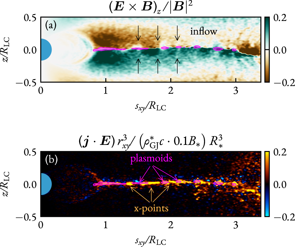
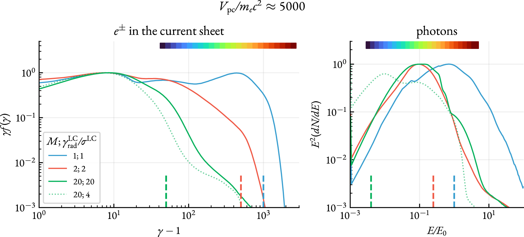