


Abstract
Planet formation by pebble accretion requires an efficient inward flux of icy pebbles to explain the many mini-Neptunes and super-Earths discovered by Kepler within 1 au. Recently, hints of large-scale pebble migration have been found in the anticorrelation between the line ratio of water-to-other volatiles detected in medium-resolution (R ∼ 700) Spitzer/IRS spectra and the dust disk radius measured at millimeter wavelengths with the Atacama Large Millimeter Array. Here, we select three disks in Taurus that span the range of measured line flux ratios (a factor of ∼5) and dust disk radii (1 order of magnitude) and model their Spitzer/IRS spectra assuming gas in local thermodynamic equilibrium to retrieve the water column density in their inner disks. We find that, at the Spitzer/IRS resolution and sensitivity, large uncertainties in the retrieved column densities preclude resolving the expected difference of a factor of ∼5 in water abundance. Next, we simulate higher-resolution (∼3000) JWST/MIRI spectra at the signal-to-noise ratio of ∼100, which will be obtained via the Guaranteed Time and General Observation programs and apply the same retrieval approach used with Spitzer/IRS spectra. We show that the improved resolution and sensitivity of JWST/MIRI significantly reduce the uncertainties in the retrieved water column densities and will enable quantifying the difference in the inner water column of small versus large dust disks.
Export citation and abstract BibTeX RIS

Original content from this work may be used under the terms of the Creative Commons Attribution 4.0 licence. Any further distribution of this work must maintain attribution to the author(s) and the title of the work, journal citation and DOI.
1. Introduction
In recent years, there has been an exponential growth in the number of exoplanets detected around other stars, mostly due to dedicated space missions like Kepler and its successor, TESS (e.g., Borucki 2018). At the same time, state-of-the-art ground-based facilities such as the Atacama Large Millimeter Array (ALMA) have enabled surveys and in-depth studies of disks around young stars (e.g., Andrews 2020). Therefore, we are currently in a position where we can learn about planet formation from both the demographics of formed exoplanets and their birth environments.
During its mission, Kepler revealed that planets with radii between Earth and Neptune are the most common, with an occurrence rate greater than 60% within 200 days (Mulders et al. 2019). Of these planets, those with radii larger than 2 R⊕ have low densities consistent with H/He envelopes greater than 1% of the total mass, see, e.g., Figure 3 in Hadden & Lithwick 2017). These findings suggest that many of the close-in mini-Neptunes/super-Earths formed in the protoplanetary disk phase and have prompted the development of new planet formation models where efficient growth occurs by the accretion of millimeter-to-centimeter-sized dust grains, also called pebbles (e.g., Johansen & Lambrechts 2017). Because most of the mass in disks is located at large radial distances, a critical parameter in these so-called pebble-accretion models is the inward influx of icy pebbles. For instance, models by Lambrechts et al. (2019) require a substantial integrated pebble flux ≳200 M⊕ over 1 million yr within 1 au to form mini-Neptunes/super-Earths. Is there observational evidence for icy pebbles drifting inward as close in as 1 au?
Millimeter observations are sensitive to pebbles at tens of astronomical units in disks around young stars. ALMA surveys of entire star-forming regions carried out at moderate spatial resolution and sensitivity have provided statistics on the amount of pebbles and their outermost radial location (e.g., Ansdell et al. 2016; Barenfeld et al. 2016; Hendler et al. 2020; Pascucci et al. 2016). In parallel, dedicated high-resolution ALMA observations of selected disks have shown that dust substructures are prevalent in large disks (e.g., Andrews et al. 2018) while compact disks appear smooth (Long et al. 2019). The observed larger gas than dust disk radii (e.g., Sanchis et al. 2021) suggests that pebbles have drifted inward and smaller dust disks may have experienced more efficient radial drift in the absence of disk substructures (e.g., Facchini et al. 2019; Trapman et al. 2019).
The radial drift and evaporation of icy pebbles can lead to significant enhancements of gas-phase abundances inside the snowlines of major volatiles species (e.g., Cuzzi & Zahnle 2004). For the highly volatile CO molecule, inferred radial abundance profiles (Zhang et al. 2019) show similarities to models of pebble drift and evaporation (Krijt et al. 2018; Stammler et al. 2017), and can in some cases be used to constrain the pebble flux at the CO snowline location (Zhang et al. 2020)—typically between 10 and 100 au.
Understanding whether icy pebbles from the outer disk drift as close in as 1 au require combining ALMA data with infrared (IR) spectroscopic observations. The wavelength range covered by moderate-resolution (R ∼ 700) Spitzer/IR spectra is particularly useful as it probes volatiles in the disk surface, including water vapor, within the water snowline (e.g., Pontoppidan et al. 2014). Therefore, Spitzer/IRS spectra can indirectly trace those icy pebbles that drifted inside a few astronomical units, and released water vapor upon crossing the snowline. A study by Banzatti et al. (2020) found that the ratio of H2O emission lines at ∼17 μm with respect to rovibrational lines from three other volatiles (HCN, C2H2, and CO2) is anticorrelated with the dust disk radius inferred from ALMA observations, i.e., with the outermost location of pebbles. A modest anticorrelation is also present between the H2O luminosity, normalized by accretion luminosity, and the dust disk radius. These anticorrelations hint that small disks have a higher water vapor content inside the snowline and have been interpreted in the context of inward drift of icy pebbles, i.e., disks with small dust radii have experienced more inward drift of icy pebbles, which then released water vapor into the inner disk.
Follow-up theoretical work by Kalyaan et al. (2021) investigated how the appearance of gaps and the associated gas pressure maxima reduce the inward drift of pebbles and water delivery to the inner disk. They find that disks without gaps experience significantly more water enrichment in their inner regions than disks with gaps. Depending on the pebble size and several other parameters, variations in the (peak) inner disk water abundance can exceed a factor of 10. Their grid of models identifies the 7–15 au region as the sweet spot for a gap to efficiently block the inward pebble migration to the inner disk and they argue that such disks are unlikely to form super-Earths.
This work takes the study of Banzatti et al. (2020) one step further as it asks whether the broad range of measured H2O/HCN flux ratios can be attributed to different column densities of water vapor. In Section 2, we select three representative disks that span a factor of 5 in their H2O/HCN flux ratio, thus covering the measured range. Section 3 details our modeling strategy, which builds on the the Continuum and Line fItting Kit (CLIcK; Liu et al. 2019) to model the entire water emission covered in the Spitzer/IR spectra. In Section 4, we simulate water emission spectra at the enhanced spectral resolution of JWST/MIRI and show that sensitive JWST exposures can discriminate between disks that differ by a factor of 5 in their water column density. A summary of our findings and further discussion can be found in Section 5.
2. Sample Selection and Main Properties
Our goal is to test whether the H2O/HCN flux ratio versus dust disk radius relation is driven by the water abundance in the inner disk as proposed in Banzatti et al. (2020). As such, we have chosen two disks from Banzatti et al. (2020) that cover the extremes of the relation (DK Tau A and IQ Tau), as well as a disk that falls in the middle (BP Tau), see Figure 1. DK Tau has a small dust disk of only 15 au while IQ Tau has the largest dust disk (Rdust ∼ 160 au). In the context of efficient inward drift of pebbles, these radii are mostly set by the outermost gas pressure bump (e.g., Pinilla et al. 2020).

Figure 1. H2O/HCN flux ratio vs. dust disk radius and best-fit relation (dashed line) from Banzatti et al. (2020). Our selected sources are highlighted: DK Tau A and IQ Tau cover the extremes of the relation while BP Tau is in the middle.
Download figure:
Standard image High-resolution imageBP Tau and IQ Tau are single stars while DK Tau A has a relatively wide companion at ∼2 4 (∼300 au) that falls within the Spitzer/IRS slit but contributes <10% to the broadband mid-infrared flux (McCabe et al. 2006), and because it is a lower mass star than DK Tau A, likely even less to the water and HCN emission (Pascucci et al. 2013). We also note that the dust disk of DK Tau A is unlikely to have been truncated by the companion as it would require it to be on a very eccentric (e > 0.7) orbit (Manara et al. 2019).
8
We preferred disks from the same star-forming region, hence similar age, and selected Taurus because of the recent high-resolution ALMA survey providing accurate dust disk radii (hereafter Rdust, Long et al. 2019). As line fluxes scale with the source distance, we also selected disks at the same distance within the typical Gaia uncertainty of ∼2 pc. Finally, we made sure that our selected stars have a similar spectral type (SpTy) as the detection rate and that the strength of the water lines is spectral-type dependent (Pascucci et al. 2013; Pontoppidan et al. 2010).
4 (∼300 au) that falls within the Spitzer/IRS slit but contributes <10% to the broadband mid-infrared flux (McCabe et al. 2006), and because it is a lower mass star than DK Tau A, likely even less to the water and HCN emission (Pascucci et al. 2013). We also note that the dust disk of DK Tau A is unlikely to have been truncated by the companion as it would require it to be on a very eccentric (e > 0.7) orbit (Manara et al. 2019).
8
We preferred disks from the same star-forming region, hence similar age, and selected Taurus because of the recent high-resolution ALMA survey providing accurate dust disk radii (hereafter Rdust, Long et al. 2019). As line fluxes scale with the source distance, we also selected disks at the same distance within the typical Gaia uncertainty of ∼2 pc. Finally, we made sure that our selected stars have a similar spectral type (SpTy) as the detection rate and that the strength of the water lines is spectral-type dependent (Pascucci et al. 2013; Pontoppidan et al. 2010).
Relevant stellar and disk parameters for our sample are summarized in Table 1. In addition to the parameters discussed above, we also collect stellar bolometric luminosities (L*), stellar masses (M*), X-ray luminosities (LX
), and accretion luminosities (Lacc). The latter two quantities are included here because thermo-chemical models show that they affect the abundance of volatiles in disk atmospheres as well as their luminosity (e.g., Greenwood et al. 2019; Najita et al. 2011). For instance, Najita et al. (2011) find that the warm column of C2H2 drops by a factor of 2 when LX
is increased from 1029 to 1030 erg s−1, while the warm column of the other molecules investigated in Banzatti et al. (2020) remains essentially the same. Greenwood et al. (2019) further illustrate the sensitivity of H2O to the accretion luminosity: when the UV excess flux is increased by a factor of 20 (from 10−3 to 2 × 10⁻²
L⊙) the 17.75 μm line flux of water increases by a factor of ∼3. Observations suggest a much stronger dependence between the line luminosity of water, as well as the other molecules discussed above, and accretion luminosity of the form  (e.g., Banzatti et al. 2020).
Table 1. System Properties
| Source | D | SpTy | L* | M* | logLX | Lacc | Rdust | Incl. |
|---|---|---|---|---|---|---|---|---|
| (pc) | (L⊙) | (M⊙) | (L⊙) | (L⊙) | (au) | (deg) | ||
| DK Tau A | 128 | K8.5 | 0.45 | 0.6 | −3.7 a | 0.14 | 15 | 12.8 |
| BP Tau | 129 | M0.5 | 0.40 | 0.5 | −3.5 | 0.15 | 41 | 38.2 |
| IQ Tau | 131 | M1.1 | 0.22 | 0.5 | −4.0 | 0.11 | 159 | 62.1 |
Notes. The source distance (D), SpTy, L*, M*, Rdust, and disk inclination (incl.) are from Long et al. (2019). LX are from Table 5 of Güdel et al. (2007) while Lacc are from Table 1 of Hartmann et al. (1998), scaled here to the Gaia distances.
a This is the combined AB X-ray luminosity, see Güdel et al. (2007).Download table as: ASCIITypeset image
Stellar luminosities and masses are from Long et al. (2019) and have typical uncertainties of ∼20% (Herczeg & Hillenbrand 2014; Pascucci et al. 2016). Given these uncertainties, the three sources have essentially the same stellar masses and only IQ Tau differs in bolometric luminosity from the other two by being a factor of ∼2 fainter. Stellar X-ray luminosities are from Table 5 of Güdel et al. (2007), rescaled to the Gaia distances in Table 1. Among the three sources, BP Tau is the strongest X-ray emitter, followed by DK Tau A + B, which is at least 40% fainter. The X-ray luminosity of IQ Tau has a large uncertainty, within 1σ its LX is the same as that of the DK Tau binary but could also be a factor of ∼2 fainter. Finally, the accretion luminosities reported in Table 1 are taken from Table 1 in Hartmann et al. (1998), with the methodology developed in Gullbring et al. (1998), and are based on the most reliable accretion diagnostic, which is the UV excess from the accretion shock on the stellar surface. The difference in the estimated Lacc is less than 50%, well within the quoted typical uncertainty of a factor of ∼3, which means that the three sources are essentially indistinguishable in their accretion luminosity. For completeness, we point out that DK Tau A and BP Tau also have more recent Lacc estimates based on high-resolution Keck spectra taken in 2008 and using several permitted emission lines, which are considered secondary/less reliable accretion diagnostics. The estimated Lacc for DK Tau A is ∼0.16 L⊙, essentially the same as the one inferred from the UV excess, while the one for BP Tau is a factor of ∼2.5 lower (Fang et al. 2018) but still within the typical accretion luminosity uncertainty. Interestingly, their water luminosity (Banzatti et al. 2020) over  covers 1 order of magnitude as their inferred dust disk radii. The evolutionary tracks of vapor enrichment versus dust disk radius in Figure 10 of Kalyaan et al. (2021), predict that the mass in water vapor in the inner disk of DK Tau should then be ∼5 times that of the inner disk of IQ Tau. This factor of ∼5 enrichment is essentially the same as the one inferred from the H2O/HCN flux ratio.
In addition to differences in disk radii and H2O/HCN flux ratios, which were chosen to span the extreme and middle points of the relation shown in Figure 1, IQ Tau has a significantly more inclined disk than DK Tau A and BP Tau. This might contribute to an overall fainter IR continuum emission and weaker lines, see Figure 2. Another major difference is in the continuum flux density of DK Tau and BP Tau, the former being twice as large as the latter, 9 in spite of the two sources being essentially at the same distance and having a very similar stellar luminosity, but see Appendix A for a possible caveat on the stellar luminosity of DK Tau A reported in Long et al. (2019). As we elaborate in Appendix A, different disk parameters are most likely the source of the different infrared continua.
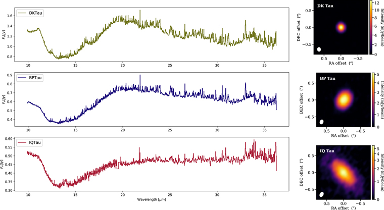
Figure 2. Spitzer/IRS spectra probing water vapor in the inner disk (Pontoppidan et al. 2010) next to ALMA high-resolution images tracing the outer dust disk emission (Long et al. 2019). Note that the IRS spectrum of DK Tau includes emission from the disks around the A and B components but B contributes < 10% to the broadband mid-infrared flux (McCabe et al. 2006).
Download figure:
Standard image High-resolution image3. Modeling of the Spitzer/IRS Spectra
The Spitzer/IRS spectra we have modeled as part of this investigation are those published in Pontoppidan et al. (2010) and downloadable via the main author's website. 10 These spectra have an average resolution of R ∼ 700 and include both the Short High (SH, ∼10–19 μm) and Long High (LH, ∼20–35 μm) modules. As we noted a jump of ∼10% between the SH and LH modules in IQ Tau, we shifted down the LH to match the SH in this spectrum. The spectra used for the modeling, next to the ALMA continuum images tracing the outer disk radius, are shown in Figure 2.
3.1. Prior Modeling
Carr & Najita (2011) independently reduced the SH portion of the DK Tau and BP Tau IRS spectra. After subtracting the continuum emission, which is identified by fitting polynomials to six to eight separate wavelength regions, they focused on modeling the water emission in the 12–16 μm portion of the SH spectra. Their model assumes a plane parallel slab of gas in local thermodynamic equilibrium (LTE) and has three main parameters: a single gas temperature (T), column density ( ), and emitting radius (Re
). Synthetic water spectra were calculated over a range of temperatures and column densities and compared to the observed spectra to identify, by visual inspection, the best fit. For each combination of temperature and column density, the emitting radius was then adjusted to match the observed line fluxes. Using this approach, they find the same gas temperature (650 K), and within their 1σ uncertainty, the same column density (∼7 × 1017 cm−2) for DK Tau and BP Tau. Thus, the brighter water emission in DK Tau is interpreted as due to a larger emitting radius, 1.3 au versus 0.8 au for DK Tau and BP Tau, respectively.
), and emitting radius (Re
). Synthetic water spectra were calculated over a range of temperatures and column densities and compared to the observed spectra to identify, by visual inspection, the best fit. For each combination of temperature and column density, the emitting radius was then adjusted to match the observed line fluxes. Using this approach, they find the same gas temperature (650 K), and within their 1σ uncertainty, the same column density (∼7 × 1017 cm−2) for DK Tau and BP Tau. Thus, the brighter water emission in DK Tau is interpreted as due to a larger emitting radius, 1.3 au versus 0.8 au for DK Tau and BP Tau, respectively.
The third source in our sample, IQ Tau has been modeled by Salyk et al. (2011) assuming the same isothermal slab approximation as in Carr & Najita (2011) but using the spectra from Pontoppidan et al. (2010) and a different approach for the continuum subtraction. Specifically, Salyk et al. (2011) identified 65 water lines from the combined SH and LH modules (10–35 μm) and performed a local continuum subtraction around each line. From a grid of models with varying temperature and column density, they then find the values that minimize the difference between the 65 observed and modeled line peaks, using the emitting area as a scaling factor. Through this approach, they derive a hot surface of 800 K for IQ Tau,  cm−2, and a small Re
of ∼0.5 au. Unfortunately, neither DK Tau nor BP Tau are included in this paper.
cm−2, and a small Re
of ∼0.5 au. Unfortunately, neither DK Tau nor BP Tau are included in this paper.
As a comparison of both techniques, we summarize here the results for the disk of AA Tau which is modeled both by Carr & Najita (2011) and by Salyk et al. (2011). For this disk, both papers report the same water-emitting radii within the quoted uncertainties: 0.85 ± 0.12 and 0.74 au, respectively. However, Carr & Najita (2011) obtain a temperature of 575 K and  cm−2 while Salyk et al. (2011) report a cooler temperature of 400 K and a column density of water that is almost 1 order of magnitude higher, 6.3 × 1018 cm−2. This comparison highlights the known degeneracy between temperature and column density, with decreasing T offset by increasing
  (e.g., Carr & Najita 2011), and illustrates that results depend heavily on what technique is used, see also discussion in the PPVI chapter by Pontoppidan et al. (2014). It also points to the need for consistent modeling of the three sources to test the hypothesis that their location in the H2O/HCN flux ratio versus dust radius plot is driven by the water abundance in the inner disk.
3.2. Our Modeling Approach with CLIcK
This work utilizes an adapted version of CLIcK developed by Liu et al. (2019). In its original version CLIcK simultaneously fits the dust continuum emission, assuming a simple two-layer disk model, and gas lines, assuming a slab of gas in LTE at constant or radially varying temperature. The code is built upon the single temperature LTE slab of Pascucci et al. (2013). which has been tested against the one developed in Banzatti et al. (2012). The code has been also tested on the Spitzer/IRS spectrum of AA Tau reduced and shared by J. Carr, and within the quoted uncertainties, finds the same T,  ,
11
and Re
as Carr & Najita 2011 when fitting the same 12–16 μm portion of the SH spectrum. As expected, when extending the fit to the LH, the gas temperature inferred by CLIcK diminishes, and for the case of a radially decreasing power-law profile, its value at 1 au is consistent with that reported in Salyk et al. (2011). However, the emitting radius remains greater than 1 au, which means that the inferred water column density increases only slightly and stays a factor of ∼6 lower than that given in Salyk et al. (2011), still consistent with the value and uncertainty in Carr & Najita (2011). Furthermore, Liu et al. (2019) generated a reference disk model using RADMC for the continuum and RADLite for lines and demonstrated that CLIcK can retrieve the properties of the water-emitting region.
,
11
and Re
as Carr & Najita 2011 when fitting the same 12–16 μm portion of the SH spectrum. As expected, when extending the fit to the LH, the gas temperature inferred by CLIcK diminishes, and for the case of a radially decreasing power-law profile, its value at 1 au is consistent with that reported in Salyk et al. (2011). However, the emitting radius remains greater than 1 au, which means that the inferred water column density increases only slightly and stays a factor of ∼6 lower than that given in Salyk et al. (2011), still consistent with the value and uncertainty in Carr & Najita (2011). Furthermore, Liu et al. (2019) generated a reference disk model using RADMC for the continuum and RADLite for lines and demonstrated that CLIcK can retrieve the properties of the water-emitting region.
For our selected disks, we first experimented extensively with the stellar and disk input parameters to simultaneously fit the continuum and line emission. However, due to the different and complex mixture of dust grains that are present in these spectra (see Sargent et al. 2009 and Appendix A), we could not find any satisfactory fit. As such, we modified CLIcK to (i) generate a continuum through interpolation at wavelengths deemed to be free of line emission; (ii) subtract such continuum from the spectrum; and (iii) fit the continuum-free spectrum with a slab of gas in LTE. Figure 3 shows the continuum-subtracted spectra and highlights in light blue the wavelength regions used in CLIcK to fit the water emission. Note that, at the Spitzer resolution, water lines are often a blend of multiple transitions (e.g., Pontoppidan et al. 2010 and Table 5 in Appendix C for a few examples), which leads to significant model fit degeneracies (e.g., Pontoppidan et al. 2014 and Sections 3.1 and 4). Transitions attributed to other atoms and molecules, hence excluded from the fit, are also marked. In these continuum-subtracted spectra, the peak flux density of the water lines decreases going from DK Tau, which has the smallest dust disk, to BP Tau, the intermediate-size disk, to IQ Tau, which has the largest dust disk in our sample.
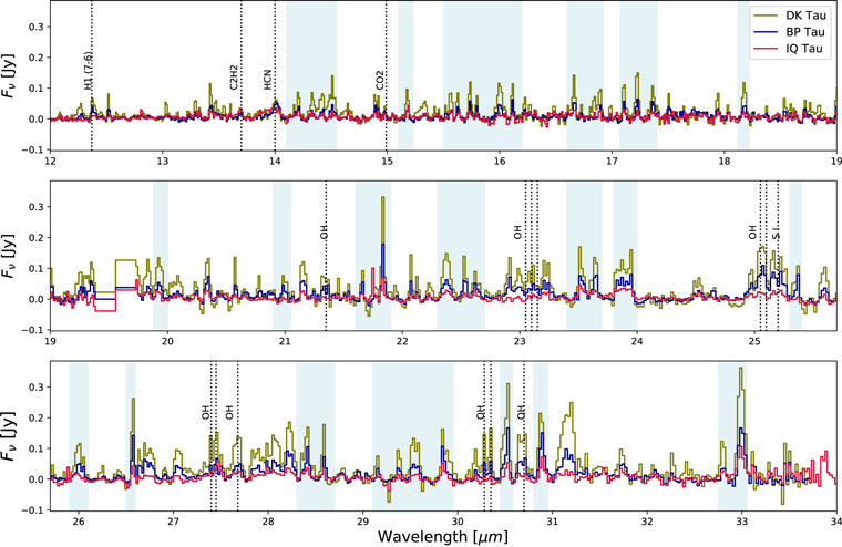
Figure 3. Continuum-subtracted spectra for DK Tau, BP Tau, and IQ Tau. The light blue shaded regions (hereafter referred to as selected-λ region) include strong water emission uncontaminated by other known atomic or molecular line, and as such, are selected to fit the water spectrum (see Section 3).
Download figure:
Standard image High-resolution imageNext, we run a grid of models to fit the water emission in the continuum-subtracted spectra. CLIcK assumes that gas is in LTE but the temperature can vary radially; more specifically, it can decrease with a power-law dependence on the radial distance from the star. We use this option of decreasing gas temperature as it has been shown that it can better fit the entire water spectrum covered by Spitzer/IRS (Liu et al. 2019). In this option, the temperature is defined via two parameters: its value at 1 au (T1au) and the power-law index p where  . As in previous modeling efforts (see Section 3.1), the other two input parameters in our model are the radius of the emitting area (Re
) and the water column density in the emitting region (
. As in previous modeling efforts (see Section 3.1), the other two input parameters in our model are the radius of the emitting area (Re
) and the water column density in the emitting region ( ). After running models with these four varying input parameters on the water-rich spectra of DK Tau and BP Tau, we found that the distribution of power-law indices narrowly peaked at 0.5. Hence, to better constrain the other three parameters for the water-faint source IQ Tau, we opted to fix p to 0.5 in all subsequent runs.
The grid of models we present here consists of 40 different values for  and Re
, and 36 different values for T1au resulting in 57,600 models per source. The grid spacing for
and Re
, and 36 different values for T1au resulting in 57,600 models per source. The grid spacing for  is logarithmic while the grid spacing for Re
and T1au is linear. Thanks to the density of these grids, we could skip the optional Markov Chain Monte Carlo refinement within CLIcK and identify the best-fit model, i.e., the one with the lowest χ2. To estimate the uncertainty of the best-fit parameter set, we carried out a Bayesian analysis assuming flat priors as we have no preliminary information about the parameters. The relative probability of a model in the parameter space is given by
is logarithmic while the grid spacing for Re
and T1au is linear. Thanks to the density of these grids, we could skip the optional Markov Chain Monte Carlo refinement within CLIcK and identify the best-fit model, i.e., the one with the lowest χ2. To estimate the uncertainty of the best-fit parameter set, we carried out a Bayesian analysis assuming flat priors as we have no preliminary information about the parameters. The relative probability of a model in the parameter space is given by  (e.g., Lay et al. 1997; Pinte et al. 2008). Then, the marginalized probability distribution for each parameter
  is obtained by first adding the individual probabilities of all the models with a common value of the parameter θ and then normalizing to the total probability for that parameter. For instance, the probability for the temperature T is
where n is the number of models that contain the value Ti . Examples of marginalized probabilities are provided in, e.g., Figure 3 of Liu et al. (2019), and discussed later for our fits. From these curves, 1σ uncertainties are calculated as the ranges that include 68% of the area. In relation to the example above

with ζ = 0.68 and T−1σ and T+1σ being the 1σ uncertainties on the temperature.
3.2.1. Large Uncertainties in Water Columns Preclude Resolving the Expected Difference in Abundance
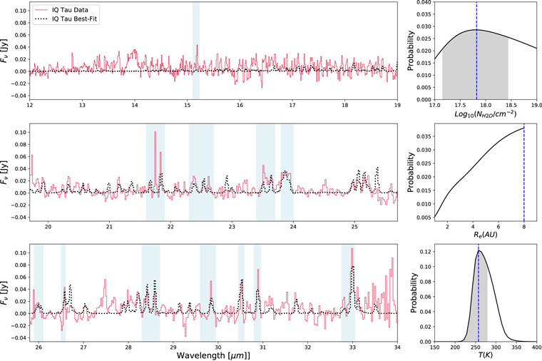
The best-fit model for DK Tau is presented in Figure 4 while those for BP Tau and IQ Tau are provided in Appendix B, see Figures 9 and 10. In these figures, the best-fit model is shown with a black dotted line on top of the continuum-subtracted spectrum (solid colored line). The three rightmost panels provide the Bayesian probability distributions  for the water column density (
 ), emitting radius (Re
), and temperature (T) with the best-fit value indicated by a blue vertical dashed line. The shaded gray region gives the 68% area used to calculate the 1σ confidence intervals for each input parameter. These best-fit values and 1σ uncertainties are also summarized in Table 2.
), emitting radius (Re
), and temperature (T) with the best-fit value indicated by a blue vertical dashed line. The shaded gray region gives the 68% area used to calculate the 1σ confidence intervals for each input parameter. These best-fit values and 1σ uncertainties are also summarized in Table 2.
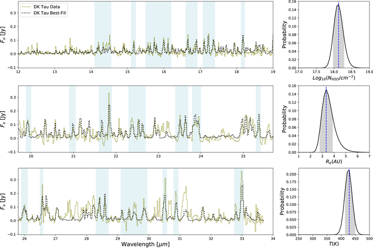
Figure 4. Left panels: best-fit model (black dotted line) superimposed on the continuum-subtracted spectrum of DK Tau (colored line). The light blue shaded regions are those that contribute to the χ2 calculation in fitting the water spectrum. Right panels: Bayesian probability distributions for the column density (top), emitting radius (middle), and gas temperature (bottom) with the best-fit parameters as blue dashed lines and the 68% confidence intervals as gray-shaded regions.
Download figure:
Standard image High-resolution imageTable 2. Best-fit Parameters and Uncertainties
| Source |

| Re | T1au | χ2 |
|---|---|---|---|---|
| (cm−2) | (au) | (K) | ||
| DK Tau A |

|

|

| 418 |
| BP Tau |

|

|

| 100 |
| IQ Tau |

| ⋯ |

| 30 |
Note. The water emitting radius for IQ Tau is unconstrained. Note that χ2 is not the reduced value and the lower number for IQ Tau is driven by the smaller portion of spectrum used in the fit, see Figure 10.
Download table as: ASCIITypeset image
We find that the emitting radii for DK Tau and BP Tau are the same within the quoted 1σ uncertainties while Re
remains unconstrained for IQ Tau. Gas temperatures at 1 au are different, even when considering 1σ uncertainties, and we note that the fainter the water emission the cooler the inferred gas temperature. On the water column density, which is the most interesting parameter for this study, only DK Tau has, at face value, a larger column density than the other two sources by a factor of ∼2. This is the same factor as the H2O/HCN flux ratio of DK Tau to BP Tau. However, the uncertainties in  are such that all inferred water column densities are consistent with each other within 1σ. If the H2O/HCN flux ratio scales linearly with
  we should have found a ∼5 times lower column density for IQ Tau than for DK Tau. However, there are so few faint lines detected in the continuum-subtracted spectrum of IQ Tau that, not only Re
is unconstrained, but also the
we should have found a ∼5 times lower column density for IQ Tau than for DK Tau. However, there are so few faint lines detected in the continuum-subtracted spectrum of IQ Tau that, not only Re
is unconstrained, but also the  uncertainty remains very large. If we fix Re
to 3 au, the same emitting radius for DK Tau and BP Tau, and consider gas at 300 K (slightly warmer than the best fit but within the 1σ uncertainty), we obtain
uncertainty remains very large. If we fix Re
to 3 au, the same emitting radius for DK Tau and BP Tau, and consider gas at 300 K (slightly warmer than the best fit but within the 1σ uncertainty), we obtain  . This is a factor of ∼5 from the value for DK Tau and with the more constrained value on the 1σ uncertainty puts the column density for IQ Tau below both DK and BP Tau. Besides the degeneracy between T and
  mentioned in Section 3.1, this modeling effort shows that uncertainties in the retrieved gas parameters need to be reduced to test if the H2O/HCN flux ratio versus dust disk radius relation is truly driven by the water abundance in the inner disk. As we show in the next section this can be achieved with JWST/MIRI.
4. JWST/MIRI Simulated Spectra
As available Spitzer/IRS spectra are insufficient to detect differences in water column densities, here we explore the capabilities of JWST/MIRI. To this end, we compute synthetic water spectra using CLIcK at the JWST/MIRI resolution of R ∼ 3000 for a source with continuum emission similar to IQ Tau. We fix the emitting radius to 3 au, the value inferred from modeling the DK Tau and BP Tau spectra, and consider three different cases (see Table 3, Figure 5, and Figure 6). Disk A represents a water-rich, cool disk model: it has a relatively high water column density ( cm−2) but a cool temperature like IQ Tau (T1au = 260 K). Disk B represents a water-poor, cool disk, i.e., a disk with the same temperature as Disk A but 5 times lower column density (to cover the line flux ratio between DK Tau and IQ Tau). Disk C represents a water-poor, warm disk with the same low column density as Disk B but a higher temperature like BP Tau (T1au = 350 K). Our goal is to test how well we can retrieve the input parameters at the JWST/MIRI spectral resolution and typical continuum signal-to-noise ratio (S/N) of ∼100. More specifically, our simulated spectra aim at testing if column densities that differ only by a factor of 5, as might be the case for DK Tau versus IQ Tau if the H2O/HCN flux ratio scales linearly with column densities, can be distinguished with JWST.

Figure 5. JWST/MIRI simulated disk spectra. The Disk A spectra are colored blue, Disk B is orange, and Disk C is red. Note that Disk C consistently has a greater flux than Disk A or B at all water lines.
Download figure:
Standard image High-resolution imageTable 3. Input Parameters and Retrieved Best-fit Values with Uncertainties for the JWST/MIRI Simulated Spectra
| Model | Input | Retrieved | Retrieved | ||||||||
|---|---|---|---|---|---|---|---|---|---|---|---|
| 14–25.5 μm | Spitzer-selected λ | ||||||||||

| Re | T1au |

| Re | T1au | χ2 |

| Re | T1au | χ2 | |
| (cm−2) | (au) | (K) | (cm−2) | (au) | (K) | (cm−2) | (au) | (K) | |||
| Disk A | 18 | 3 | 260 |

|

|

| 147 |

|

|

| 69.4 |
| Water-rich, cool disk | |||||||||||
| Disk B | 17.3 | 3 | 260 |

|

|

| 140 |

|

|

| 57.2 |
| Water-poor, cool disk | |||||||||||
| Disk C | 17.3 | 3 | 350 |

|

|

| 176 |

|

|

| 61.2 |
| Water-poor, warm disk | |||||||||||
Download table as: ASCIITypeset image
After simulating synthetic spectra, we add a normally distributed noise at each wavelength with an amplitude that is one-hundredth of the continuum emission. Next, we use CLIcK exactly as described in Section 3 to find the best-fit parameters and uncertainties, adopting similarly dense grids in column density, emitting radius, and temperature. We compared the results of CLIcK utilizing two main setups: (i) all water lines between 14 and 25.5 μm in the MIRI simulated spectra, and (ii) the selected-λ region that was used for the Spitzer spectra of DK Tau and BP Tau.
Table 3 shows that in both setups we are able to retrieve the input parameters within 1σ. As expected, uncertainties are smaller when modeling all water lines from 14–25.5 μm (first section of Table 3) than those in the Spitzer-selected λ region (second section of Table 3). However, our tests show that it is not necessary to model the entire wavelength range from 14–25.5 μm as uncertainties in the Spitzer-selected λ regions are already small enough to identify the factor of 5 difference in column density between Disk A (water-rich) and Disk B (water-poor). Additionally, we are able to constrain the emitting radius for a disk as cool as IQ Tau, which was not possible at the Spitzer resolution (see Table 2). As a further test, we degraded the spectral resolution to 700, the same as Spitzer/IRS, and found that the log of the uncertainties in the column density increases by a factor of 2–3, which precludes distinguishing Disk A from B. This increase arises from the blending of optically thin and thick lines and the dominance of the latter in the measured flux at poor spectral resolution. These tests illustrate how the superior resolution and sensitivity of JWST/MIRI will enable to pin down the water column density in disk atmospheres of relatively weak water sources such as IQ Tau and test whether changes in the H2O/HCN flux ratio really track different inner water column densities.
In a detailed chemical and physical model of disks around T Tauri and Herbig stars, Notsu et al. (2016, 2017) identified the water lines at 17.754 and 25.247 μm as suitable to measure the location of the water snowline. These lines have relatively high energy upper levels (1278.5 and 1503.6 K) and small Einstein coefficients (2.909 × 10⁻³ and 3.803 × 10⁻³ s−1), and hence are likely optically thin. At the S/N of the simulated spectra, we were not able to detect the long wavelength 25.247 μm transition, in any of the disks. In contrast, the 17.754 μm transition is detected in all three synthetic disk spectra. After removing the continuum we fit a Gaussian to the detected lines and retrieve the following fluxes: 5.7 for Disk A, 1.2 for Disk B, and 3.2 for Disk C in units of 10−16 erg s−1 cm−2. The fact that the ratio between the fluxes in Disk A and Disk B is ∼5 confirms that this transition is optically thin for the ranges of modeled column densities and temperatures. While flux ratios of lines with small Einstein coefficients, likely optically thin lines, can be used to gauge the relative amount of water vapor in inner disks, modeling a broader range of lines, including optically thick ones, as shown here, is essential to constrain other important parameters such as temperature and emitting radius.
In light of this, we also investigate how the water lines with large Einstein coefficients at 17.11, 17.22, and 17.36 μm used in Banzatti et al. (2020) appear at the higher spectral resolution of MIRI, see Figure 7. We note that each apparently single Spitzer emission results from the contribution of multiple lines (see also Figure 5 in Pontoppidan et al. 2010). We then investigate the strongest one, which is indicated with a dotted vertical line in Figure 7: 125 8 → 112 9 at 17.102 μm, 113 9 → 100 10 at 17.225 μm, and 112 9 → 101 10 at 17.358 μm. Their Einstein coefficients are 3.78, 0.98, and 0.96 s−1, respectively, and have excitation temperatures of 1050−1690 K. We fit a Gaussian to each line and found fluxes of 4.8 for Disk A, 1.7 for Disk B, and 6.4 for Disk C in units of 10−15 erg s−1 cm−2. These fluxes are approximately 1 order of magnitude greater than those from the optically thin lines identified in Notsu et al. (2017), and the line ratio between Disk A and Disk B is only ∼3, confirming that they are optically thick.
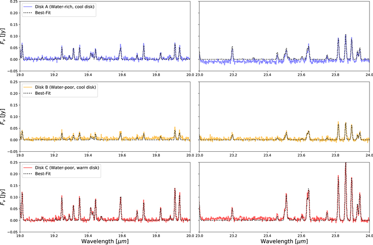
Figure 6. Portion of the best-fit models (black dotted line) superimposed on the continuum-subtracted spectra of the simulated disks (colored line).
Download figure:
Standard image High-resolution image
Figure 7. Continuum-subtracted portion of the Spitzer/IRS spectrum of DK Tau (black) showing the three water bands used in Banzatti et al. (2020) to measure the water-to-organics line ratio. The simulated JWST/MIRI spectra (colored lines, Section 4) highlight that each band includes multiple H2O transitions, a vertical dotted line shows the strongest one for which the flux is reported in the paper.
Download figure:
Standard image High-resolution image5. Summary and Discussion
In this paper, we aimed at testing the scenario put forward in Banzatti et al. (2020) that smaller dust disks have larger H2O/HCN line flux ratios (and larger H2O over accretion luminosity ratios) due to more efficient inward drift of icy pebbles. To this end, we have selected three Taurus disks that have very similar stellar properties but span a factor of 10 in their ALMA-inferred dust disk radii, a factor of 5 in their H2O/HCN line flux ratios, and 1 order of magnitude in their  /Lacc0.6 ratios. According to the models of Kalyaan et al. (2021), these observed ratios translate into a factor of ∼5 difference in the inner water vapor mass of these disks. We have then used CLIcK (Liu et al. 2019) to model the water emission in the Spitzer/IRS medium-resolution (R ∼ 700) spectra of the selected disks and retrieved best-fit values and associated uncertainties for the column density, temperature, and emitting radius of the water vapor emission. In addition, we have simulated JWST/MIRI (R ∼ 3000) disk spectra that differ in their water column density by a factor of 5 and applied to them our retrieval approach. Our main findings can be summarized as follows:
- 1.At the Spitzer resolution, uncertainties on the water column density are too large, up to 0.8 dex for the faintest water spectrum of IQ Tau, that we do not resolve the expected difference in water abundance in the selected Taurus disks. Additionally, the water-emitting radius from the IQ Tau disk, remains unconstrained.
- 2.When we fix the water emitting radius for IQ Tau to 3.0 au, the same as the one inferred for the other two Taurus disks, we find that its water column density is a factor of ∼5 lower than that of the source with the strongest water spectrum, DK Tau. This suggests that reducing uncertainties is critical to test the anticorrelation between H2O/HCN flux ratio and the dust disk ratio.
- 3.At the increased JWST/MIRI resolution and sensitivity, uncertainties in the log of the retrieved water column densities reduce to 0.1–0.2 dex, which is sufficient to discriminate between a factor of 5 difference in the water column density (Table 3).
Among the disks selected for this study, BP Tau will be observed as part of the JWST/MIRI Guaranteed Time Observation program (#1282, PI: Th. Henning) while IQ Tau will be observed in a General Observation program (#1640, PI: A. Banzatti) at high S/N ≥100. DK Tau is not currently scheduled to be observed but, given its rich water spectrum, our estimated uncertainty on the water column density is already relatively low, similar to what JWST can achieve on fainter water spectra (Table 2). Hence, applying our approach to the JWST/MIRI spectra of BP Tau and IQ Tau will enable testing if their different H2O/HCN line flux ratios truly translate into a difference in the water column density ratio.
Along with JWST spectroscopy, deeper/higher-resolution observations with ALMA will be also necessary to test the predictions put forward in Kalyaan et al. (2021). Among our selected disks, only the largest millimeter disk of IQ Tau has a reported gap at ∼40 au while the BP Tau and DK Tau disks appear smooth at the resolution and sensitivity of the Taurus survey by Long et al. (2019). Kalyaan et al. (2021) predict that the most effective gap falls between 7 and 15 au for pebbles between 3 and 10 mm in size and between 30 and 60 au for smaller pebbles. As the ALMA observations from Long et al. (2019) likely probed ∼1 mm-sized grains, the gap in IQ Tau appears to be in perfect agreement with the theoretical predictions. BP Tau and DK Tau might indeed have become smaller dust disks because they lack an efficient pressure bump at large radial distances. Still, BP Tau has a larger dust disk than DK Tau and its inner regions are less water-rich than DK Tau. One possibility is that planetesimal formation outside the snowline was more efficient for BP Tau than DK Tau. Alternatively, the disk of BP Tau might have a closer-in yet-to-be-discovered inner gap that precludes some of the outer icy pebbles to cross the snowline. Future ALMA observations at higher resolution and sensitivity may be able to discover such a close-in gap.
Efficient inward drift of icy pebbles and the release of volatiles at their respective evaporation lines pollutes the disk gas with heavy elements. As recently shown in Scheider & Bitsch (2022) this physical process affects the heavy element content of emerging giant planets. Hence, constraining the efficiency of inward drift is not only relevant to understand what type of planets can form but also what their composition is.
I.P. and M.J. acknowledge support from a Collaborative NSF Astronomy & Astrophysics Research grant (ID: 1715022). Y.L. acknowledges the financial support by the Natural Science Foundation of China (grant No. 11973090). This material is based upon work partly supported by NASA under Agreement No. NNX15AD94G for the program "Earths in Other Solar Systems" and under Agreement No. 80NSSC21K0593 for the program "Alien Earths". The results reported herein benefited from collaborations and/or information exchange within NASA's Nexus for Exoplanet System Science (NExSS) research coordination network sponsored by NASA's Science Mission Directorate.
Facilities: Spitzer (IRS) - , JWST(MIRI). -
Software: astropy (Astropy Collaboration et al. 2013).
Appendix A: The Different Continuum Emission from DK Tau and BP Tau
As discussed in Section 2 DK Tau and BP Tau are located at the same distance and have the same stellar luminosity according to Long et al. (2019). Still, their mid-infrared flux densities are different by a factor of 2 (see also Figure 2), a factor that cannot be explained by the comparatively faint DK Tau B companion. While it is not the goal of this paper to fit the continuum spectral energy distribution (SED) of individual systems, we explore which disk parameters might affect the SED at IR wavelengths.

Figure 8. Baseline SED model (black line) and variations summarized in Table 4. Varying the disk scale height has a large impact on the SED at the wavelengths covered by Spitzer/IRS.
Download figure:
Standard image High-resolution imageWe use the radiative transfer code Hochuck3D (Whitney et al. 2013) to compute a set of SED disk models for a star with stellar mass 0.5 M⊙, temperature 3800 K, and luminosity 0.45 L⊙ located at a distance of 129 pc. These values are chosen because they are representative for DK Tau A and BP Tau, see Table 1. The geometry is that of a flared accretion disk with two dust layers: a surface with small grains ranging in size from 0.01–1 μm and a midplane with grains 0.01–1000 μm. For the dust composition and optical constants we follow DSHARP (Birnstiel et al. 2018). Our fiducial disk model (Model A) has a dust inner radius of 0.1 au, an outer dust radius of 30 au, and disk inclination of 30°, the latter two quantities being in between those of DK Tau A and BP Tau (Table 1). The total dust disk mass is taken to be 8 × 10⁻⁵ M⊙, consistent with the DK Tau A and BP Tau values given the uncertainties in converting millimeter flux densities into dust masses (Pascucci et al. 2016). On top of this fiducial model we apply the following variants: a reduction in accretion luminosity by a factor of 2 (Model B), a factor of 2 smaller dust outer radius (Model C), a factor of 3 lower disk inclination (Model D), an increased scale height (Model E), and a reduced flaring index (Model F), see Table 4 for details. Except for the unknown flaring index and scale height, the other variations are meant to encompass the possible differences in stellar and disk properties between DK Tau A and BP Tau, see the discussion in Section 2. Figure 8 summarizes our results and shows that only a change in the disk scale height and/or flaring index affects the mid-infrared flux density by a factor ≥2. Indeed, as reported in Furlan et al. (2006), BP Tau and DK Tau A have different infrared spectral indices, indicating different amounts of flaring and dust settling. Sargent et al. (2009) also find different proportions of large versus small and amorphous versus crystalline grains when modeling the dust features detected in the low-resolution Spitzer/IRS spectra. In that analysis, DK Tau stands out as one of six disks, among the 65 modeled, with prominent crystalline forsterite features. Finally, it is worth mentioning that the SED of BP Tau, along with selected gas line fluxes, was also modeled as part of the DIANA project (Dionatos et al. 2019; Woitke et al. 2019). This extensive modeling identified the need for a tenuous but vertically extended inner disk out to ∼1.3 au, which casts a shadow on an outer massive disk. Such a tenuous inner disk might explain why the Spitzer spectrum of BP Tau is more similar to that of IQ Tau in spite of IQ Tau being ∼2 times fainter and its disk being closer to edge-on. The detection of a red high-velocity (∼120 km s−1) component in the [O i] 6300 Å line profile of BP Tau (Banzatti et al. 2019; Simon et al. 2016) lends support to the existence of a tenuous inner disk. Such a component is not detected toward DK Tau A (Banzatti et al. 2019; Simon et al. 2016) suggesting that at least this disk, IQ Tau was not observed, has a full dust inner disk that blocks the view of the jet emission moving away from the observer.
While carrying out the SED models summarized in Table 4, we also compiled the broadband photometry for DK Tau A and BP Tau to carry out an independent assessment of the stellar bolometric luminosity. By-eye fitting of the short-wavelength part of the SED with Kurucz stellar models gives a value for BP Tau of ∼0.6 L⊙, consistent with the stellar+accretion luminosity reported in Table 1 and with the value obtained in the DIANA project (Dionatos et al. 2019). Interestingly, DK Tau A shows strong near-infrared J-band emission, which, if assumed to be solely from the star+accretion and included in the fit, raises the bolometric luminosity to ∼1 L⊙, ∼60% more than that of BP Tau. Determining whether there is a real/significant difference in the bolometric luminosity of DK Tau A and BP Tau requires a broader spectroscopic coverage than that used in Herczeg & Hillenbrand (2014) and to properly take into account the accretion luminosity contribution. If the difference exists, it should be taken into account when investigating the origin from the different amounts of mid-IR continuum emission from the two sources.
Appendix B: Best Fits for the BP Tau and IQ Tau Spitzer/IRS Spectra
Here, we provide the figures showing the best-fit models and parameter uncertainties for the BP Tau (Figure 9) and IQ Tau (Figure 10) Spitzer/IRS spectra. The best-fit model for DK Tau is in the main text. In these figures, the best fit is shown with a black dotted line on top of the continuum-subtracted spectrum (solid colored line). The three rightmost panels in each figure show the Bayesian probability distributions for the water column density ( ), emitting radius (Re
), and temperature (T) with the best-fit value indicated by a blue vertical dashed line. The shaded gray region provides the 68% area used to calculate the 1σ confidence intervals for each input parameter. These best-fit values and 1σ uncertainties are also summarized in Table 4.
), emitting radius (Re
), and temperature (T) with the best-fit value indicated by a blue vertical dashed line. The shaded gray region provides the 68% area used to calculate the 1σ confidence intervals for each input parameter. These best-fit values and 1σ uncertainties are also summarized in Table 4.

Figure 9. Same as Figure 4 but for BP Tau.
Download figure:
Standard image High-resolution imageTable 4. Baseline SED Model (Model A) and Variations
| Model | Lacc | Rout | i | Flaring | H100 |
|---|---|---|---|---|---|
| L⊙ | (au) | (deg) | (au) | ||
| A | 0.15 | 30 | 30 | 1.15 | 10 |
| B | 0.075 | 30 | 30 | 1.15 | 10 |
| C | 0.15 | 15 | 30 | 1.15 | 10 |
| D | 0.15 | 30 | 10 | 1.15 | 10 |
| E | 0.15 | 30 | 30 | 1.15 | 20 |
| F | 0.15 | 30 | 30 | 1.05 | 10 |
Notes. See the text for details on other input parameters. H100 is the disk scale height at 100 au.
Download table as: ASCIITypeset image
Appendix C: Sample of Water Line Blends
In Table 5 we provide a breakdown of the blends of selected water lines observed at the Spitzer resolution and within the wavelength range covered by JWST/MIRI. Several of these blends will be resolved at the MIRI MRS resolution.
Figure 10. Same as Figure 4 but for IQ Tau. Note how the emitting radius (Re ) is unconstrained for this source.
Download figure:
Standard image High-resolution image
Table 5. Sample of Water Line Blends
| Spitzer λ | λ | Transition | Aul | Eup |
|---|---|---|---|---|
| (μm) | (μm) | (s−1) | (K) | |
| 17.10 | 17.103 | 125 8 → 112 9 | 3.78 | 3283.8 |
| 17.117 | 1313 0 → 1212 1 | 110.0 | 3259.5 | |
| 17.141 | 168 8 → 157 9 | 42.5 | 6053.7 | |
| 17.22 | 17.209 | 96 4 → 83 5 | 0.339 | 2347.0 |
| 17.219 | 123 9 → 112 10 | 2.61 | 3029.9 | |
| 17.235 | 159 7 → 148 6 | 54.4 | 5820.3 | |
| 17.36 | 17.323 | 168 9 → 157 8 | 41.6 | 6052.0 |
| 17.358 | 112 9 → 101 10 | 0.962 | 2432.5 | |
| 17.374 | 1312 2 → 1211 1 | 93.2 | 5881.7 | |
| 17.405 | 1410 5 → 139 4 | 66.0 | 5643.4 | |
| 23.90 | 23.816 | 83 6 → 70 7 | 0.609 | 1447.6 |
| 23.860 | 98 1 → 87 2 | 31.6 | 2891.7 | |
| 23.895 | 84 5 → 71 6 | 1.04 | 1615.3 | |
| 23.930 | 116 6 → 105 5 | 16.5 | 3082.7 | |
| 23.943 | 115 6 → 104 7 | 9.99 | 2876.1 | |
| 28.40 | 28.409 | 86 2 → 75 3 | 14.5 | 2031.0 |
| 28.427 | 86 3 → 75 2 | 14.5 | 2031.0 | |
Download table as: ASCIITypeset image
Footnotes
- 8
The companion could be on a lower eccentricity orbit to truncate the more extended gaseous disk (e ∼ 0.3, Rota et al. 2022).
- 9
As mentioned at the beginning of this section DK Tau B contributes less than 10% to the broadband mid-infrared flux and therefore cannot explain alone the factor of 2 difference in the Spitzer spectra.
- 10
- 11
As in previous modeling, this is a constant number density within the emitting radius.