


Abstract
A major unresolved issue in solar physics is the nature of the reconnection events that may give rise to the extreme temperatures measured in the solar corona. In the nanoflare heating paradigm of coronal heating, localized reconnection converts magnetic energy into thermal energy, producing multithermal plasma in the corona. The properties of the corona produced by magnetic reconnection, however, depend on the details of the reconnection process. A significant challenge in understanding the details of reconnection in magnetohydrodynamic (MHD) models is that these models are frequently only able to tell us that reconnection has occurred, but there is significant difficulty in identifying precisely where and when it occurred. In order to properly understand the consequences of reconnection in MHD models, it is crucial to identify reconnecting field lines and where along the field lines reconnection occurs. In this work, we analyze a fully 3D MHD simulation of a realistic sunspot topology, driven by photospheric motions, and we present a model for identifying reconnecting field lines. We also present a proof-of-concept model for identifying the location of reconnection along the reconnecting field lines, and use that to measure the angle at which reconnection occurs in the simulation. We find evidence that magnetic reconnection occurs preferentially near field line footpoints, and discuss the implications of this for coronal heating models.
Export citation and abstract BibTeX RIS

Original content from this work may be used under the terms of the Creative Commons Attribution 4.0 licence. Any further distribution of this work must maintain attribution to the author(s) and the title of the work, journal citation and DOI.
1. Introduction
Magnetic reconnection is a ubiquitous process in the solar corona, and is ultimately responsible for nearly all of the important dynamical processes in the solar atmosphere. During reconnection, magnetic field lines exchange their connectivity, and convert magnetic energy into thermal and/or kinetic energy. Small-scale reconnection is thought to be responsible for phenomena such as the heating of the solar corona to its multimillion degree temperatures (Parker 1972; Klimchuk 2006, 2015), the formation of prominences via thermal nonequilibrium (Antiochos & Klimchuk 1991; Antiochos et al. 1999, 2000), and the acceleration of charged particles during solar flares (Knizhnik et al. 2011; Dahlin et al. 2017). On a large scale, reconnection is thought to result in explosive solar phenomena, such as coronal mass ejections (CMEs; Sturrock 1989; Titov et al. 2008; Karpen et al. 2012). The challenge in understanding the role of magnetic reconnection is the incredible scale separation between the kinetic scale, where diffusion enables the breaking of the frozen-in condition, to the global scale, where the consequences of the reconnection are manifest. The diffusion region can have scales likely of the order of centimeters in the corona, while erupting prominences can have lengths of order 1010 cm. While particle-in-cell simulations can resolve the former scales, they are unable to model entire active regions, to study the consequences of reconnection. In contrast, magnetohydrodynamic (MHD) models can be used to model the entire Sun and/or heliosphere, but are computationally unable to resolve the kinetic scales. This lack of a global model that can study both cause and effect makes understanding the properties of magnetic reconnection very challenging.
Nevertheless, progress has been made on MHD models in terms of understanding the behavior of magnetic reconnection on small scales. In particular, numerous studies have indicated the importance of the shear angle at which reconnection occurs, which is sometimes referred to as the onset condition (Leake et al. 2020). This angle can be directly related to the efficiency and amount of energy released by the reconnection process, having consequences for nanoflares (Parker 1972; Klimchuk 2006, 2015; Leake et al. 2020), flux tube merging interactions and instabilities (Dahlburg et al. 1992; Linton et al. 2001), and CMEs (Leake et al. 2022).
In addition, models of prominence formation have indicated that the location of the reconnection along loops can have important consequences for the presence—or lack thereof—of cool material in the corona. These models argue that if the heating due to, say, a reconnection event is sufficiently localized near the chromosphere, the evaporation of the chromospheric plasma toward the top of the loop will result in increased radiative cooling at the apex, since radiative cooling is proportional to density squared. Since the heating at the top of the loop is constant, by assumption, the energy balance may be disrupted, resulting in the now high-density plasma at the loop apex undergoing catastrophic cooling (Antiochos & Klimchuk 1991; Antiochos et al. 1999, 2000; Klimchuk et al. 2010). In the presence of a dip in the magnetic field, cool plasma can be sustained against gravity by the magnetic tension force, directed opposite gravity. This cool plasma is often called a prominence. In magnetic field structures lacking a dip, 3 the heavy, cool plasma would fall down along the loop, being observed as coronal rain (e.g., Mason et al. 2019).
The challenge in studying the onset angle or height of magnetic reconnection is that MHD models of active regions are typically only easily able to identify the global consequences of reconnection, or to state whether or not reconnection has occurred. They are not easily able to identify the location of reconnection, unless the topology contains special regions, such as null points or separatrix and quasi-separatrix layers (Aulanier et al. 2006; Démoulin 2006; Baker et al. 2009; Baumann & Galsgaard 2013; Wyper & Pontin 2014; Boozer 2019; Pontin & Priest 2022), where strong current sheets develop following even minimal stressing. In models with simpler topologies, identifying magnetic field lines that reconnect is very difficult because (1) once reconnected, the identity of the field line is altered, and (2) field lines move in response to applied forces, so even in the absence of reconnection, uniquely identifying a given field line requires advecting the seed point of the field line–tracing algorithm with the velocity flow. Thus, tracing a field line from a seed point that is fixed in time will, in general, produce different field lines at each time step, if there is a nonzero velocity at that point. This makes it difficult to identify whether field lines traced from a given point change their shape due to local forces or reconnection, or whether they were already fundamentally different due to processes occurring earlier and elsewhere.
To address this problem, Knizhnik & Reep (2020) devised a simulation in a Parker (1972) uniform field configuration and applied driving motions at only one boundary, keeping the other boundary line tied and fixed with zero velocity. By tracing magnetic field lines from fixed positions on the fixed boundary, and comparing the expected displacement of the driven ends of the field lines to their actual displacement, they were able to identify reconnecting field lines and quantify the frequency of their reconnection. Building on this model, Knizhnik et al. (2020) were able to use repeated reconnection events on specific field lines and in clusters of field lines to model the plasma response to these heating events using 0D hydrodynamic modeling. Nevertheless, a key factor in realistic models of the corona is the expansion and curvature of the magnetic field in the corona, which was missing in the Parker (1972) models. In this paper, we use a realistic magnetic topology in an MHD simulation of a coronal magnetic field driven by photospheric motions to identify reconnecting magnetic field lines. We determine where along the field lines magnetic reconnection occurs and whether there is a critical angle at which reconnection sets in.
This paper is organized as follows. Section 2 describes the MHD simulation, including the initial and boundary conditions. Section 3 describes the procedure for identifying the reconnecting field lines in the simulation, and the techniques used to identify where the reconnection occurs and what the angle of reconnection is. Section 4 describes the distribution of the angles and locations determined from all of the reconnecting field lines, and Section 5 explores the assumptions inherent in the techniques used and discusses the consequences of our results.
2. Numerical Model
For this work, we analyze two snapshots from the simulation presented in Knizhnik et al. (2017b) and Schuck et al. (2022). For completeness, we include here a general description of the simulation setup.
2.1. The ARMS Code
Our simulation solves the equations of ideal MHD using the Adaptively Refined Magnetohydrodynamics Solver (ARMS; DeVore & Antiochos 2008) in three Cartesian dimensions. The equations have the forms:


In these equations, ρ is mass density, T is temperature, P is thermal pressure, γ is the ratio of specific heats, v is velocity, B is the magnetic field, and t is time. We close the equations via the ideal gas equation,

where R is the gas constant. Our simulation has no explicit resistivity, but the minimal, though finite, numerical dissipation of ARMS allows reconnection to occur at electric current sheets associated with discontinuities in the direction of the magnetic field.
2.1.1. Initial and Boundary Conditions
Our simulation domain has the size Lx = Ly = 7.0, Lz = 2.0, resolved with 384 cells in each of the horizontal directions and 128 cells in the vertical direction. The magnetic field at the photospheric boundary of our simulation is given by
where r2 = y2 + z2 is the cylindrical radial coordinate on the photospheric surface, B0 = −4, B+ = 60, B− = 15, r+ = 2, r− = 4, λ+ = 0.5, and λ− = 1. A line plot and 2D map of Bph(r) is shown in Figure 1. The polarity inversion line (PIL) is situated at r = 2, and the initial coronal magnetic field is calculated by numerically solving

subject to the boundary condition Equation (2.6).

Figure 1. Top: Bph(r) given by Equation (2.6). Bottom: contour plot of Bph(r) at the photosphere of the simulation.
Download figure:
Standard image High-resolution imageWe drive the magnetic field in our MHD simulation with a photospheric velocity profile that contains 199 vortical cells on the bottom plate, as shown in Figure 1 of Knizhnik et al. (2017b; and depicted for one of the snapshots analyzed in this study in Figure 2). Each twist cycle for each cell consists of a slow ramp-up phase, followed by a slow decline phase (Knizhnik et al. 2015, 2017a, 2017b, 2018, 2019; Knizhnik & Reep 2020; Knizhnik et al. 2020). These velocities are loosely meant to mimic supergranular driving. Analytically, the horizontal velocity of each cell is given by

with  being the vertical direction (with x and y in the photospheric plane) and r the radial coordinate centered on each cell. Here,

is the temporal profile of each cell having the period τ = 0.572 tA , with tA = 1 being the dimensionless Alfvén crossing time and
with κ specifying the sense of rotation of each cell based on the value of a random number p ∈ [0, 1], such that
Each photospheric cell having the radius a0 = 0.125 is resolved with 14 numerical grid points across its diameter. In this way, the photospheric motions inject energy into the coronal magnetic field and drive copious magnetic reconnection in the corona. Crucially, all of the driving is contained within the PIL, and all components of the photospheric velocity are set to 0 outside the PIL. The magnetic field at the bottom boundary is line-tied, moving only in response to the imposed flows. The consequences of this will be discussed in Section 3. At the top boundary, the magnetic field is allowed to move freely.

Figure 2. Sample magnetic field lines (green) traced from the photospheric boundary at t = t1. The contour shading (red/blue) shows the horizontal driving velocity on the photosphere. The black circle is the PIL.
Download figure:
Standard image High-resolution image3. Methodology
For this study, we analyze two snapshots from this simulation, taken well into the evolution of the model, at times t1 = 25.7800 tA and t2 = 25.7807 tA . This is about 30 rotation cycles into the driving phase of the simulation. These two times are separated by 14 simulation time steps, each of which are calculated to satisfy the Courant–Friedrichs–Lewy (CFL; Courant et al. 1928) condition, with a CFL number of 0.4. At both of these time steps, a grid of 401 × 401 field lines is traced on the bottom surface using the field line–tracing suite that is built into ARMS (Wyper & DeVore 2016). A subset of these field lines is shown in Figure 2. The field lines traced from near the center and the edges of the photospheric boundary go up and leave through the top of the simulation domain. These field lines correspond to open field regions, as discussed in Knizhnik et al. (2017b). The rest of the field lines correspond to the magnetically closed corona. The structure in these field lines is produced by driving-induced reconnection (see L. K. S. Daldorff et al., 2022, in preparation). For the case where all of the photospheric vortices rotate in the same sense (κ = 1; Knizhnik et al. 2017b), long, sheared filament channels are produced above the photospheric PIL.
Although the seed locations of the 401 × 401 field lines are the same at the two time steps t1 and t2, the field lines traced from these points are not, in general, the same field lines. Field lines starting at an arbitrary point
r
(t = t1) are advected to a different point  by the horizontal velocity given by Equation (2.8). Thus, the same seed point
r
at the time steps t1 and t2 will not, in general, seed the same field line, unless the velocity at
r
is identically 0 in the entire interval [t1, t2]. This is the case for all of the field lines traced from outside the PIL, where all components of the velocity are 0. Therefore, for the two snapshots taken at t1 and t2, we initially consider only the seed points that are outside the PIL, as these correspond to the same field line at both time steps (in the absence of magnetic reconnection). For simplicity, we also only consider field lines that are closed at both ends at both time steps.
by the horizontal velocity given by Equation (2.8). Thus, the same seed point
r
at the time steps t1 and t2 will not, in general, seed the same field line, unless the velocity at
r
is identically 0 in the entire interval [t1, t2]. This is the case for all of the field lines traced from outside the PIL, where all components of the velocity are 0. Therefore, for the two snapshots taken at t1 and t2, we initially consider only the seed points that are outside the PIL, as these correspond to the same field line at both time steps (in the absence of magnetic reconnection). For simplicity, we also only consider field lines that are closed at both ends at both time steps.
3.1. Identifying Reconnecting Field Lines
To determine whether the field line starting at the seed point r o (which is outside the PIL) has reconnected, we compare the expected displacement of the other driven footpoint r i with its actual displacement. Over the interval dt = t2 − t1, the expected displacement of the footpoint is given by

whereas the actual displacement is given by

Since the field lines at the photosphere are line-tied in our model (Knizhnik et al. 2015, 2017a, 2017b, 2018, 2019), and move only in response to the imposed flows, the only way for Dactual not to equal Dexpected is if a field line has reconnected. In this case, the displacement is due to a change in the connectivity of the field line, not to ideal motions. From these arguments, a field line originating from a seed point r o is considered to have reconnected if

To account for potential numerical errors in the field line tracing causing apparent reconnections, we modify the condition in Equation (3.3) to be

Testing has shown that the results are not quantitatively different for different values of α, but the largest reconnection events are likely to be the most energetically interesting, so we take α = 3 for the rest of this study. Using a Parker (1972) topology, Knizhnik & Reep (2020) and Knizhnik et al. (2020) employed this technique to analyze the frequency of magnetic reconnection and the plasma response to the reconnection.
Figure 3 shows plots of the expected and actual field line displacement of the inner footpoint r i from Equation (3.1) for each closed field line outside the PIL. The displacement is mapped onto the location of the seed point r o outside the PIL. To obtain the seed points of the field lines that have reconnected, we plot in Figure 4 the displacement of only the driven footpoints r i that satisfy the condition of Equation (3.4). There are approximately 15,000 such reconnecting field lines. Crucially, at least part of the field line originating at r o is actually the same field line at both times t1 and t2, because the location of r o is outside the PIL and therefore does not move between the two time steps. Therefore, a field line originating from r o and extending up until the point of reconnection x rx is the same at the two time steps.

Figure 3. Expected (top) and actual (bottom) displacements of the driven ends r i of the field lines, starting at seed points r o mapped to the locations of r o .
Download figure:
Standard image High-resolution image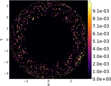
Figure 4. Actual displacements of the driven ends r i of only the reconnecting field lines, starting at seed points r o mapped onto r o . The reconnecting field lines satisfy the condition of Equation (3.4).
Download figure:
Standard image High-resolution imageHaving identified the seed points generating field lines that reconnect between t = t1 and t = t2, we obtain the location of the reconnection event x rx using two different techniques.
3.2. Reconnection at the Location of Bifurcation
One simple way of identifying the location of reconnection is to assume that the time interval dt is so short that the field lines have not had time to undergo other reconnection events, and that the new segment of the field line produced after reconnection is a good representation of the companion preexisting field line prior to the reconnection event. This assumption is reasonable for extremely short time intervals, and will become increasingly less justified as the time interval increases. In our simulation, dt is only 0.1% of the rotation period, meaning that the driving has not had much time to generate additional reconnection events. For a typical supergranular lifetime of about 24 hr (Rieutord & Rincon 2010), the average delay between reconnection events of about 100 s (Klimchuk 2015; Knizhnik & Reep 2020) is about 0.1% of the lifetime of the driver. We therefore expect that, on average, only a single reconnection event will occur for the field lines between our two time steps. Rigorously testing this assumption is outside the scope of this paper, since the technique is primarily a proof of concept here.
Consider a field line that reconnects somewhere along its length with another field line and changes its connectivity, as shown in the left panel of Figure 5. In the absence of any imposed velocity at the footpoint, below the reconnection point the field line segment will be the same before and after the reconnection. Immediately after the reconnection, the segment above the reconnection point will go off in a different direction from the original field line, and one can define a distance ds(n) between the two segments at the two different times. Here, n is the step number along the field lines (which are traced with the same step size), so that ds(n) is the distance between the two segments at step n. The key to this method is that the gradient of ds(n) will be maximized at the location of the reconnection event. While the separation is zero throughout the segment below the reconnection location, and can be quite large far above the reconnection location, its rate of change along the curve will be greatest where the reconnection occurs. This is shown in the right panel, where we plot an approximate shape of the gradient of ds(n) for this cartoon model. The gradient starts at 0 and then increases rapidly at the reconnection location, before decreasing and plateauing at some small value. We can write the step number along the field line where the reconnection is assumed to have occurred as

where n is the step number and sk (n; ti ) is the position s along the reconnecting field line, starting from the fixed seed point k at the time step ti . The seed point k and the step number nrx therefore uniquely identify the three spatial coordinates at which reconnection occurs.
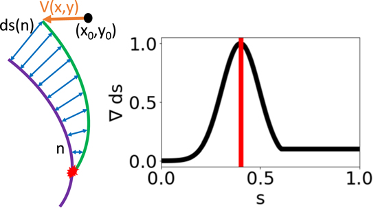
Figure 5. Left: cartoon showing a field line before (purple) and after (green) reconnection. The bottom portion of the reconnecting field line is shared during the two time steps, and the spacing between the "before" and "after" field lines is defined as ds(n) along the length of the "before" field line, where n is the step number along the field line (for the same step size along the two field lines). The upper end of the green field line arrives at its location due to some imposed velocity, having at the previous time step been at the location (x0, y0). Right: the gradient of ds(n) will start at 0, where the two field lines share a segment, and then increase rapidly near the reconnection point, where the two field lines diverge the quickest. As the segments of the field lines beyond the reconnection event move farther apart, their separation increases, but, in the absence of additional reconnection events, the gradient of the separation will decrease and plateau at some small value.
Download figure:
Standard image High-resolution imageThe method described above is applied to a reconnecting field line, as shown in Figure 6. Here, the separation distance between the "before" and "after" field lines (red curve) has been smoothed using a seven-point Savitsky–Golay filter, to remove many of the spikes caused by waves and the discrete field line–tracing step size. This is done primarily to avoid artifacts when taking the gradient of the separation. The gradient of the separation distance (blue) has occasional oscillations, but also a clear signature of where the separation distance increases most rapidly. For cases where there is a large negative gradient in the separation distance, this corresponds to the field lines coming closer together, which is not what is expected following a reconnection event. We therefore consider the location of the maximum of the signed gradient of the separation to be the location of the reconnection.

Figure 6. Calculation of the bifurcation method from the field lines plotted in the bottom right panel of Figure 7. The separation between the field line before and after reconnection, ds (red), is plotted along with the gradient of ds (blue). The location of the reconnection is identified at the location of maximum gradient (black line).
Download figure:
Standard image High-resolution image3.3. Reconnection at the Location of Closest Distance
The second method that we use to determine the location of reconnection is to identify the second field line at t = t1 that participated in reconnection. This is done as follows.
Consider again the post-reconnection green field line in Figure 5. Its driven (upper, in the figure) footpoint arrives at its post-reconnection location due to the imposed boundary flow v (x, y) from its previous location at (x0, y0). Therefore, tracing a field line from (x0, y0) at the previous time step would have produced the field line with which the original purple field line reconnected. This would create two known field lines at the same time step that reconnect with each other. It is reasonable to suppose that the reconnection occurs where the two field lines are closest together. In the absence of footpoint driving, the current density would likely be largest at the reconnection location, but the current density signal dominates near the driver, so this would be a biased threshold to use here.
Since the process described in Section 3.1 identifies the post-reconnection field line at t = t2, it remains to advect the driven end of the field line back to the position at t = t1, by using the known velocity field and the time increment. Thus, the coordinates of the second, reconnecting field line at t = t1 are

and

The velocity components are interpolated to the locations (x(t2), y(t2)), as these are, in general, not defined on the original simulation grid. We then use the streamtracer Python package to trace a field line from (x0(t1), y0(t1)) and find the step number nrx along the two field lines, where distance between the two reconnecting field lines at t = t1 is minimized.
3.4. Determination of the Angle and Location of Reconnection
Once the step number along the two field lines where the reconnection is assumed to have occurred has been identified, the location of the reconnection event is straightforwardly obtained from the coordinates of the field lines at nrx. We can then calculate the fractional half-length of the reconnecting field line as
where L/2 is the half-length of the pre-reconnection field line, dl is the length increment for step n, and the subscript i on the fractional half-length denotes the method used: i = 1 for the bifurcation method described in Section 3.2; i = 2 for the minimum distance method described in Section 3.3.
To obtain the reconnection angle, the magnetic field vector components are interpolated to that location on the two field lines and the angle of reconnection is calculated via

Here,  and
and  are the magnetic field vectors at the location of reconnection nrx, and the subscript i on the reconnection angle θ denotes the method used: i = 1 for the bifurcation method described in Section 3.2; i = 2 for the minimum distance method described in Section 3.3. It should be kept in mind that the maximum bifurcation method identifies the reconnection location based on the field lines at two different time steps, while the minimum distance method identifies the reconnection location based on field lines at the same time step.
4. Results
In Figure 7, we plot four examples of using the techniques described in Section 3 to find reconnecting field lines in the simulation and the location of the reconnection, as determined by both the maximum bifurcation and minimum distance methods. The blue field line, plotted at t = t1, was determined to have reconnected based on the criterion in Equation (3.4) and produced the orange field line, plotted at t = t2, which shares a segment with the blue field line. The location of the maximum gradient of the separation between the blue and orange field lines is marked with the black circle. The driven footpoint of the orange field line was then advected back in time from t = t2 to t = t1, based on the imposed flow, and a field line (red) was traced from its location at t = t1 using the streamtracer package. Thus, the red and blue field lines, both traced at t = t1, reconnect with each other to form the orange field line. The likely location of reconnection is the point where the blue and red field lines are closest together, marked with the black star. These reconnection points seem reasonable by eye, and are well representative of the other field line reconnections calculated in our model. In principle, the undriven footpoint of the red field line can be traced at t = t2 to calculate the second new field line produced by the reconnection event. However, given that a grid of fixed field lines has already been used to identify the reconnection, this would be redundant with the field lines already traced from outside the PIL.

Figure 7. Reconnecting field lines shown before and after reconnection. The red and blue field lines reconnect between time steps t = t1 and t = t2 and form the orange field line, which shares a seed point with the blue field line at both time steps. The black dot and star identify the location of the reconnection as determined from the bifurcation and closest-distance approaches, respectively.
Download figure:
Standard image High-resolution imageFor all of the reconnecting field lines in our simulation between time steps t1 and t2, we calculate reconnection angles (Equation (3.9)) and fractional half-lengths (Equation (3.8)) using both methods described above. We show a histogram of the measured angles in Figure 8 and the fractional half-lengths in Figure 9. Both methods find extremely small reconnection angles, with a median angle of about 2° for each. It is, perhaps, unsurprising that the reconnection angle determined by both techniques is approximately the same. Our model does not resolve the kinetic scales needed to treat reconnection accurately, and it does not include adaptive mesh refinement, to enable the reconnecting current sheet to thin down to any realistic aspect ratio. The simulation therefore has no mechanism to suppress reconnection until some critical angle is reached, as would be expected from smaller-scale MHD models that resolve the current sheet in fine detail (Leake et al. 2020). Indeed, numerical diffusion enables reconnection to occur in our model, so the reconnection angle is not expected to play an important role. The location of the reconnection, on the other hand, is likely to be physically meaningful, as determined by our model, even if the exact mechanism and details are not. The location distributions of reconnection events are vastly different as determined by the two methods, though there is a clear preference for events in the bottom 20% of the half-loop. The maximum bifurcation method finds that reconnection occurs throughout the half-loop, with a peak near 0.1, while the minimum distance technique finds that reconnection has a strong preference to occur even closer to the loop footpoints. It is important to note that the normalized scale in this histogram represents the fractional length of only half of the loop, implying that, at least as inferred from these plots, a preference for reconnection near one footpoint or the other cannot be determined. Since the two ends of the loop are asymmetric—one side being driven, while the other is not, and one end being in a region of high magnetic flux and the other not—such a determination would be difficult to connect to more physically realistic scenarios, where the driving and flux distributions are random. In contrast, the location of reconnection along the half-length of the loop in an expanding, realistic magnetic geometry is much more physically meaningful than the same quantity determined for a plane-parallel Parker (1972) magnetic field.

Figure 8. Histograms of the reconnection angles from the bifurcation (top) and minimum separation (bottom) methods. The median reconnection angle is shown with the red vertical line.
Download figure:
Standard image High-resolution image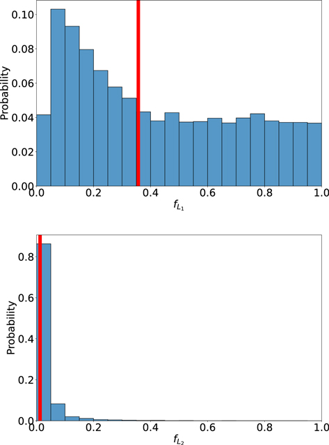
Figure 9. The reconnection locations along the loop from the bifurcation (top) and minimum separation (bottom) methods. The median reconnection location is shown with the red vertical line.
Download figure:
Standard image High-resolution imageGiven this disparity in the locations of reconnection as determined by the two methods, it is worth investigating whether the individual angles and locations found by the two methods are similar. To this end, we show a scatter plot of the angles and locations in Figure 10, along with the Pearson correlation for the two data sets. The angles show a linear trend, but not one that is very statistically significant, indicating that the two methods ultimately find very different values for the angles for each individual reconnection event. The locations determined by the two methods are absolutely not correlated, indicating that the locations of the reconnections found by the two methods are vastly different for each reconnection event.

Figure 10. Scatter plots of the angles θ1 and θ2 (top) and fractional half-lengths  and
and  (bottom), as determined by the maximum bifurcation and minimum separation methods. The red line has a slope of 1 and we quote the Pearson coefficient for the relationship.
Download figure:
Standard image High-resolution imageWe also compared the length distribution of the reconnecting field lines—prior to their reconnection—against the length distribution of all of the closed field lines, as shown in Figure 11. An obvious feature that stands out is the relative dearth of really short field lines reconnecting, relative to their population. This is likely due to the threshold that was set on α in Equation (3.4). In addition, the decrease in reconnecting field lines around a length of 2 relative to their distribution in the entire closed field line set is due to our exclusion of reconnection events that reconnect a closed field line with an open field line. Since our box height is Lz = 2, reconnection events that occur due to field lines that hit the top of the box are not counted in our analysis. With these two caveats, these distributions show that field line reconnections are sampled approximately in proportion, by length, to their prevalence in the simulation domain. In other words, there does not seem to be a preference for long or short field lines to reconnect.

Figure 11. Histograms of the lengths of the reconnecting field lines (top) and all the closed field lines (bottom). The median length is indicated by the red vertical line.
Download figure:
Standard image High-resolution image5. Discussion
In this work, we have presented a new method of using MHD simulations to determine the location and angle of reconnection for magnetic field lines driven at one photospheric footpoint. Our method of driving the field lines only at one end, while keeping them line-tied at the other end, and then tracing field lines from the line-tied end, enables us to uniquely identify at least a segment of the field line that maintains its identity before and after the reconnection event. From the standpoint of energy injection, it is completely equivalent to consider a magnetic field driven at one footpoint with velocity v , or at both footpoints with velocity v /2. Thus, although solar driving is likely to occur at both footpoints of the field line, the energetics of the process, and the location of reconnection, are likely to be insensitive to whether the field is driven at one or both footpoints.
We used two heuristics to identify the location of reconnection, namely (1) the location of maximal bifurcation of the pre- and post-reconnection magnetic field lines, and (2) the location of minimal separation between reconnecting field lines. Both of these heuristics involve several assumptions that may or may not be satisfied. The first requires that the "before" and "after" reconnection time steps are separated by a timescale much smaller than the inverse of the frequency of reconnection. The second adds the additional assumption that the grid size, current density, and width of the associated current sheet play no role in determining whether reconnection occurs, and the only thing that matters is the separation distance. In our model, the largest currents are generated near the drivers, so analyzing the location of reconnection in our model based on the current density is a challenging task. Additional constraints or thresholds for identifying the location of reconnection can be employed in the presence of, for example, explicit localized or anomalous resistivity, preexisting current sheets, or strong twist or shear (Leake et al. 2020). While it is beyond the scope of this paper to test each of these assumptions and scenarios in our simulation, the methods described herein act as a proof of concept for obtaining the properties and statistics of reconnection in line-tied topologies, where one or more of the above-listed assumptions may be valid.
We have used these techniques to determine that there is a strong preference for small-angle reconnection, even smaller than the 10°–30° derived via equating the observed heating to the photospheric Poynting flux (Parker 1983, 1988; Priest et al. 2002; Klimchuk 2006, 2015), and certainly less than the 45° required for the secondary instability of the tearing mode to set in (Dahlburg et al. 1992, 2005, 2006, 2009). Typical estimates of the energy released by reconnection use observed values of the normal magnetic field and flux tube cross section and inferred estimates of the average delay between reconnection events (roughly 100 s; Klimchuk 2015; Knizhnik & Reep 2020). For a reconnection angle of 10°, the canonical energy loss rate of 107 erg cm−2 s−1 can be reproduced (Withbroe & Noyes 1977). Keeping the other observables constant, changing the angle changes the energy per unit area released by reconnection by a factor (Klimchuk 2015)
For θ = 10° and  , this comes out to about five times less energy being released by reconnection than the amount estimated by Withbroe & Noyes (1977) as being necessary to explain the observed losses.
Nevertheless, as argued above, the small reconnection angle measured here is not expected to accurately reflect the real reconnection angle in extremely high resolution MHD simulations. Our model is not designed to support the growth of the long, thin current sheets that are required for reconnection to be suppressed for any amount of time prior to onset (Loureiro et al. 2007; Baalrud et al. 2012; Huang & Bhattacharjee 2013; Pucci & Velli 2014; Del Zanna et al. 2016; Huang et al. 2017; Pucci et al. 2017; Leake et al. 2020). Our model uses numerical resistivity to enable reconnection, and is thus missing the key physics of the process. Klimchuk (2015) argues that the reconnection angle is likely to be similar to the inclination of the field from the vertical at the photosphere. To this end, we plot the inclination angle of the field at the photosphere in Figure 12. A large fraction of the photospheric field is highly inclined from the vertical, far in excess of the 10°–20° required to explain the observed heating. Higher-resolution and smaller-scale MHD simulations are needed to verify the reconnection angle in the presence of fundamental physics, and the techniques presented in this work may prove useful in identifying the location and, therefore, the angle of reconnection in such a regime.

Figure 12. Inclination angle (degrees) of the photospheric magnetic field relative to the vertical. The blue circle is the PIL.
Download figure:
Standard image High-resolution image
The location of reconnection, on the other hand, can be expected to be meaningfully determined by our MHD model. Here, the two techniques somewhat disagreed about the position along the loop at which reconnection occurs, though there is a clear preference for the loop footpoints. While the maximum bifurcation method found reconnection all along the loop, the minimum distance method overwhelmingly localized the reconnection events near the loop footpoints. Our model does, therefore, lend some support to the presence of self-consistent heating that is localized near the loop footpoints. Footpoint heating is commonly thought to be a crucial ingredient for thermal nonequilibrium models of prominence formation (Antiochos & Klimchuk 1991; Dahlburg et al. 1998; Antiochos et al. 1999, 2000; Karpen & Antiochos 2008) and dynamics (Luna et al. 2012), as well as coronal rain (Mok et al. 1990; Froment et al. 2015, 2017; Mason et al. 2019). In the prominence formation paradigm, our model argues that reconnection between closed loops occurs most often near the footpoints, leading to thermal nonequilibrium. Such reconnection could also potentially generate large-amplitude longitudinal filament oscillations (Luna et al. 2014). We also investigated whether there was a correlation between the loop half-length and reconnection location, but were unable to find any meaningful relationship. This fact, combined with the pre-reconnection length distribution of Figure 11, indicates that reconnection is entirely agnostic to loop length. This is likely to be true only down to the current sheet scale, where the aspect ratio of the current sheet is thought to be a critical parameter in reconnection onset (Baty 2017).
It could reasonably be argued that the inability of our model to suppress reconnection preferentially localizes it near the footpoints. Since even small misalignment angles generate a change in connectivity and the driving occurs near the footpoints, Aflvén waves propagating up from the driver will immediately generate sufficient misalignment between adjacent field lines and cause reconnection. This could very well be true, but is likely still representative of the situation in the low corona. The magnetic flux is highest near the bottom of the loop, so regardless of what the reconnection angle is, it is most likely to be achieved there.
One challenge in interpreting the physical implications of our model, given the nondimensional units used for all of the quantities here, is determining what environment or regime our results apply to. In principle, in the absence of gravity, MHD is scale-free, and the choice of any three scales for, e.g., field strength, length, and mass density, constrain the others. This would seem to argue that our results apply completely generally to any boundary-driven system constrained by the choice of three of the fundamental quantities. Nevertheless, the assumptions in our model constrain the results to apply to only closed-field topologies (since open field lines were explicitly ignored). The field line length distribution varies only by a factor of 5–6, making this configuration unlikely to be relevant for something like a helmet streamer loop. We therefore argue that our results apply to a simple low-lying active region, which is perhaps responsible for the chromospheric or transition region "moss" that is thought to overlie these regions (De Pontieu et al. 2009). Our results are certainly not meant to apply to complex magnetic field topologies, such as jets or pseudostreamers.
It is important to acknowledge that the results presented here are not meant to be considered as the final word on the location and angle of reconnection as derived from MHD simulations. In addition to the caveats listed above, the footpoint driving, which is concentrated in the region of highest magnetic flux, may artificially select out locations near the photosphere where the magnetic field has not yet expanded much. Future work will focus on exploring how the simplistic nature of the driving affects these results, and on how the varying field strength along the loops (not seen in the Parker 1972 models) changes the plasma response to reconnection due the changing loop cross section (Reep et al. 2022).
K.J.K. was supported by NASA GSFC's Internal Scientist Funding Model (competitive work package on "Understanding Coronal Heating and the Solar Spectral Irradiance") and by the Office of Naval Research 6.1 Support Program. The research of L.C.C.P. was sponsored by the Office of Naval Research Enterprise Internship Program. The authors would like to thank Jim Klimchuk, the lead of the coronal heating work package team, for helpful discussions, and Lars Daldorff, for the use of his ARMS data-reading code. The authors are also grateful to the anonymous referee, whose comments helped improve the quality and readability of the manuscript.
Software: h5py (Collette 2013) Matplotlib (Hunter 2007), Numpy (Oliphant 2006), Scipy (Virtanen et al. 2020), seaborn (Waskom et al. 2018), streamtracer (https://streamtracer.readthedocs.io/en/stable/).
Footnotes
- 3
See, however, Karpen et al. (2001).