


Abstract
We have obtained constraints on the nanoflare energy distribution and timing for the heating of a coronal bright point. Observations of the bright point were made using the Extreme Ultraviolet Imaging Spectrometer on Hinode in slot mode, which collects a time series of monochromatic images of the region leading to unambiguous temperature diagnostics. The Enthalpy-Based Thermal Evolution of Loops model was used to simulate nanoflare heating of the bright point and generate a time series of synthetic intensities. The nanoflare heating in the model was parameterized in terms of the power-law index α of the nanoflare energy distribution, which is ∝ E−α; average nanoflare frequency f; and the number N of magnetic strands making up the observed loop. By comparing the synthetic and observed light curves, we inferred the region of the model parameter space (α, f, N) that was consistent with the observations. Broadly, we found that N and f are inversely correlated with one another, while α is directly correlated with either N or f. These correlations are likely a consequence of the region requiring a certain fixed energy input, which can be achieved in various ways by trading off among the different parameters. We also find that a value of α > 2 generally gives the best match between the model and observations, which indicates that the heating is dominated by low-energy events. Our method of using monochromatic images, focusing on a relatively simple structure, and constraining nanoflare parameters on the basis of statistical properties of the intensity provides a versatile approach to better understand the nature of nanoflares and coronal heating.
Export citation and abstract BibTeX RIS

Original content from this work may be used under the terms of the Creative Commons Attribution 4.0 licence. Any further distribution of this work must maintain attribution to the author(s) and the title of the work, journal citation and DOI.
1. Introduction
Nanoflare theories of coronal heating posit that the corona is heated through a large number of discrete, relatively low-energy release events, known as nanoflares. It is usually thought that these nanoflares are due to the energy released from reconnection (Parker 1983). However, many possible coronal heating mechanisms are impulsive in nature, and nanoflare models are now often considered to be a phenomenological description for any form of impulsive heating (Klimchuk 2015). Observations that measure the properties of nanoflares, such as their energies and frequencies, can be compared with heating models in order to constrain the underlying physical heating process. A challenge for inferring nanoflare properties is that nanoflares are small by definition, and so individual heating events are not resolved.
In active regions, a number of studies have characterized heating in terms of nanoflare parameters relevant to a Parker-type model of nanoflares (e.g., Warren et al. 2002; Schmelz et al. 2010; Mulu-Moore et al. 2011; Viall & Klimchuk 2011; Reep et al. 2013; Barnes et al. 2016). Such studies conceptualize coronal loops as composed of a large number of unresolved magnetic strands. As these strands are twisted and braided around one another by convective motions and turbulence, the strands reconnect and produce nanoflares.
There is some debate as to whether such strands actually exist. Some researchers argue that high-resolution observations should resolve strands, yet they are not observed (Brooks et al. 2012, 2013; Aschwanden & Peter 2017). Proponents of the strand paradigm dispute these conclusions (e.g., Cirtain et al. 2013; Pontin et al. 2017; Klimchuk & DeForest 2020). For example, Cirtain et al. (2013) found direct evidence for braided field lines in high spatial resolution observations, and Pontin et al. (2017) have argued that the presence of braided field lines does not necessarily lead to a braided appearance in observed intensities. However, the strand model, picturing coronal loops as analogous to the strands of string that make up a rope, makes idealizations that may not be physical. For example, strand-like structures do not need to be stable flux tubes. Instead, they could arise due to plasma instabilities, such as the Kelvin–Helmholtz instability (Antolin et al. 2014). Any filamentary density structures that form are also expected to be mixed by Alfvén waves propagating along loops, leading to a complex density structure (Magyar & Van Doorsselaere 2016).
Despite these complications, as a phenomenological model the strand concept has the practical advantage of specifying the parameters that observations must measure to specify the energy distribution of the nanoflares and their timing. Here, we adopt this traditional view of nanoflare heating and apply it to an observation of a coronal bright point.
Bright points offer several advantages over active regions for understanding coronal heating theories. Bright points are small structures, typically ∼10 Mm in size, and are usually a loop formed over a magnetic bipole (Alexander et al. 2011). This may be compared to active regions, which are ∼100 Mm in size and have very complex magnetic fields. Observational studies have shown that, like active regions, bright points are impulsively heated (Brosius et al. 2008; Schmelz et al. 2013; Raouafi & Stenborg 2014). Although beyond the scope of this paper, the simple geometry of bright points should enable a more direct comparison between heating events and the evolution of the magnetic field than for the complex active regions. For example, bright point heating appears to be driven by canceling magnetic flux or flux emergence (Webb et al. 1993; Schmelz et al. 2013).
The basic outline of our approach is as follows: We use the slot mode of the Extreme Ultraviolet Imaging Spectrometer (EIS; Culhane et al. 2007) on Hinode to measure the observed intensity of spectral lines as a function of time, Iobs(t), for a bright point. The heating of the bright point is modeled using the Enthalpy-Based Thermal Evolution of Loops model (EBTEL; Klimchuk et al. 2008; Cargill et al. 2012a, 2012b). We provide the model with a hypothetical heating function H(t) that represents a time series of nanoflare energy pulses. These nanoflares follow a power-law energy distribution ∝ E−α
characterized by the power-law index α. They occur on each strand with an average frequency f and there are N strands. EBTEL then uses H(t) to compute the time-varying differential emission measure (DEM) expected from the bright point. This DEM describes the temperature distribution of the material along the line of sight. Using the CHIANTI atomic database (Dere et al. 1997, 2019), we convert the theoretical DEM to a model intensity  . Finally, we compared the synthetic and observed intensities to determine the set of parameters α, f, and N that best fit the observations and thereby characterize the nanoflares.
The rest of this paper is organized as follows: Section 2 describes the observations and some instrumental issues related to the EIS slot mode. In Section 3 we discuss the construction of the theoretical heating function, the application of the EBTEL model, and the metrics by which we compare the observed and synthetic intensities. Section 4 considers some of the implications of this work and future directions. The principal results are summarized in Section 5.
2. Instrument and Observations
The main data set for our analysis was obtained using the 40'' slot of EIS on 2008 December 9 starting at 14:50 UT. For this observation the 40'' slot was rastered across three slightly overlapping positions leading to a field of view that is 96'' in the horizontal direction and the full length of the slot, 512'', in the vertical direction. The pointing was centered at solar coordinates (72 8, 5670) relative to the center of the solar disk. Each exposure was about 28 s, and the total cadence to cover the field of view was about ≈90 s. The data set includes 100 exposures and the region was observed for a duration of ≈230 minutes. Of these, two exposures were rejected as the data were of poor quality, and we analyzed the remaining 98 frames. The observed region is near the boundary between the quiet Sun and a coronal hole, and there is a prominent bright point near the center of the frame (Figure 1). This bright point is the focus of our analysis. EIS also observed the same region using the 2'' slit on 2008 December 9 at 11:00 UT. We use the slit data for the density analysis described below.
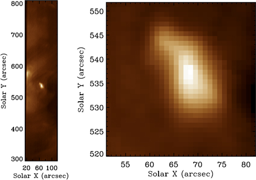
Figure 1. The field of view for the EIS observation in Fe xii 195.12 Å. On the left is the full field of view and on the right is the region focusing on the bright point.
Download figure:
Standard image High-resolution imageEIS slot data are unambiguously related to particular spectral lines, but the spatial and spectral dimensions share the same axis. As a result, the intensity of light that should appear at a given spatial pixel is partially spread out to neighboring spatial pixels. The point-spread function (PSF) that describes this spreading is dominated by the shape of the spectral line. We performed a deconvolution to correct for this smearing out of the intensity.
To perform the deconvolution, we assume that the spectral lines are Gaussian. This is consistent with the high spectral resolution data from the 2'' slit. This is typical for EIS data as the EIS line widths are dominated by the instrumental width. In the EIS slit spectra, the EIS instrumental line width in velocity units is about 40 km s−1 (Hara et al. 2011; Young 2011). In comparison, the thermal line width for iron lines at 1 MK is about 17 km s−1 and there is often a nonthermal broadening of ∼20 km s−1 s−1 (e.g., Chae et al. 1998). This nonthermal broadening is due to waves, turbulence, or other flows along the line of sight. These various contributions to the total line width add in quadrature, so the instrumental width forms the dominant contribution. To better quantify the appropriate line width for the slot, we measured the Fe xii 195.12 Å line intensity and measured the line shape around several small bright features and the fall-off in intensity at the edge of the field of view. This analysis showed that the EIS 40'' slot line width is broader than for the slit, which is consistent with its lower expected spectral resolution, and the slot has a typical line width of 0.038 Å, which is ≈58 km s−1 in velocity units or about 1.7 pixels. Finally, we assume the lines have the same centroid throughout the field of view. This approximation is expected to be reasonable as the Doppler shifts in bright points are typically less than 10 km s−1 or 0.3 spectral pixels, thus remaining well within the peak of the broad Gaussian line shape (Pérez-Suárez et al. 2008).
The observed signal si at pixel i is the sum of the wavelength-integrated intensities I at the 2K positions along the same row of the image weighted by their contribution to the pixel i:

The weights, wi , sum to one.
For our analysis we studied two strong lines that are well separated from other significant spectral lines. These are the Fe xii line at 195.12 Å and the Fe xv line at 284.16 Å. These lines have peak formation temperatures of 1.6 and 2.2 × 10⁶ K, respectively. Limiting our analysis to isolated lines allows us to make the assumption that the signal is due to a single Gaussian. Then, we can derive the weights by integrating the Gaussian line shape over each bin. In practice, using K = 3 pixels on either side of the ith pixel accounts for 97% of the observed intensity, which greatly reduces the number of terms needed, while introducing negligible errors. One can consider Equation (1) as a matrix equation s = W I . In principle, the deconvolution could be accomplished using I = W −1 s . However, small errors are magnified by the inversion and there is no guarantee that the results will lead to positive intensities. Instead, we have used the iterative method of Richardson (1972) and Lucy (1974), which is stable and ensures positive intensities.
3. Analysis
For our analysis we first characterized statistics of the observed bright point intensity. Next we generated synthetic intensities corresponding to an assumed heating function and compared these to the observed intensities. Finally, we adjusted the parameters used to generate the heating function to determine what was required in order to produce model intensities that best resemble what was observed.
We selected bright point pixels in the observation by imposing a threshold, requiring that the median intensity of the pixel be greater than 700 erg cm−2 s−1 sr−1 for Fe xii 195.12 Å, and 400 erg cm−2 s−1 sr−1 for Fe xv 284.16 Å. This threshold identifies 195 pixels as being part of the bright point for Fe xii and 130 pixels for Fe xv. Figure 2 illustrates the selected points for Fe xii.

Figure 2. One frame of the time series of EIS slot images in Fe xii cropped to show the pixels considered as belonging to the bright point.
Download figure:
Standard image High-resolution imageAs we will compare these intensities to a zero-dimensional model, we neglect the spatial distribution of the bright point emission in our analysis and consider instead the statistical properties of the observed intensities. We also neglect the time dependence of the emission in our analysis. That is, from each bright point pixel, we collect a time series of intensity data, but for the analysis we consider only the statistical properties of these data. Some previous studies in active regions have attempted to model the intensity time series using a nanoflare heating function (e.g., Tajfirouze et al. 2016). To match the time dependence requires producing a heating function that not only describes the correct distribution and frequency of nanoflares, but also place them in the same sequential order as observed. Doing so is computationally expensive. Here, we instead analyzed all relevant ∼ 104 bright point intensity measurements as a set independent of location and time. From the observed data, we produced a histogram of the intensity. We then generated synthetic intensities representing a hypothetical heating function and attempted to produce histograms of the synthetic data that matched that of the observed data.
The bright point heating was modeled using the EBTEL hydrodynamic model to simulate nanoflares. EBTEL is a zero-dimensional model that solves the hydrodynamic equations for averaged quantities along a coronal loop (Klimchuk et al. 2008; Cargill et al. 2012a, 2012b). It does this, by solving separate energy equations for the corona and transition region and accounting for the transfer of mass and energy between these regions. Comparisons with one-dimensional loop models have shown good agreement. The accuracy and efficiency of the model make it well suited to comparing various nanoflare heating functions with observations. EBTEL has become a standard tool for simulating nanoflares for comparison with active region observations (e.g., Qiu et al. 2013; Kobelski et al. 2014; Ugarte-Urra & Warren 2014; Tajfirouze et al. 2016).
EBTEL takes as input the loop length and a time-dependent heating function. From images of the bright point and assuming a semicircular loop, we estimated the loop length to be ≈1.1 × 109 cm. The properties of the heating function will be described shortly. From these inputs, EBTEL calculates the coronal and transition region DEMs, as well as related quantities such as the average loop temperature and loop-top temperature. Our analysis uses the DEM outputs from EBTEL, which implicitly contain all of the temperature information. We do not use the average or loop-top temperature outputs. From the total output DEM, we generated synthetic intensities for comparison to the observed intensities. The model intensity for each line was computed by multiplying the DEM by the contribution function G(T) using the data from the CHIANTI atomic database (Dere et al. 1997, 2019) and then integrating over temperature. In order to treat the EBTEL results on the same basis as the EIS observation, we averaged the model intensity time series over 28 s bins to mimic the averaging that occurs in the EIS data due to the exposure time.
In order to determine the nanoflare parameters that best reproduced the observed intensities, we compared the statistical properties of the observed and model intensities. Specifically, we constructed a histogram of the set of the observed intensities from every exposure and every pixel identified as being part of the bright point. The bin size for the intensity histogram was 100 erg cm−2 s−1 sr−1. We then constructed a similar histogram of the model intensities using the same binning. Figures 3 and 4 show examples corresponding to the best fits to the Fe xii and Fe xv data, respectively. To facilitate the comparison, the model and observed histograms were normalized by the total number of data points in their respective data sets. That is, the sum over all the histogram bins is one for each histogram. The match between the observation and theory was quantified using the summed squared differences between the histograms,

where yobs,i
and  are the normalized counts for the observed and model histograms, respectively, in the ith intensity bin, and the sum is over the full intensity range of the histogram.
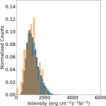
Figure 3. The observed and model intensities were compared statistically on the basis of their histograms. In this example from the Fe xii analysis, the blue and orange histograms show the statistical distributions of the observed and theoretical intensities, respectively. In both cases, the histograms have been normalized by the total number of data points making up the distribution. These results compare to a good fit for the model with α = 2.5, f = 3 × 10⁻⁴ s−1, and N = 330.
Download figure:
Standard image High-resolution image
Figure 4. Same as for Figure 3, but for Fe xv corresponding to the model with α = 2.4, f = 3 × 10⁻⁴ s−1, and N = 220.
Download figure:
Standard image High-resolution imageThis metric was chosen because it is expected to represent how well the statistical properties of the nanoflares match those observed, but without requiring that those nanoflares occur in the same specific sequential order as in reality. A similar approach was used by Pauluhn & Solanki (2007). As mentioned earlier, Tajfirouze et al. (2016) performed an analysis similar to ours for an active region, but they required that the model time series itself match the observed light curve. This led to a resemblance between the observed and synthetic light curves, but required the generation of many more synthetic light curves than our approach and the use of probabilistic neural networks to sift through the data. Although our approach based on statistics will not match the observed light curve, it does capture the essential physics.
A possible modification to our method is to consider metrics other than D for comparing the observed and model intensities. One issue is that D applies an equal weighting to each bin, which tends to underemphasize the comparison in the high-intensity tail of the distribution, where the number of counts is always small. Physically, the tail corresponds to higher energy events and so could lead to a systematic error in α. A variable weighting, or equivalently a varying histogram binning, could be used to increase the importance of the tails. Doing so would increase the computation required by the model, as the model must run for sufficient time to ensure that the tail of the model intensity distribution is statistically populated. We will explore possible computationally tractable alternate metrics in a future work.
The free parameters for the nanoflare heating function were the power-law index of the nanoflare energy distribution α, the number of elemental strands along the line of sight N, and the average nanoflare frequency per strand f. The nanoflare energies were distributed using a power-law distribution p(E) ∝ E−α . The energy range for the distribution was taken to be 0.01–1 erg cm−3 (Tajfirouze et al. 2016). The nanoflares were considered to be independent of one another and were set to occur at uniformly random times. The nanoflare frequency was imposed by requiring a set number of nanoflares to occur on each strand within the modeled time of the simulation, typically 1–4 × 10⁴ s. For example, two nanoflares per strand during a 104 s simulation time corresponds to a frequency of f = 2 × 10⁻⁴ s−1. Although this does represent an average frequency, the heating is not strictly periodic. The number of strands, N, is set by running the simulation N independent times, each representing a single strand, and summing the resulting intensities.
Each nanoflare was modeled as a rectangular pulse with a width of 10 s and a corresponding amplitude of E/10 erg cm−2 s−1, where E is the total integrated energy of the nanoflare. We tested different pulses, such as 50 s durations or triangular pulses, but we found that as long as the total integrated energy remained constant the exact form or length of the pulse shape made little difference to the final synthetic light curves. So, in order to have a reasonable number of free parameters, we kept the pulse shape and length constant. Additionally, the EBTEL model requires a very low constant background heating level in order to maintain an atmosphere, so we set this value to Ebg = 1 × 10⁻⁶ erg cm−3 s−1 (Cargill et al. 2012a).
4. Results and Discussion
We modeled the bright point intensity over a grid of parameter space and quantified the difference with observations at each grid point to obtain D(α, f, N). Because of the large parameter space, we focused on two broad regions and the special case of a single strand. The first broad region of parameter space allowed a large number of strands N = 10–450 in increments of 10, a relatively low nanoflare frequency f = 1–4 × 10⁻⁴ s−1 in increments of 1 × 10⁻⁴ s−1, and α = 1.5–3.0 in increments of 0.1. We also performed the model over the region where N = 45–80 in increments of 5, f = 2–16 × 10−4 s−1 in increments of 2 × 10⁻⁴ s−1, and α = 1.8–3.0 in increments of 0.2. The reason for considering these regions separately is that there is a clear trade-off between N and f in order that the final synthetic intensities approximate the average observed intensities. That is, if there are fewer nanoflares per strand, more strands are required to get to the same average intensity. The regions of parameter space with both very low f and N or very large f and N are a poor match for the observations. Finally, we allowed for the possibility that bright point loops are monolithic and studied the parameter space with N = 1, f = 1–49 × 10−4 s−1 in intervals of 1 s−1 and α = 1.5–2.9 in intervals of 0.2.
Figures 5 and 6 illustrate our results for the large N region of parameter space based on the intensities from Fe xii and xv, respectively. Each figure shows the value of D(α, f, N) through cross sections of the three-dimensional parameter space. A good match between theory and observation is indicated by a small value of D, which is shown as the dark blue color on the contour plots. These cuts through parameter space pass through a minimum value of D indicated by the white dot on the plots. For Fe xii, this point was at (2.5, 3 × 10⁻⁴ s−1, 330) and for Fe xv at (2.4, 3 × 10⁻⁴ s−1, 220). Due to statistical uncertainties in both the theory and observation, these points should not be regarded as global minima of D, but were chosen as illustrative points at which to make the plot.

Figure 5. Goodness-of-fit results for the model and observed Fe xii line intensities. D(α, f, N) is shown in planar orthogonal cuts through the three-dimensional parameter space, which all intersect at the value (2.5, 3 × 10⁻⁴ s−1, 330), which was a minimum value of D and is indicated by the white dot. Low values of D represent a better match between observation and theory, so the blue areas on each plot indicate the regions where the parameters are most consistent with the data. See text for discussion.
Download figure:
Standard image High-resolution image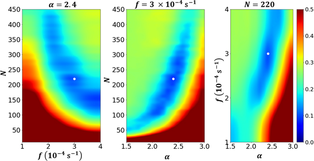
Figure 6. Same as Figure 5, but for Fe xv and intersecting at (2.4, 3 × 10⁻⁴ s−1, 220).
Download figure:
Standard image High-resolution imageThe left panel in each figure clearly shows the trade-off between f and N discussed above. There is an inverse relationship between these quantities, so similar quality fits can be obtained by increasing the nanoflare frequency while decreasing the number of strands.
The center and right panels of each plot show the relation between f or N and the power-law index, α. For a fixed nanoflare frequency f, a larger number of strands implies a larger value of α. Similarly, for a fixed N, a larger f also leads to a greater α. The larger α indicates the nanoflare energy distribution is steeper if there are more strands or a higher nanoflare frequency. This relationship is a consequence of the model needing to reproduce the correct magnitude of the intensity. The values of f and N determine the total number of nanoflares that will occur in each synthetic pixel. Since intensity depends on the total energy release, maintaining the same magnitude of intensity requires that if there are more nanoflares then their average energy must be reduced. Consequently, higher values of f and N lead to steeper power-law distributions.
Figure 7 and 8 illustrate our results for the small N region of parameter space based on the Fe xii and xv intensities, respectively. For Fe xii, the cuts here are through the point (3, 14 × 10−4 s−1, 75) and for Fe xv through (2.8, 12 × 10−4 s−1, 50). In this region of parameter space, we again find the inverse relationship between f and N and the correlation between α and either f or N, which as discussed above, arise due to the relation between the energy input and the intensity. A consequence of this relation is that in this region of parameter space large values of α ≳ 2.5 are required for the nanoflare energy distribution. Power-law indices of that magnitude have been predicted by some models (e.g., López-Fuentes & Klimchuk 2010, 2015).
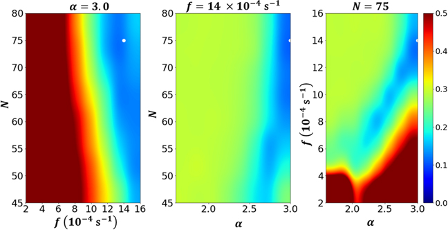
Figure 7. Same as Figure 5 for Fe xii, but for a region of parameter space that allowed for fewer strands with a higher nanoflare frequency per strand. The cuts are intersecting at (3.0, 14 × 10−4 s−1, 75).
Download figure:
Standard image High-resolution image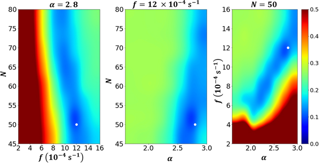
Figure 8. Same as Figure 7, but for Fe xv. The cuts are intersecting at (2.8, 12 × 10−4 s−1, 50).
Download figure:
Standard image High-resolution imageIn general, we find that values of α > 2 are most likely to be consistent with the observations. For small N, we found that α has to be large. For large N, α can be small only if the nanoflare frequency is very low, and even then α > 2 is a better match to the observations (e.g., Figure 5). This is consistent with the basic principle of nanoflare heating models that α > 2 is needed in order that the energy content be dominated by low-energy events (e.g., Hudson 1991; Pauluhn & Solanki 2007). If α were smaller, then there would be high-energy heating events that would be resolved in observations.
It is notable that the regions of parameter space that provide a good fit to the observations using Fe xii overlap with those using Fe xv. This clearly must be the case physically if the heating of each line is due to the same series of nanoflares. However, the observations and comparisons are independent, so the fact that they agree supports that the model is reasonable. Since the emission at different temperatures provides a stronger constraint on the nanoflare parameters, one direction for future work would be to better constrain the parameter space using a comparison that is a composite of intensities from a variety of spectral lines.
Figures 9 and 10 show the results for the single-strand N = 1 case. In this region of parameter space, no tested values of f or α resulted in a reasonable match between the model and the observations. The match improves marginally for high f > 40 s−1 at low α < 2. However, such low values of α are inconsistent with the nanoflare theory as they correspond to an energy distribution that includes many large energy release events and few small ones.

Figure 9. D(α, f, N) comparing a single-strand model to observed intensities for Fe xii.
Download figure:
Standard image High-resolution image
Figure 10. Same as Figure 9, but for Fe xv.
Download figure:
Standard image High-resolution image
These results imply that a single-strand model is inconsistent with nanoflare heating of bright point loops. This makes sense on physical grounds, since in a Parker model the heating is due to reconnection between the various strands making up a multistranded loop, and so multiple strands are a requirement. Conversely, if the loops are heated by nanoflares then they must be composed of many strands. On the other hand if the loops were monolithic, then they could not be heated by nanoflares.
The current results demonstrate some strengths of this model, but other improvements are also possible for future work. One limitation of the current model is the assumption that the nanoflares are independent and occur at random times. In the strand-braiding model of nanoflares, though, the energy release occurs when a threshold level of instability is reached and the magnetic stress that has built up is released. Hence, the nanoflare energy is expected to be proportional to the time interval since the previous nanoflare, or possibly the square of that interval, depending on whether the system relaxes completely or only partially (Cargill 2014). Such physically motivated correlations between the energy distribution and the frequency could be adapted to our method. Doing so would remove some of the redundancy among the parameters. It would also be worthwhile to explore other heating functions that have been studied theoretically and compare those to bright point observations. For example, we have discussed the heating pulse shape and duration as being less important than other parameters, but incorporating these parameters into our modeling would allow us to better quantify how well (or poorly) these factors constrain the space of reasonable nanoflare parameters. Alternative heating functions, such as finite trains of high-frequency nanoflares have been considered by other models and can also be incorporated (e.g., Reep et al. 2013).
A significant issue for nanoflare theory to resolve is understanding the physical meaning of the nanoflare strands. Cartoon illustrations of the concept envision such strands as being magnetic strings braided together to form a rope-like coronal loop, but that picture is likely not literally true. The strands might be a proxy for filamentary density structures that arise due to plasma instabilities. Or, it could be that the strands are a discrete approximation to a continuous distribution of density structuring transverse to the loop. Comparing nanoflare parameters derived from observations interpreted within the strand paradigm with physics-based models will help us to better understand the nature of strands, the structure of coronal loops, and the nanoflare heating process.
5. Conclusions
We have inferred from EIS slot observations the properties of nanoflare heating in a coronal bright point. This approach is inspired by several types of coronal heating studies that have been used for active regions. Our study offers a complementary perspective to those from active region studies. Bright points are relatively simple loop structures, which may more readily allow for a physical understanding of the nanoflare process. Furthermore, for isolated spectral lines, the EIS slot data have a narrow temperature sensitivity, making the interpretation of these observations less ambiguous.
The bright point observations were interpreted using the EBTEL hydrodynamic code in the context of a conventional nanoflare heating process characterized by a power-law energy distribution of index α, average frequency f and N strands in each observed pixel. By comparing the statistical properties of the model and the observed time series of intensities, we identified the region of the parameter space of (α, f, N) consistent with the observations. The details of this region of parameter space are illustrated in Figures 5–8. In general, we find that there is an inverse correlation between f and N, and a direct correlation between α and either f or N. These relations can be explained by the observational constraint that all parameters consistent with the data must input roughly the same average nanoflare heating energy into the bright point. We also found that a single-stranded, N = 1, model was inconsistent with the observations.
There are a number of avenues for refining and extending this work in the future. These include imposing physically motivated relationships among the parameters, exploring the sensitivity to details of the nanoflare heating function, and using the results to understand the physical nature of the postulated strand structures. Additionally, one of the goals of focusing on bright points is to connect nanoflare heating to the magnetic evolution of the loop. By studying a collection of imaging and magnetogram data for bright points, there are prospects for linking nanoflare properties to the magnetic fields that are the underlying source of the heating energy.
This work was supported by NSF Solar Terrestrial Research Program grant AGS1834822 and by NSF Astronomy and Astrophysics grant AST2005887.