


Abstract
The solar wind is a magnetized and turbulent plasma. Its turbulence is often dominated by Alfvénic fluctuations and often deemed as nearly incompressible far away from the Sun, as shown by in situ measurements near 1 au. However, for solar wind closer to the Sun, the plasma β decreases (often lower than unity) while the turbulent Mach number Mt increases (can approach unity, e.g., transonic fluctuations). These conditions could produce significantly more compressible effects, characterized by enhanced density fluctuations, as seen by several space missions. In this paper, a series of 3D MHD simulations of turbulence are carried out to understand the properties of compressible turbulence, particularly the generation of density fluctuations. We find that, over a broad range of parameter space in plasma β, cross helicity, and polytropic index, the turbulent density fluctuations scale linearly as a function of Mt, with the scaling coefficients showing weak dependence on parameters. Furthermore, through detailed spatiotemporal analysis, we show that the density fluctuations are dominated by low-frequency nonlinear structures, rather than compressible MHD eigenwaves. These results could be important for understanding how compressible turbulence contributes to solar wind heating near the Sun.
Export citation and abstract BibTeX RIS
1. Introduction
The solar wind is a high-speed plasma flow emitted from the solar surface, as first predicted by Parker (1958). It was soon discovered that the solar wind is turbulent, containing fluctuations in a vast range of spatial and temporal scales. The free-energy source for solar wind turbulence is typically at large scales, associated with activities near the Sun. (Energy can also be injected by instabilities at kinetic scales driven by beams or temperature anisotropies.) These large-scale perturbations will interact nonlinearly, causing a cascade of energy to smaller scales and forming power-law spectra of magnetic, velocity, and density fluctuations, which are believed to contribute to the solar wind heating.
In the classic picture of solar wind turbulence (see a recent review by Bruno & Carbone 2013), the fluctuations are treated as Alfvénic and incompressible, i.e., the divergence of velocity fluctuations is zero. Theories have been developed to deal with nearly incompressible turbulence in the solar wind, and they have explained many of the key features of solar wind turbulence (Montgomery et al. 1987; Matthaeus & Brown 1988; Matthaeus et al. 1991; Zank & Matthaeus 1992; Zank et al. 2017). However, there exists a non-negligible component of compressible turbulence in the solar wind throughout the heliosphere, characterized by enhanced density fluctuations. Furthermore, there have been several theoretical and numerical studies on compressible MHD turbulence in astrophysical plasmas as well. Radio wave scintillation observations reveal a nearly Kolmogorov spectrum of density fluctuations in the ionized interstellar medium, suggestive of compressible MHD turbulence. Past theory and simulations have suggested that the density fluctuations are due to the slow mode and the entropy mode (Lithwick & Goldreich 2001). Many numerical simulations have been used to understand the nature of compressible MHD turbulence as well (Cho & Lazarian 2003; Kowal et al. 2007; Yang et al. 2017; Shoda et al. 2019; Makwana & Yan 2020). In addition, some previous studies have revealed that, due to different properties of MHD waves, compressible perturbations (associated with fast and slow waves) cascade differently than incompressible perturbations (associated with Alfvén waves). For example, MHD simulations by Cho & Lazarian (2002, 2003) show that fast-mode turbulence tends to form an isotropic spectrum (though fast-mode turbulence seems to be anisotropic in the kinetic regime, as shown by Svidzinski et al. 2009), while Alfvénic turbulence tends to form an anisotropic spectrum with respect to the background magnetic field.
It is worth noting that nonlinear interactions among incompressible and compressible components make the study of compressible turbulence very challenging. In general, the density fluctuations in compressible MHD turbulence can originate from different processes. In the limit of regarding fluctuations as MHD waves, the variations are expected to follow the ω– k dispersion relation of magnetosonic fast and slow modes, and fluctuating density, velocity, and magnetic fields satisfy the relative relation set by eigenvectors in linear theory. In fact, three MHD eigenmodes (fast, slow, and Alfvén modes) can couple with each other nonlinearly through wave–wave interactions (e.g., Chandran 2005). These processes typically render an MHD system with a finite β compressible (where β is the ratio of plasma pressure over the magnetic pressure), even if it starts with incompressible velocity fluctuations. Another way to produce density variations is via instabilities. One example of such processes is the parametric decay instability, where a large amplitude Alfvén wave decays into another Alfvén wave and a slow magnetosonic wave (Derby 1978; Goldstein 1978), which is a source of density fluctuations. This process is of particular relevance to the solar wind near the Sun (Del Zanna et al. 2015; Shi et al. 2017; Fu et al. 2018; Réville et al. 2018; Shoda et al. 2018; Tenerani et al. 2020).
Density fluctuations could, of course, simply arise from the turbulence driving process, then they will continue to cascade to different scales from nonlinear interactions. This process is not necessarily associated with MHD waves. In fact, whether and how much MHD waves exist in turbulence is a nontrivial issue. One approach is to examine whether fluctuations follow the dispersion relation of MHD waves (which is very challenging in general). Here, we use expressions such as waves and nonlinear structures to describe whether fluctuations will follow the eigenmode dispersion relations or not. An example of known nonlinear structures is the pressure-balance structure (PBS; Tu & Marsch 1995; Bruno & Carbone 2013) in the solar wind, where the sum of the magnetic and thermal pressures is nearly constant across the structure. PBS is nonpropagating (though it can be convected by the solar wind) and static, having a zero frequency in the plasma frame. PBS can contain a spatial variation of density, which will be detected as a time series of density fluctuation when the spacecraft is traveling through the solar wind plasma. In principle, the fluctuations in compressible MHD turbulence do not need to satisfy the full dispersion relationships of eigenmodes. Indeed, recent studies of compressible turbulence by Gan et al. (2022) showed that velocity and magnetic fluctuations were dominated by nonlinear structures rather than MHD waves in the simulations using an advanced spatiotemporal 4D fast Fourier transform (FFT) analysis. This conclusion is quite different from many previous analyses where the decomposition of fluctuations is based solely on the spatial variations without their temporal properties (see also Dmitruk & Matthaeus 2009; Andrés et al. 2017; Yang et al. 2019; Brodiano et al. 2021). In this paper, we will also use this 4D FFT approach to examine whether the density fluctuations are associated with MHD waves or nonlinear structures.
One key parameter that controls the compressibility of the turbulence is the turbulent Mach number Mt
, which is the ratio of total velocity fluctuation δ
v to the typical sound speed  (where γ is the polytropic index). Since
  , where β = p/(B2/8π), compressible turbulence is more easily generated in low β plasmas, given a similar level of fluctuation δ
v/vA
(or δ
B/B0 for Alfvénic perturbation). This makes the solar wind close to the Sun especially interesting because β is expected to be lower than unity, compared to about unity at 1 au (Gary 2001). The Parker Solar Probe (PSP) mission is exploring the near-Sun region (Fox et al. 2016), enabling new discoveries and understanding of turbulence in the solar wind (Chen et al. 2020, 2021; Shi et al. 2021). Recently, PSP has entered the sub-Alfvénic region and started to observe turbulence in the low-β solar wind (Kasper et al. 2021).
, where β = p/(B2/8π), compressible turbulence is more easily generated in low β plasmas, given a similar level of fluctuation δ
v/vA
(or δ
B/B0 for Alfvénic perturbation). This makes the solar wind close to the Sun especially interesting because β is expected to be lower than unity, compared to about unity at 1 au (Gary 2001). The Parker Solar Probe (PSP) mission is exploring the near-Sun region (Fox et al. 2016), enabling new discoveries and understanding of turbulence in the solar wind (Chen et al. 2020, 2021; Shi et al. 2021). Recently, PSP has entered the sub-Alfvénic region and started to observe turbulence in the low-β solar wind (Kasper et al. 2021).
There have seen several studies on the relation between density fluctuations δ
ρ and the turbulent Mach number Mt
. Nearly incompressible MHD (NI-MHD) theory (Matthaeus & Brown 1988; Matthaeus et al. 1990; Zank & Matthaeus 1993) predicts  if Mt
is a small parameter, similar to nearly incompressible theory in neutral fluids. Numerical simulations of fluid turbulence have confirmed that the
if Mt
is a small parameter, similar to nearly incompressible theory in neutral fluids. Numerical simulations of fluid turbulence have confirmed that the  scaling holds at small Mt
and it transitions to more complex scaling at large Mt
(e.g., Cerretani & Dmitruk 2019). There was observational evidence in the solar wind that supports Mt
2 scaling and NI-MHD theory (Matthaeus et al. 1991), but other studies found a lack of clear scaling (Tu & Marsch 1994; Bavassano et al. 1995), possibly due to the existence of inhomogeneous structures (Bruno & Carbone 2013). In an inhomogeneous medium NI-MHD theory predicts that the density fluctuations scale linearly with Mt
(Hunana & Zank 2010; Zank et al. 2017; Zank et al. 2021). The density scaling can also depend on β. In a comprehensive study by Cho & Lazarian (2003), by using linear dispersion relations for MHD waves, they concluded that: in low-β plasmas, slow modes give rise to most of the density fluctuations which scale linearly with Mt
; in high-β plasmas, they found that the density fluctuations scale as Mt
2, similar to the NI-MHD limit. Given that PSP is now providing the in situ measurements of compressible turbulence (e.g., Adhikari et al. 2020), we have performed MHD turbulence simulations, particularly with relatively high Mt
, to investigate how various turbulence quantities correlate among themselves.
scaling holds at small Mt
and it transitions to more complex scaling at large Mt
(e.g., Cerretani & Dmitruk 2019). There was observational evidence in the solar wind that supports Mt
2 scaling and NI-MHD theory (Matthaeus et al. 1991), but other studies found a lack of clear scaling (Tu & Marsch 1994; Bavassano et al. 1995), possibly due to the existence of inhomogeneous structures (Bruno & Carbone 2013). In an inhomogeneous medium NI-MHD theory predicts that the density fluctuations scale linearly with Mt
(Hunana & Zank 2010; Zank et al. 2017; Zank et al. 2021). The density scaling can also depend on β. In a comprehensive study by Cho & Lazarian (2003), by using linear dispersion relations for MHD waves, they concluded that: in low-β plasmas, slow modes give rise to most of the density fluctuations which scale linearly with Mt
; in high-β plasmas, they found that the density fluctuations scale as Mt
2, similar to the NI-MHD limit. Given that PSP is now providing the in situ measurements of compressible turbulence (e.g., Adhikari et al. 2020), we have performed MHD turbulence simulations, particularly with relatively high Mt
, to investigate how various turbulence quantities correlate among themselves.
The paper is organized as follows. Section 2 describes the numerical model used in this study. Simulation results and analyses are presented in detail in Section 3. We summarize the main results in Section 4, with the discussion of unresolved issues and possible future directions.
2. Numerical Simulation
To study compressible turbulence and density fluctuations in the context of the solar wind in the inner heliosphere (<1 au), we carry out a series of 3D compressible MHD simulations. We select plasma parameters that represent typical solar wind conditions within 1 au. We use the high-performance code ATHENA++ (Stone et al. 2020) to solve the ideal compressible MHD equations:


with the polytropic equation of state  , where γ is the polytropic index. Since we are interested in local properties of turbulence driven by large-scale free-energy input, our model does not include the global structure of the solar wind. Instead, we assume a system with uniform background magnetic field and periodic boundary conditions. The simulation domain is an elongated box with Lx
= 8π, Ly
= Lz
= 2π and the background magnetic field is B0
e
x
. Periodic boundary conditions are applied in all three directions. The Alfvén crossing time is τA
= Lx
/vA
= 8π. For most of our runs we use 512 cells to resolve each dimension.
, where γ is the polytropic index. Since we are interested in local properties of turbulence driven by large-scale free-energy input, our model does not include the global structure of the solar wind. Instead, we assume a system with uniform background magnetic field and periodic boundary conditions. The simulation domain is an elongated box with Lx
= 8π, Ly
= Lz
= 2π and the background magnetic field is B0
e
x
. Periodic boundary conditions are applied in all three directions. The Alfvén crossing time is τA
= Lx
/vA
= 8π. For most of our runs we use 512 cells to resolve each dimension.
Starting from a quiet uniform plasma (ρ0 = 1, B0 = 1, and zero fluctuations), we perturb the MHD system by adding driving terms in both momentum and magnetic field equations (Equations (2) and (3)). We maintain the divergence-free condition for the magnetic field by keeping ∇ · f b = 0 to machine precision (Gan et al. 2022). For all of the runs, we also keep ∇ · f v = 0 to model incompressible driving at large scales. f v and f b are applied at large scales where their wavenumber k ≤ kinj = 3. By varying the relative strength and phase of f v and f b , we are able to vary the Alfvén ratio rA ≡ ∣δ v ∣2/∣δ B ∣2 and cross helicity σc ≡ (∣ z +∣2 − ∣ z −∣2)/(∣ z +∣2 + ∣ z −∣2) (where z ± ≡ δ v ± δ B are Elsässer variables) of the injected fluctuations. To some degree, they replicate the observed solar wind conditions. By keeping the relative phase and strength of f v and f b and changing the magnitude of both quantities proportionally, we can also vary the driving strength and achieve different levels of turbulence. Typically, an adiabatic equation of state is adopted with γ = 5/3 to simulate MHD turbulence in the solar wind. But we will vary γ and study its effect on compressible turbulence and density fluctuations, as inspired by recent observations from PSP (Nicolaou et al. 2020). γ > 5/3 implies heating of the system by an external energy source (not included in the model), and γ < 5/3 implies cooling.
We should emphasize that, even though we have tried to keep the driving process ∇ · f v = 0, this does not mean that ∇ · (ρ v ) ≈ 0 during the evolution. For example, because we have used f b , the "added" Lorentz force J × B due to injection is typically nonzero. This leads to momentum variations that are not guaranteed to be ∇ · (ρ v ) = 0. Although ∇ · f v = 0 is satisfied through the injection process, the density variations can be excited through the joint injection process of f v and f b . We will discuss this point in more detail in Section 3.
3. Results
The key parameters and turbulent quantities of our MHD simulations are summarized in Table 1. Note that, in addition to these listed runs, we have also performed a few runs with higher resolution (10243) and many lower resolution (2563) runs to map out the parameter space (see below), as well as to check the consistency of the results. In this section, we will first describe the evolution of turbulent quantities under different driving conditions. Second, we present the scaling of density fluctuations as a function of turbulent Mach number Mt and examine how the scaling varies with key plasma/turbulence parameters. Third, we investigate the nature of the density fluctuations and their relation to compressible MHD waves and nonlinear structures.
Table 1. Main Input Parameters (Columns 2–4) and Turbulent Quantities (Columns 5–9) for 3D MHD Simulations
| Run | Number of Cells | β0 | γ | MA | Mt | δ ρ | σc | β |
|---|---|---|---|---|---|---|---|---|
| 1 | 5123 | 1.0 | 1.67 | 0.25 | 0.27 | 0.13 | 0.93 | 1.03 |
| 2 | 5123 | 1.0 | 1.67 | 0.34 | 0.37 | 0.19 | 0.85 | 1.07 |
| 3 | 5123 | 1.0 | 1.67 | 0.17 | 0.19 | 0.09 | 0.91 | 1.01 |
| 4 | 5123 | 0.2 | 1.67 | 0.24 | 0.59 | 0.33 | 0.67 | 0.24 |
| 5 | 5123 | 1.0 | 1.67 | 0.21 | 0.23 | 0.11 | −0.20 | 1.03 |
| 6 | 5123 | 1.0 | 2.7 | 0.28 | 0.24 | 0.10 | 0.93 | 1.08 |
| 7 | 10243 | 1.0 | 1.67 | 0.28 | 0.30 | 0.13 | 0.92 | 1.03 |
| 8 | 2563 | 1.0 | 1.67 | 0.24 | 0.26 | 0.12 | 0.92 | 1.03 |
Note. The system size is 8π × 2π × 2π with a uniform magnetic field B0 = 1 in the x direction. Turbulent quantities are measured in the late stage of each simulation when the system is in a quasi-steady state.
Download table as: ASCIITypeset image
3.1. Evolution of Turbulent Quantities
Our nominal case is Run 1 with an initial β0 = 1 and an adiabatic equation of state (i.e., γ = 5/3). The system is driven by Alfvénic incompressible perturbations at large scales (with kinj = 3) and it has a final cross helicity σc = 0.93. Figure 1(a) shows the time history of the averaged velocity field, magnetic field, and density fluctuations in Run 1, with
where the brackets indicate the rms value over the whole simulation domain. These quantities are measures of the overall level of turbulence. With a continuous energy injection, all three fluctuation quantities increase gradually as a function of time. After an initial growth stage (0 < t < 60), the turbulence reaches a quasi-steady state with a saturated level of fluctuations. Between t = 70 and t = 90, we check the spectra of δ v, δ ρ, and δ B and confirm that they remain nearly unchanged. Since we use an adiabatic equation of state, the total energy of the system is increasing with the continuous injection. After the turbulence is saturated, most of the input energy is converted into the internal energy of plasma, causing plasma heating in the later stage of the simulation (β increases from 1.0 at t = 0 to ∼1.03 at t = 90). Overall, the turbulence and plasma parameters are roughly controlled by the injection.
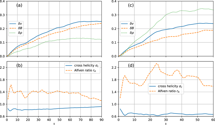
Figure 1. Run 1: β0 = 1.0, (a) time evolution of the magnetic field, velocity field, and density fluctuations. The fluctuation level saturates after about t = 50 when the system enters into a quasi-steady state; (b) time evolution of cross helicity σc , and Alfvén ratio rA . Run 4: β = 0.2, (c–d) Similar to panels (a–b) but for Run 4 with β0 = 0.2.
Download figure:
Standard image High-resolution imageFor Run 1, Mt reaches 0.27 in the quasi-steady state, and δ ρ reaches 0.13. By varying the strength of driving forces ( f b and f v ), we can obtain turbulence with different levels of Mt . In Run 2 (3), which uses the same parameters as Run 1 except for stronger (weaker) driving forces, we obtain a larger (smaller) Mt = 0.37 (Mt = 0.19) and stronger (weaker) density fluctuations δ ρ = 0.19 (δ ρ = 0.09) (see Table 1 for details).
Note that although we keep the injected fluctuations Alfvénic with δ v = δ B, the plasma has the freedom to respond to the injection, and total δ v is slightly larger than δ B throughout the simulation. This can also be seen in Figure 1(b), where rA first increases from 1.2 to 1.6 then reduces to 1.1 (rA = 1 for Alfvénic fluctuations) at the later stage. Similarly, we intend to have an imbalanced turbulence with σc = 0.9, the resulting σc varies from ∼0.8 at the beginning to ∼0.9 at the end of the simulation.
To contrast with Run 1, we carry out Run 4 with the same parameters except for a lower β0 = 0.2. This represents the solar wind condition much closer to the Sun. As shown in Figure 1(c), the fluctuations saturate at t ∼ 40, with a similar level of velocity fluctuation (δ v ∼ 0.24) to Run 1. It is notable that the density fluctuation generated in Run 4 is much higher than in Run 1, with δ ρ ∼ 0.33 (versus 0.13 in Run 1). This is the characteristic response of low-β plasma. Because we hold MA = δ v/vA the same for both runs, Run 4, being lower β, achieves much higher turbulence Mach number Mt with the same δ v. Another feature of Run 4, different from Run 1, is that the Alfvén ratio remains higher than unity (∼1.5 at the later stage, i.e., more energy goes into the velocity fluctuation than the magnetic fluctuation) throughout the simulation, even though the driving forces are Alfvénic. Similarly, the cross helicity remains around 0.7, lower than the value of Run 1. These quantities can be used to study the possible relationship between Alfvénicity and compressibility in the solar wind, too (Bruno & Carbone 2013).
As we emphasized earlier, even though the driving ensures that ∇ · f v = 0 and ∇ · f b = 0, the evolution of both magnetic field (thus Lorentz force) and momentum does not guarantee that ∇ · (ρ v ) = 0. Using Run 1 as an example, Figure 2 depicts the evolution of rms values of various terms in the continuity equation (panel a) along with their probability density functions (PDFs) in panels b-d. (These quantities are calculated using the cell-based values.) It can be seen that, even though ∇ · v ≈ 0 when integrated over volume (i.e., the averaged value is near zero), there are large variances for ∇ · v and ∇ · (δ ρ v ), both of which contribute to large ∇ · (ρ v ) variations. It is also interesting to notice that the ∇ · v term has major contributions throughout the evolution (being dominant in the beginning), the ∇ · (δ ρ v ) term also becomes important as time goes on, even becoming the bigger term after t > 70.
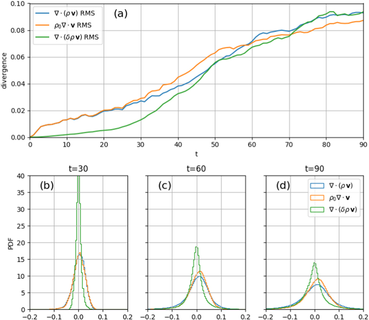
Figure 2. Run 1: (a) History of the rms values of the divergence terms that contribute to the growth of density fluctuations, and histograms of the divergence term PDFs at (b) t = 30, (c) t = 60, and (d) t = 90. In the growing phase of turbulence (t < 60), the total divergence ∇ · (ρ v ) is dominated by the linear term ρ0∇ · v . In the saturation phase, the nonlinear term ∇ · (δ ρ v ) is also quite strong.
Download figure:
Standard image High-resolution image3.2. Scaling of Density Fluctuations
As shown above, the density variations depend strongly on the turbulent Mach number Mt and show some dependence on plasma β and other parameters. To systematically study density fluctuations under various conditions relevant to the solar wind, we explore a large parameter space with different β, σc , γ, and Mt . Before we present our main results, let us first examine the spectral properties of density fluctuations in the nominal case.
Figure 3 shows a surface contour of δ ρ at t = 80 in Run 1. Clearly, δ ρ is anisotropic with much smoother variation along B 0. Although the rms value of δ ρ is 0.13, there are localized structures with density enhancement or depletion with ∣ρ − ρ0∣ > 0.4. The power spectra of δ ρ as a function of k⊥ or k∥ are shown in Figure 4(a). First, we observe that most of the power is contained in the perpendicular direction. It is the same for the power spectra of magnetic field and velocity fluctuations, as shown in Figure 4(a), which is due to the anisotropic cascade of MHD turbulence in magnetized plasmas (Shebalin et al. 1983; Goldreich & Sridhar 1995). Second, the perpendicular spectra have two power-law segments with a break point near k = 100, below which it follows a Kolmogorov law with k−5/3, a signature of the inertial range. The roll-off of the spectra above the break point is due to numerical dissipation at small scales. Third, fluctuations at k ≤ 3 are mainly due to driving applied in the simulation.

Figure 3. 3D snapshot of density fluctuation at t = 80 for Run 1. The density fluctuations are elongated along the direction of the background magnetic field (x), showing strong anisotropy.
Download figure:
Standard image High-resolution image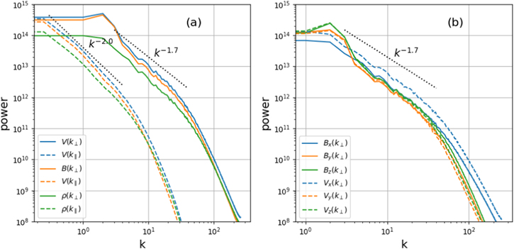
Figure 4. Power spectra of (a) total velocity field, magnetic field, and density field fluctuations and (b) magnetic and velocity field components at t = 80 for Run 1. In the inertial range (3 < k < 40), both the magnetic field and velocity field power spectra follow approximately the Kolmogorov law with  in the perpendicular direction.
Download figure:
Standard image High-resolution imageIn order to study how the density fluctuations will correlate with various quantities, we decide to apply a bandpass to the density power spectra, excluding fluctuations in both the injection range and the dissipation range. This is because the injection region dominates the spectral power, yet its dynamics are subject to driving forces. We can calculate density fluctuations in the inertial range as,

Similarly, we can calculate magnetic field and velocity field fluctuations in the inertial range as  and
and  , respectively. Note that the injection wavenumber kinj is set by the driving forces (kinj = 3 in all our simulations), and the roll-over wavenumber kro is set by the numerical scheme for solving the MHD equations and the resolution of the simulation. With other parameters being the same, Run 7 (10243 cells) has kro ∼ 100, Run 1 (5123 cells) has kro ∼ 40, and Run 8 (2563 cells) has kro ∼ 25. But all three runs yield similar fluctuation levels in the inertial range,
  ,
,  and
and  . They are understandably smaller than the total fluctuations, which include the injection range (cf. Table 1).
Next, we study the relation of density fluctuation  with turbulent Mach number
  (
( ). Due to the limitation of computing resources, we use a large number of low-resolution (2563) simulations to cover the parameter space with β = 0.2, 0.5, 1.0, 2.0, γ = 1.67, 2.70, σc
= 0.0, 0.3, 0.9 and a range of Mt
. The range of each parameter is inspired by observations. For example, PSP observations reported by Nicolaou et al. (2020) suggest that the solar wind protons follow an equation state with a wide range of γ, and the averaged γ increases from 1.7 at 1 au to 2.7 in the inner heliosphere. High σc
and low β are typical for the solar wind close to the Sun (e.g., Kasper et al. 2021), and σc
∼ 0 and β ∼ 1 are typical for the solar wind at 1 au.
). Due to the limitation of computing resources, we use a large number of low-resolution (2563) simulations to cover the parameter space with β = 0.2, 0.5, 1.0, 2.0, γ = 1.67, 2.70, σc
= 0.0, 0.3, 0.9 and a range of Mt
. The range of each parameter is inspired by observations. For example, PSP observations reported by Nicolaou et al. (2020) suggest that the solar wind protons follow an equation state with a wide range of γ, and the averaged γ increases from 1.7 at 1 au to 2.7 in the inner heliosphere. High σc
and low β are typical for the solar wind close to the Sun (e.g., Kasper et al. 2021), and σc
∼ 0 and β ∼ 1 are typical for the solar wind at 1 au.
Figure 5 summarizes results from these low-resolution runs with different combinations of these key parameters. With other parameters (β, σc
, and γ) fixed, we find  scales nearly linearly as a function of
  , i.e.,

The circles are data points extracted from simulations, and the dashed lines are linear fits to each set of runs. Note that although we have some control over σc , it fluctuates in the simulations. So the numbers for σc are not exact, but averaged values. β0 is the initial value of β at t = 0, and β increases slightly in simulation due to heating by injection, as discussed above.
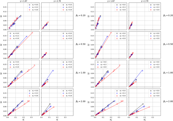
Figure 5. Density fluctuation  as a function of (left) turbulent Mach number
  and (right) Alfvén Mach number
  for a series of 3D low-resolution (2563 cells) MHD simulations with different combinations of parameters β, σ, and γ. Circles are data points extracted from simulations, and dash lines are linear fit to these points.
  scales as
  , and the coefficient C depends weakly on σc
and γ.
, and the coefficient C depends weakly on σc
and γ.
Download figure:
Standard image High-resolution imageSeveral features can be summarized from these results: First, the coefficient C has a relatively weak dependence on β when using  as shown by comparing different rows in Figure 5 (left panel). If we plot the scaling of density as a function of Alfvén Mach number (right panel), there will be strong β dependence, which is not surprising as
  . Second, the dependence of C on both γ and σc
is relatively weak. More balanced turbulence (σc
= 0) yields slightly higher density fluctuations than the imbalanced turbulence (σ = 0.9). This trend is more prominent in runs with higher β values. As we approach the Sun, generally β decreases, γ increases, and σc
increases. Changes in density fluctuation levels can be complicated due to the different effects of these parameters. Interestingly, for the same range of Mt
, density fluctuations near the Sun might be of similar magnitudes as those near 1 au.
. Second, the dependence of C on both γ and σc
is relatively weak. More balanced turbulence (σc
= 0) yields slightly higher density fluctuations than the imbalanced turbulence (σ = 0.9). This trend is more prominent in runs with higher β values. As we approach the Sun, generally β decreases, γ increases, and σc
increases. Changes in density fluctuation levels can be complicated due to the different effects of these parameters. Interestingly, for the same range of Mt
, density fluctuations near the Sun might be of similar magnitudes as those near 1 au.
3.3. Nature of Density Fluctuations
Lastly, we examine the nature of density fluctuations in our simulations. Traditionally, density fluctuations are associated with compressible waves. Among the three linear MHD modes, the Alfvén mode is incompressible, so only fast and slow modes can contribute to density fluctuations. Using linear mode decomposition in the spatial domain, fluctuations can be decomposed into the three MHD modes (Cho & Lazarian 2002). This decomposition is typically done on the velocity field because the velocity fields from the three MHD modes form the bases of a complete orthogonal system. We have performed such decomposition using frames near the end of Run 1. We find that the mode decomposition method gives about 75% of the velocity fluctuation power in the Alfvén mode, about 20% in the slow mode, and less than 5% in the fast mode. The spatial linear mode decomposition approach, however, does not take into account the temporal variations. For example, nonlinear structures, which do not belong to any linear mode, can still be decomposed spatially into three MHD modes. Therefore, as pointed out by Gan et al. (2022), this decomposition may overestimate the contribution from MHD waves.
To better analyze fluctuations in the simulations, we employ 4D FFT analysis (3D for space and 1D for time), in which both spatial and temporal information are used to calculate the Fourier power in the ω– k space (Gan et al. 2022). Using this approach, the power along the dispersion surfaces of MHD waves (numerically we sum over power within 10% of theoretical frequencies) will be regarded as "waves", and fluctuations elsewhere will be called nonwave structures. Figure 6 shows such an analysis of the density fluctuations for Run 1, where we use data from the whole simulation domain in a time window 50 < t < 80 (we exclude the initial growing phase). There is some power in two compressible modes: fast and slow modes. However, it is clear that the majority of the energy resides in the very low-frequency structures, whose frequency is at or near zero and wavenumber is perpendicular to the background magnetic field (referred to as "low-frequency structure" hereafter). This is more clear if we make a 2D cut in the ω − k⊥ plane with k∥ = 0 (panel b). Summing up the power in the low-frequency structure, we find that it comprises nearly 91% of the total power in the simulation box. MHD waves, on the other hand, contribute only a small fraction, less than 9%. Furthermore, the majority of wave power resides in the slow mode (8%), and the power of the fast mode is negligible (<1%), which can also be seen in Panel (c). Similar results were reported by Gan et al. (2022). Finally, Panel (d) shows the anisotropy of the density fluctuation, consistent with Figure 4(a).

Figure 6. (a) Contours of the Fourier power of density fluctuations in the ω– k space using 4D FFT analysis for Run 1, with 50 < t < 80. For visualization purposes, the 4D FFT data has been reduced to 3D by projecting k vector into k⊥–k∥ plane. Gray surfaces represent the dispersion surface of the slow mode (lower) and the fast mode (upper). The majority of the power resides in oblique directions where k⊥ ≫ k∥ (c.f. Figure 4). The fractions of the power carried by the nonlinear structures, slow mode, and fast mode are 91%, 8%, and < 1%, respectively. (b) A 2D cut of the power in the ω–k⊥ plane with k∥ = 0. The white line is the dispersion relation of the fast mode. (c) A 2D cut of the power in the ω–k∥ plane with k⊥ = 5. The upper white line is the dispersion relation curve of the fast mode, and the lower white line is the dispersion relation curve of the slow mode. Most of the wave power is in the slow mode. (d) Fourier power of fluctuations in the k⊥–k∥ plane, showing strong anisotropy in the perpendicular direction.
Download figure:
Standard image High-resolution imageUsing 4D FFT analysis of the density fluctuations in the low-β Run 4, we obtain qualitatively similar results. As in Figures 7(a) and (c), the dispersion surface/curve of the slow mode ( ) is lower with a lower β. Still, the nonlinear structures contribute 97% of the total power, slow mode contributes 3%, and fast mode is negligible.
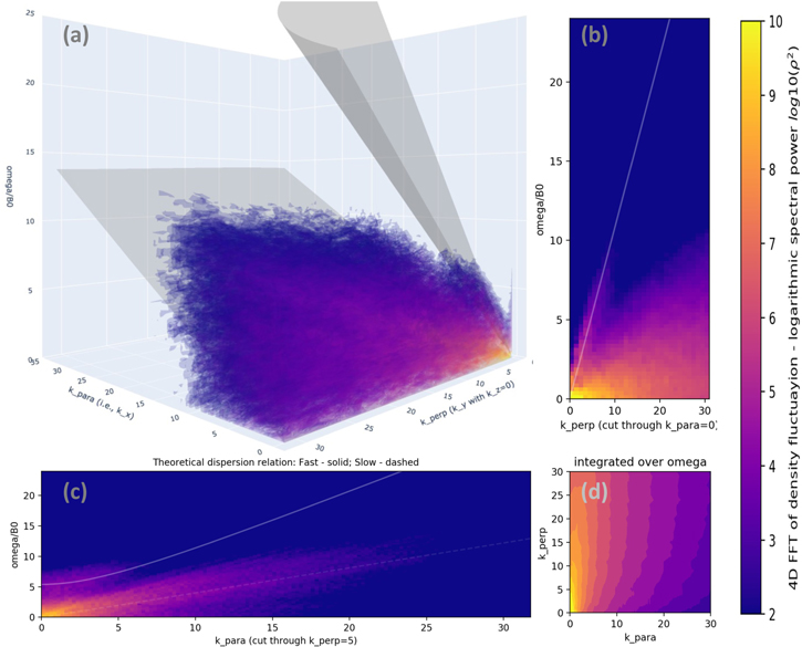
Figure 7. 4D FFT analysis of density fluctuations in Run 4, with t < 60. 97% of the power is in the nonlinear structures, and 3% is in the slow mode. The contribution from the fast mode is negligible. The format is the same as in Figure 6.
Download figure:
Standard image High-resolution image4. Conclusion and Discussion
In this paper, using a large set of 3D MHD simulations, we investigate the development and properties of compressible turbulence driven by continuous large-scale perturbations. We have found:
- 1.Although the driving (at large scales) is maintained incompressible throughout the simulations, compressible fluctuations of varying magnitudes can still be generated via driving, and they can be monitored via the rms values of ρ, ∇ · v , and ∇ · (δ ρ v ). In principle, compressible fluctuations can be generated via wave–wave interaction or mode conversion in an MHD system, and it is likely that some of these processes are occurring (particularly for low β simulations), but we believe that the density fluctuations in our simulations are primarily due to driving, which is enforced in both the momentum and magnetic fields. The turbulent Mach number in our simulations ranges from a few percent to the order of unity (including the driving range). After removing fluctuations in the driving range, the turbulent Mach number drops down to be less than 0.3.
- 2.Simulations show a linear scaling of density fluctuation in the inertial range as a function of turbulence Mach number
 , where the coefficient C depends weakly on σc
and γ.
, where the coefficient C depends weakly on σc
and γ. - 3.Density fluctuations are dominantly caused by nonlinear structures with very low-frequency and large k⊥. The nonlinear structures contribute to more than 90% of the fluctuation based on the 4D FFT analysis whereas the actual compressible MHD waves contribute to a few percent in total power. These nonlinear structures could be mistakenly attributed to MHD modes when using the mode decomposition method based on the spatial variations alone. The contribution from the fast modes is negligible.

We have obtained a linear scaling of the density fluctuation as a function of turbulent Mach number based on our 3D MHD simulations. This is different from the prediction of nearly incompressible MHD theory (Matthaeus & Brown 1988; Zank & Matthaeus 1992), i.e.,  . The discrepancy may be caused by several reasons. First of all, NI-MHD theory assumes Mt
≪ 1, whereas in our simulations Mt
ranges between 0.1 − 0.9 (including the injection range). Second, NI-MHD theory attributes the density fluctuations to pseudo-sound, which is a zero-frequency structure with ∇ ·
v
≈ 0. As shown in our simulations, there are non-negligible ∇ ·
v
fluctuations, and the frequency of these nonlinear structures is low but not zero. The scaling of density fluctuation was also compared with NI-MHD theory using solar wind data (Matthaeus et al. 1991; Klein et al. 1993; Tu & Marsch 1994; Bavassano et al. 1995), but the spreads in both Mt
and δ
ρ data points were too large to draw any firm conclusions. Note that, in situ observation is 1D sampling through the solar wind turbulence, and the statistical properties are sensitive to sampling conditions such as the angle between the sampling line and the background magnetic field. They may also depend on plasma and turbulence parameters such as σc
and γ, as suggested by the simulations. Our linear scaling can be tested by observations if observational data can be grouped further by these parameters. Furthermore, how these results could vary depending on the driving processes needs to be further investigated (Gan et al.2022).
. The discrepancy may be caused by several reasons. First of all, NI-MHD theory assumes Mt
≪ 1, whereas in our simulations Mt
ranges between 0.1 − 0.9 (including the injection range). Second, NI-MHD theory attributes the density fluctuations to pseudo-sound, which is a zero-frequency structure with ∇ ·
v
≈ 0. As shown in our simulations, there are non-negligible ∇ ·
v
fluctuations, and the frequency of these nonlinear structures is low but not zero. The scaling of density fluctuation was also compared with NI-MHD theory using solar wind data (Matthaeus et al. 1991; Klein et al. 1993; Tu & Marsch 1994; Bavassano et al. 1995), but the spreads in both Mt
and δ
ρ data points were too large to draw any firm conclusions. Note that, in situ observation is 1D sampling through the solar wind turbulence, and the statistical properties are sensitive to sampling conditions such as the angle between the sampling line and the background magnetic field. They may also depend on plasma and turbulence parameters such as σc
and γ, as suggested by the simulations. Our linear scaling can be tested by observations if observational data can be grouped further by these parameters. Furthermore, how these results could vary depending on the driving processes needs to be further investigated (Gan et al.2022).
Finally, we have identified that the majority of the density fluctuations come from nonlinear structures that do not follow the dispersion relation of linear MHD waves, based on 4D Fourier analysis. However, the exact nature of the structures and their generation mechanism are not fully understood. How these structures are related to the pressure-balance structures (Vasquez & Hollweg 1999), critically balanced structures (Goldreich & Sridhar 1995), pseudo-sound structures (Matthaeus et al. 1990), or entropic fluctuations (Zank et al. 2021) remains to be investigated. We leave these topics to future investigation.
The research was supported by NASA under Award No. 80NSSC20K0377. The Los Alamos portion of this research was performed under the auspices of the U.S. Department of Energy. We are grateful for support from the LANL/LDRD program and DOE/OFES. Computing resources were provided by the Los Alamos National Laboratory Institutional Computing Program, which is supported by the U.S. Department of Energy National Nuclear Security Administration under Contract No. 89233218CNA000001. We thank Professor William Matthaeus for helpful discussions and Professor Gary Zank for valuable inputs.
Software: Athena++ (Stone et al. 2020), Matplotlib (Hunter 2007).