


Abstract
The relationship between the continuum intensities and magnetic fields for stable and decaying sunspots is analyzed using the scattered-light-corrected data from the Helioseismic and Magnetic Imager. From our analysis, the main differences between stable and decaying sunspots are as follows. In the continuum intensity range from 0.35Iqs to 0.65Iqs, where Iqs is the continuum intensity of the quiet solar surface, the relationship between continuum intensity and transverse magnetic field and the relationship between continuum intensity and inclination display a much higher scatter during the decaying phase of the sunspots. During and after the formation of the light bridge, the scatter plots show a bifurcation that indicates that the two umbrae separated by the light bridge have different thermodynamic properties. The continuum intensity of the umbra in a decaying sunspot is brighter than that of the stable sunspot, indicating that the temperatures in the umbra of decaying sunspots are higher. Furthermore, our results show that the mean continuum intensity of the umbra gradually increases during the decay of the sunspot, but the mean continuum intensity of the penumbra remains constant. Simultaneously, the vertical and transverse magnetic field strengths in the umbra gradually decrease, and the vertical magnetic field strengths in the penumbra gradually increase. The changes in the umbra occur earlier than the changes in the penumbra of the decaying sunspot, suggesting that the umbral and penumbral decay may be an interdependent process during the decay of the sunspot.
Export citation and abstract BibTeX RIS

Original content from this work may be used under the terms of the Creative Commons Attribution 4.0 licence. Any further distribution of this work must maintain attribution to the author(s) and the title of the work, journal citation and DOI.
1. Introduction
The relationship between magnetic field strength (B) and continuum intensity (Ic ) in a sunspot is one important topic in solar physics. Understanding this relationship will give some insights into the energy transport of sunspots, as well as the fundamental physical processes that occur in sunspots. Early investigations focused on theoretical explanations for the umbra of a sunspot (Dicke 1970; Cowling 1976; Maltby 1977). Since the continuum intensity of the sunspot can be converted into the continuum temperature (T) by assuming that the observed intensity satisfies Planck's function (Martinez Pillet & Vazquez 1990), the relations between B and Ic (or T) within the umbra (Martinez Pillet & Vazquez 1993) and whole sunspot (Kopp & Rabin 1992; Balthasar & Schmidt 1993; Solanki et al. 1993; Stanchfield et al. 1997; Westendorp Plaza et al. 2001; Mathew et al. 2004; Tiwari et al. 2015) have been extensively studied. Many studies indicate that the B of a sunspot has a negative relationship with its Ic (or T; Norton & Gilman 2004). The lowest value of Ic (or T) inside the sunspot umbrae always corresponds to the largest magnetic field strength. However, the details of this relationship in the whole sunspot are still subject to some debate (Solanki 2003; Jaeggli et al. 2012; Tiwari et al. 2015; Valio et al. 2020).
The relationship of B with Ic (or T) in the whole sunspot shows pronounced differences between the umbra and penumbra and has a complex nonlinear relationship (Stanchfield et al. 1997; Mathew et al. 2004; Tiwari et al. 2015). There are three typical features: (1) a darkest part of the umbra with a sharp increase in magnetic field strength at relatively constant continuum intensity (or temperature), (2) an umbra–penumbra transition with a small decrease of magnetic field strength in a relatively wide range of continuum intensity (or temperature), and (3) a penumbral part with a nearly constant continuum intensity (or temperature) for a wide range of magnetic field strength (Stanchfield et al. 1997; Westendorp Plaza et al. 2001; Mathew et al. 2004; Watson et al. 2014; Tiwari et al. 2015; Sobotka & Rezaei 2017).
In particular, Jaeggli et al. (2012) analyzed the relationship between Ic and B (Ic –B) in seven sunspots and proposed that an abundance of molecular hydrogen (H2) in the umbra may cause the rapid increase in magnetic field strength at relatively constant temperature. The formation of H2 can reduce the gas pressure in the umbral atmosphere without a change in the temperature, which may lead to a large change in the umbral magnetic field strength. Further analyses of Jaeggli et al. (2012) suggested that the relation at different evolution stages is different. The differences of the Ic –B relation in the formation and decay phases of the sunspot have already been reported by Leonard & Choudhary (2008). Leonard & Choudhary (2008) found that the Ic –B slope decreases for old sunspots. However, the difference in the Ic –B relationship during the decay of sunspots has not been explained.
The decay phase of sunspots can last from a few days to several months. The decay process of sunspots has been widely studied (e.g., Petrovay & Moreno-Insertis 1997; Martínez Pillet 2002; Deng et al. 2007; Litvinenko & Wheatland 2015; Imada et al. 2020; Muraközy 2020). The sunspot decay is mainly manifested by the disappearance of a penumbra, the reduction of area and magnetic flux, and the appearance of moving magnetic features (Romano et al. 2020). It is unclear what changes occur in the magnetic field parameters during decay. Observations suggest that the horizontal magnetic field of the penumbra would gradually rise and become vertical at the initial stage of sunspot decay (Bellot Rubio et al. 2008; Watanabe et al. 2014; Verma et al. 2018). As a result, the penumbra of the decaying sunspot would disappear in the photosphere. In contrast to the observations, simulations suggest that the submergence of horizontal magnetic field is a dominant process in the sunspot decay (Rempel 2015). The change in the horizontal magnetic field during the sunspot decay needs to be further studied.
The relationship between continuum intensity and the magnetic field has significant consequences for energy transport in the sunspot (Borrero & Ichimoto 2011). A detailed study of the relationship of continuum intensities with the magnetic fields in different evolution phases would help us to better understand the decay process of the sunspot. Actually, little work has been specifically directed at the dependence of the continuum intensity on the magnetic field at different evolutionary phases of sunspots.
In this paper, we have selected a sample consisting of five stable and five decaying sunspots and then analyzed the relations between the continuum intensities and the magnetic fields in these sunspots. The target of this work is to shed some light on the mechanisms of sunspot decay by comparing these relations between stable and decaying sunspots. The paper is organized as follows. The observations are described in Section 2. The analysis of the data is presented in Section 3. Finally, the conclusions and discussions are described in Section 4.
2. Data Selection and Correction
Ten sunspots (five stable and five decaying) are selected based on the following conditions: (1) they have α magnetic configurations and poor-flare activities, (2) there are no large flares (M- or X-type flares), and (3) they are located close to the solar disk center (μ > 0.86). The μ is defined as  , where θ is the angle between the line of sight (LOS) and the surface normal.
Under the above criteria, the stable sunspots are NOAA Active Regions 12600, 12079, 12375, 12513, and 12533. The decaying sunspots are NOAA ARs 12662, 12097, 12170, 12477, and 12680. Among them, as examples, we analyze the dynamics of a stable sunspot in NOAA AR 12600 and a decaying sunspot in NOAA AR 12662. The stable sunspot of NOAA AR 12600 and decaying sunspots of NOAA AR 12662 are investigated during the periods from 12:00 UT on 2016 October 10 to 20:00 UT on 2016 October 14 and from 00:00 UT on 2017 June 17 to 08:00 UT on 2017 June 17, respectively.
The data are obtained from the Helioseismic and Magnetic Imager (HMI; Schou et al. 2012a; Scherrer et al. 2012b) on the Solar Dynamics Observatory (SDO; Pesnell et al. 2012). HMI provides the full-Sun-averaged I, Q, U, V images at six wavelengths in the Fe i 617.3 nm absorption line. The continuum full-disk images of HMI are retrieved from the right and left circular polarization at each wavelength with a spatial scale of about 0 5 pixel–1 and a cadence of 45 s. Stokes parameters are obtained through the polarization information observed within 12 minutes and then are inverted using the Very Fast Inversion of the Stokes Vector code (Borrero et al. 2011; Bobra et al. 2014; Centeno et al. 2014; Hoeksema et al. 2014), which assumes a Milne–Eddington model of the solar atmosphere. The 180° azimuthal ambiguity in the transverse magnetic field is resolved by the minimum energy algorithm (Metcalf et al. 2006; Leka et al. 2009).
Because of the effect of stray light on photometric studies (Mathew et al. 2007; Criscuoli & Ermolli 2008; Yeo et al. 2014), it is necessary to calibrate the stray-light contamination. For darker sunspots, their intensity observations can be significantly influenced by the stray light from the much brighter surroundings. As a result, the observed images are actually the convolution of a real image with the point-spread function (PSF) of the instrument. Therefore, a deconvolution of the observed image with the HMI's PSF could diminish the influence of stray light to improve the quality of the HMI images. Couvidat et al. (2016) provided a modeled PSF to correct the scattered light of HMI data in detail. The PSF is an Airy function convolved with a Lorentzian. More detailed information on the PSF of HMI can be found in Wachter et al. (2012), Couvidat et al. (2016), and Criscuoli et al. (2017). The deconvolution of this PSF on the intensity images and the averaged Stokes profile data of HMI can be corrected for stray light to obtain the deconvolved HMI maps.
The deconvolution results can be found in JSOC with names similar to the original but with the qualifying term "_dconS" appended. Our analysis was performed with the deconvolved HMI maps, and the data series used are hmi.B_720s_dconS and hmi.Ic_720s_dconS. These data sets are processed at a cadence of every 1 hr. Notably, the sunspots are studied by using the corrected data and the HMI maps, which we refer to as the HMI deconvolved maps.
To obtain vector magnetic field, we used four segments: total magnetic field, inclination, azimuth, and disambiguated to generate Br , Bθ , Bφ by using a cylindrical equal area (CEA) projection. The transformation of the vector magnetic field into CEA maps was performed with a code modified from Xudong Sun's sswidl routine bvec2cea.pro (Sun 2013). The field components (Br , Bθ , Bφ ) are identical to the heliographic components (Bz , − By , Bx ) in Gary & Hagyard (1990). The total magnetic field strength (B), vertical magnetic field strength (Bz ), transverse magnetic field strength (Bt ), and magnetic inclination angle (γ) are computed by using the data in CEA coordinates.
We identify the inner and outer boundaries of sunspots in order to obtain different physical parameters in different parts of the sunspot. For this purpose, we normalized all the continuum intensity images by the local quiet-Sun continuum intensity (Iqs), where Iqs is the average quiet-Sun continuum intensity close to the sunspot. The edge of the umbra is defined by the normalized intensity (Ic = I/Iqs) of 0.6. The region of the sunspot umbra is defined as the area with its intensity smaller than 0.6Iqs. The contour with a level of 0.9 in normalized intensity corresponds to the outer boundary of the sunspot penumbra.
Figure 1 shows the original HMI maps, the deconvolved HMI maps, and the scatter plots of the values of the original versus deconvolved data. The top row shows the difference of continuum intensity maps of a decaying sunspot before and after applying the scattered-light correction. The bottom row is similar, but for the vertical magnetic field (Bz ) data. The white contours indicate the boundaries of the sunspot as seen in the original continuum intensity maps. Figures 1(a3) and (b3) show the results of original data versus the deconvolved data in the same frame. The blue circles mark the data of the sunspot. The deconvolved continuum images exhibit a higher granular intensity contrast and a lower minimum umbral intensity. The Bz values are stronger after applying the scattered-light correction, especially in the plage and umbral regions. The uncorrected field strength values are low owing to the scattered light with a low polarization signal from the quiet Sun. The comparison of total magnetic field (B), transverse magnetic field (Bt ), and magnetic inclination angle (γ) data before and after stray-light calibration can be found in the Appendix.
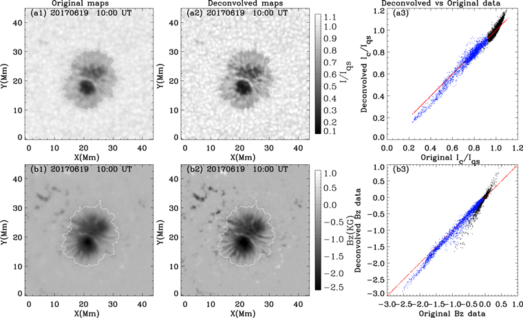
Figure 1. Comparison of the original HMI maps with deconvolved ones for the sunspot on NOAA AR 12662 observed on 2017 June 19 10:00 UT. The top row shows the difference of continuum intensity maps before and after applying the scattered-light correction. The white contours indicate the boundaries of the sunspot as seen in the original continuum intensity maps. The bottom row is similar, but for the vertical magnetic field (Bz ) data. The third column shows the results of original data vs. the deconvolved data in the entire frames of the first and second columns. The blue circles mark the data of the sunspots.
Download figure:
Standard image High-resolution imageWhen the sunspots are far from the disk center, the magnetic contours of the sunspots will shift relative to the intensity contours (Schmassmann et al. 2018). Schmassmann et al. (2018) calculated this shift and found that the boundary of the umbra and penumbra would shift 1.3 pixels in the solar limb. The projection effects are negligible in our study because the observed sunspots are located close to the disk center. The heliocentric angle of the centroid of the studied sunspots is smaller than 30°.
3. Results
3.1. Relations of Ic with B, Bz , Bt , and γ for Sunspots in NOAA ARs 12600 and 12662
We investigate the evolution of the stable sunspot in NOAA AR 12600 and a decaying sunspot in NOAA AR 12662 and analyze the relations of Ic with B, Bz , Bt , and γ. Figures 2(a1)–(a5) and (b1)–(b5) display the evolution of the stable sunspot of NOAA AR 12600 and the decaying sunspot of NOAA AR 12662 for 5 days in the continuum intensity images. The μ in Figure 2 shows the values of μ in the umbral center at a selected time. The white and black contours represent the inner (Ic = 0.6) and outer (Ic = 0.9) boundaries of the sunspots as seen in the continuum intensity.
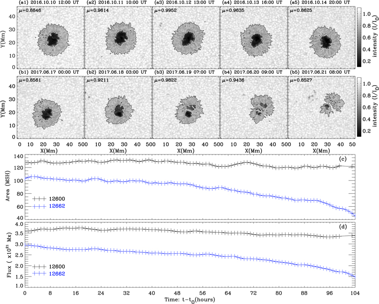
Figure 2. (a1–a5) Continuum intensity images of the stable sunspot in NOAA AR 12600 acquired by SDO/HMI. (b1–b5) Continuum intensity images of the decaying sunspot in NOAA AR 12662. The white and black contours represent the inner (Ic = 0.6) and outer (Ic = 0.9) boundaries of the sunspots as seen in the continuum intensity. The letter μ shows the values of μ in the umbral center at the times given in each panel. (c) Change in area contained within the sunspot boundary (containing the penumbra and umbra). (d) Change in the magnetic flux contained within the penumbra and umbra. The black and blue curves indicate the parameter variations of the sunspots in NOAA ARs 12600 and 12662, respectively.
Download figure:
Standard image High-resolution imageThe morphologies of the two sunspots are very similar in the initial stage. The two sunspots are relatively symmetric with the fully annular penumbra (see the first column of Figure 2). The stable sunspot kept its shape for several days (from 2016 October 10 to 14; see Figures 2(a1)–(a5)). In addition, the area and total magnetic flux of this sunspot, computed in the region of the black contours of Figures 2(a1)–(a5), show little changes during the considered observational time. The results indicate that the sunspot of NOAA AR 12600 is in a stable phase (see the black curves of Figures 2(c)–(d)).
For the sunspot in NOAA AR 12662, a light bridge appears in the middle of the sunspot on 2017 June 19, indicating the onset of its decay. From 2017 June 19 to 21, the decaying sunspot gradually loses its penumbra. The symmetric morphology of the decaying sunspot is completely destroyed at 10:00 UT on 2017 June 21 (see Figures 2(b1)–(b5)). The area and total magnetic flux of the whole decaying sunspot, computed in the region of the black contours of Figures 2(b1)–(b5), show monotonic decrease during the observational period considered. The decaying sunspot decreases its area from 100 to 45 MSH and its magnetic flux from 2.8 × 10²¹ Mx to roughly 1.4 × 10²¹ Mx (see the blue curves of Figures 2(c)–(d)). These results confirm that the sunspot of NOAA AR 12662 is in a decaying phase.
Figures 3(a1)–(a5) show the scatter plots of Ic and B for all spatial points within the stable sunspot. The boundary of sunspot umbra and penumbra is defined as the threshold of Ic = 0.6, as shown by the red vertical dashed lines in each panel. The black points denote the umbral values, and the gray points represent the penumbral values.
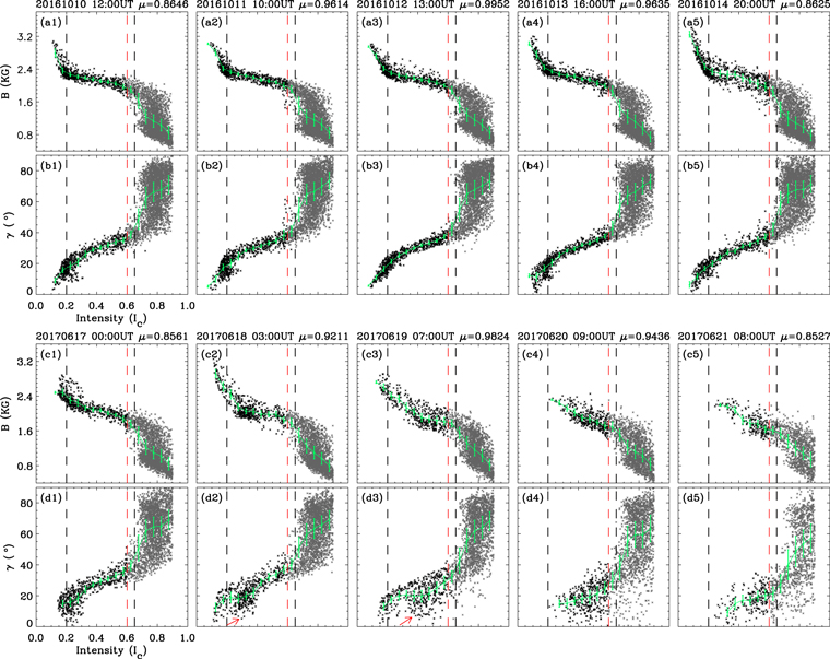
Figure 3. Scatter plots of Ic and B for all spatial points within the stable sunspot (panels (a1)–(a5)) and the decaying sunspot (panels (c1)–(c5)), and scatter plots of Ic and γ for all spatial points within the stable sunspot (panels (b1)–(b5)) and the decaying sunspot (panels (d1)–(d5)). The black vertical dashed lines indicate the continuum intensity corresponding to Ic = 0.2 and Ic = 0.65. The red vertical dashed lines indicate the inner boundary of sunspot, Ic = 0.6. The black and gray points denote the umbral and penumbral values, respectively. The green curves represent the mean and standard deviation of the magnetic field values for each Ic = 0.05 interval between 0.1 and 0.9, where the error bar represents the standard deviation.
Download figure:
Standard image High-resolution imageThe Ic –B relationship of the stable sunspot exhibits a nonlinear anticorrelation, liking a tilted letter "S." This result is qualitatively similar to the results obtained by earlier investigations (e.g., Stanchfield et al. 1997; Mathew et al. 2004; Jaeggli et al. 2012; Tiwari et al. 2015). In the stable sunspot umbra (black points), B decreases with the increase of Ic . The Ic –B relationship in the umbra can be separated into two regions. When Ic < 0.2, the slope of B versus Ic changes obviously. In the interval of Ic < 0.2, the B decreases sharply with the increase of Ic . When Ic > 0.2, the B decreases slowly with the increase of Ic . A possible reason for the sharp change of field strength within a small range of continuum intensity was discussed by Jaeggli et al. (2012). They proposed that the formation of H2 in the umbra can reduce the gas pressure in the umbral atmosphere without a change in the temperature, which may lead to a large change in the umbral magnetic field strength. For the stable sunspot penumbra (gray points), the Ic –B plots can be divided into two regions: a region of lower continuum intensity (Ic < 0.65) and another region of higher continuum intensity (Ic > 0.65). The B decreases slowly with the increase of Ic in the region of Ic < 0.65 and decreases rapidly with the increase of Ic in the interval of Ic > 0.65.
For the stable sunspot, the Ic –B relationship can be roughly divided into three intervals: Ic < 0.2, 0.2 < Ic < 0.65, and Ic > 0.65. The interval of Ic < 0.2 is the central region of the umbra. The B decreases sharply with a little increase of Ic in this interval. The 0.2 < Ic < 0.65 interval is an umbra–penumbra transition region. The B gradually decreases with the increase of Ic from 0.2 to 0.65. The third interval (Ic > 0.65) is mainly located in the outer penumbra. In this interval, the B rapidly decreases with Ic , and the same Ic value corresponds to multiple B.
In order to quantify the divergence in the scatter plots, we used δ Ic = 0.05 as the segmentation unit, divided the range of Ic from 0.1 to 0.9 into 16 intervals, and then calculated the mean value and standard deviation of magnetic field within each interval. The results are shown with the green curves, where the error bar represents the standard deviation of each interval. By comparing the errors of the umbra and penumbra regions, the standard deviation of the penumbra region is relatively large, which means that the scatter of the Ic –B relationship in the penumbra region is relatively large. This large scatter of the penumbra is determined by the fine structure (bright and dark filaments) and interlocking-comb magnetic structure (spines and intraspines) of the penumbra (Borrero & Ichimoto 2011).
Furthermore, it is worth noting that the Ic –B relationship changes very little during the evolution of the stable sunspot. The ranges of intensity and total magnetic field strength are almost unchanged. It is noteworthy that the Ic –B relationship is influenced by sunspot position on the solar disk (Leonard & Choudhary 2008). Carefully comparing Figures 3(a1)–(a5), it can be found that the points of the Ic –B relationship at the center of the solar disk are more concentrated. The standard deviations of the Ic –B relationship in the intervals of 0.2 < Ic < 0.65 are greater; see Figure 3(a5). When the sunspot is located away from the disk center, the inferred Bz would be underestimated (the observational values are smaller than the real local values). We observe higher layers as we approach the limb, and the magnetic field is weaker at higher layers because the magnetic field decreases with height. As a result, the Ic –B relationship will shift integrally to smaller magnetic field strength. However, as shown in Figure 3(a5), only a small portion of the points are shifted. Thus, the shift of points in the plot is not merely due to the measurement errors. The scatter of the plots varies a little, which is shown as the variation of the standard deviation (the error bar) in each interval being relatively small (as for the green curves shown in Figures 3(a1)–(a5)). This result implies that B is highly correlated with Ic in the stable sunspot.
Figures 3(b1)–(b5) show the relationship of Ic and γ for the stable sunspot. The Ic − γ displays a nonlinear shape. The value of γ in the umbra is below ∼40°. In the higher continuum intensity (Ic > 0.65) region, a steep increase in γ with the increase of Ic is found. The results are consistent with the fact that the penumbral magnetic field is inclined. For the stable sunspot, the aspects of the Ic − γ relationship are roughly similar during its evolution.
Figures 3(c1)–(c5) present the temporal evolution of the Ic –B relationship for the decaying sunspot. At first glance, the plots of the decaying sunspot are very different from the stable ones, mainly in the umbra. The slope change of the B − Ic in the decaying sunspot umbra is not observed. However, in the penumbra (0.6 < Ic < 0.9), the frame of the B − Ic appears similar to the stable sunspot without much change. The variation of the error bar in each interval is not significant. This result implies that the change in B over time is very well correlated with the change in Ic over time.
Figures 3(d1)–(d5) show the temporal evolution of the Ic − γ relationship for the decaying sunspot. The scatter plots of the decaying sunspot are more scattered than those of the stable sunspot. For the stable sunspot, the pixels with small γ ( < 20°) are mainly concentrated in the darker region (Ic < 0.2). In contrast, the decaying sunspot has more brighter pixels in the range of γ < 20°. Moreover, the scatter of the Ic − γ relation is increased gradually during the decay of the sunspot. As an example, taking the Ic interval of 0.6–0.65, its standard deviation gradually increases from around 6° at 00:00 UT on 2017 June 17 to 11° at 09:00 UT on 2017 June 20. Initially, this change is more pronounced in the umbra−penumbra transition region (0.2 < Ic < 0.65). The appearance of the brighter pixels with small γ causes the Ic − γ relation in the umbra to show a bifurcation (indicated by the arrows).
Figures 4(a1)–(a5) show the scatter plots of Ic and the vertical magnetic field strength (Bz ) for all spatial points within the stable sunspot. The Ic –Bz relation presents a similar trend to the Ic –B relation, except that Bz slowly decreases to zero at the highest continuum intensity. As shown in Figures 4(a1)–(a5), it is noticeable that the Ic –Bz relation remains similar during the evolution of the stable sunspot and the variations of the standard deviation in each interval are very small.
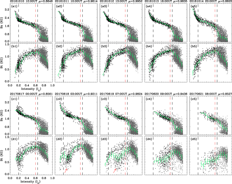
Figure 4. Scatter plots of Ic and Bz for all spatial points within the stable sunspot (panels (a1)–(a5)) and within the decaying sunspot (panels (c1)–(c5)), and scatter plots of Ic and Bt for all spatial points within the stable sunspot (panels (b1)–(b5)) and within the decaying sunspot (panels (d1)–(d5)). The vertical dashed lines and symbols have the same meaning as in Figure 3.
Download figure:
Standard image High-resolution imageFigures 4(b1)–(b5) show the relationship between the Ic and the transverse magnetic field strength (Bt ) for the stable sunspot. As shown in Figures 4(b1)–(b5), Bt increases with the increase of Ic below Ic = 0.65. When Ic is below 0.2, the Ic –Bt shows a steep increase with the increase of Ic . Toward the higher continuum intensity (Ic > 0.65), Bt gradually decreases with the increasing Ic . This result differs slightly from the study of Mathew et al. (2004), who found that Bt increases over the whole intensity (see Figure 2 of Mathew et al. 2004). During the evolution of the stable sunspot, the Ic –Bt relationship remains a similar profile and the maximum and minimum values of Bt are almost unchanged.
Figures 4(c1)–(c5) show the temporal evolution of the Ic –Bz relationship for the decaying sunspot. The Ic –Bz plots of the decaying sunspot are very similar to those of the stable sunspot at first, slightly shifted to higher continuum intensity. With the decay of the sunspot, the maximum value of Bz gradually decreases.
Figures 4(d1)–(d5) show the temporal evolutions of the Ic –Bt relationship for the decaying sunspot. The Ic –Bt relationship in the decaying sunspot shows higher scatter, especially in the darker continuum intensity region (Ic < 0.65). For example, in the interval of 0.6 < Ic < 0.65, its standard deviations of Bt values gradually increased from ∼100 G at 00:00 UT on 2017 June 17 to ∼270 G at 09:00 UT on 2017 June 20. During the decay of the sunspot, the maximum value of Bt gradually decreases. It is obvious that a bifurcation appears in the Ic –Bt relationship during the decay of the sunspot, which is similar to the Ic − γ relationship. The number of pixels in the sunspot with brighter (Ic > 0.6) and smaller transverse field (Bt < 500 G) increases.
The differences between the stable and the decaying sunspots in the relationship between the continuum intensity and the components of the magnetic field vector can be summarized as follows: (1) The brighter pixels are more numerous in the umbra region of the decaying sunspot. (2) The degree of scattering is greater in all relationships of the decaying sunspot, and the scatter increases with the decay of the sunspot, especially in the plots of Ic − γ and Ic –Bt . In the Ic –Bt relationship of the decaying sunspot, the standard deviation increased 2.7 times in the interval of 0.6 < Ic < 0.65 over about 3 days. (3) The plots of Ic − γ and Ic –Bt show obvious bifurcation in the umbral region at the beginning of sunspot decay, and the changes of γ and Bt are similar during the decay phase. We guess that the bifurcation of the Ic − γ relationship may be caused by the influence of Bt , although other reasons cannot be ruled out. In the following discussion of the bifurcation, we mainly depicted the bifurcation structure in the plots of Ic –Bt .
For the decaying sunspot, the branches in the plots of the Ic –Bt relationship are related to the light bridge that appears in the umbra. Figures 5(a1)–(a4) show the decay process of the sunspot with the formation of a light bridge. The light bridge forms as a result of an intrusion of bright filaments from the boundary of the umbra and penumbra. As the filaments gradually progress deeper into the umbra, a light bridge appears. Subsequently, the light bridge fragments the sunspot umbra into two umbral cores: a darker core and a brighter core.
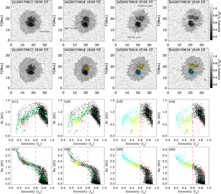
Figure 5. (a1–a4) The appearance of the light bridge of the decaying sunspot in the continuum intensity images. (b1–b4) Continuum intensity images marked with different regions of brightness. Red circles indicate the region of the light bridge. Yellow circles indicate the umbral region of the brighter part, and blue circles indicate the umbral region of the darker part. (c1–c4) Scatter plots of the Ic –Bt relationship within the decaying sunspots. (d1–d4) Scatter plots of the Ic –Bz relationship within the decaying sunspots. The symbols of different colors identify the pixels of different brightness in the sunspot as seen in the continuum intensity images.
Download figure:
Standard image High-resolution imageWe marked the regions with different brightness in the continuum intensity images with circles of different colors. The results are shown in Figures 5(b1)–(b4). The red circles indicate the region of the light bridge. The blue and yellow circles indicate the darker and brighter parts in the umbra, respectively. The variations of the Ic –Bt and Ic –Bz in the regions with different brightness are displayed in Figures 5(c1)–(c4) and (d1)–(d4).
The red arrows in Figures 5(c1)–(c4) indicate the bifurcation of the Ic –Bt relationship. From Figure 5(c1), it can be seen that the bifurcated points of the Ic –Bt relationship are mostly located near the light bridge in the umbra. With the development of the light bridge, a bright core exhibits in the umbra (as the yellow circles shown in Figure 5(b2)). When the light bridge divides the umbra into two individual umbra, the bright one in yellow symbols becomes brighter. These yellow symbols are concentrated in the bifurcation of the Ic –Bt relationship (see Figures 5(c2)–(c3)). This means that the bifurcation in the plots of the Ic –Bt relationship is associated with bright structures in the umbra.
It is noticed that the Bt values in yellow points are mostly values with Bt ≈ 0.5 kG. The changes of Ic are more obvious than those of Bt during the same time interval. The result indirectly reflects that there is not a close correlation between Bt and Ic in the process of sunspot decay. In other words, Bt does not change with the change of Ic during the decay of the sunspot. This is probably why there are more scatter points in the Ic –Bt relationship of the decaying sunspot.
However, the bifurcation in Ic –Bt is not observed in the Ic –Bz . From Figures 5(d1)–(d4), it can be seen that the light-bridge pixels in red circles do not completely deviate from the mean values of each Ic interval. The Bz values of red points are smaller and gradually decrease with the increase of Ic . And the brighter umbral part in yellow circles also decreases with the increase of Ic . The change of Bz is very closely related to the Ic during the decay of the sunspot.
In order to understand the variation of the decaying sunspot, we compare the transverse and vertical magnetic field maps of the decaying and stable sunspots. Figures 6(a1)–(a5) and (b1)–(b5) show the evolution of the transverse magnetic fields and vertical magnetic fields of the stable and decaying sunspots, respectively. As seen from Figures 6(a1)–(a5), the stable sunspot is surrounded by a strong transverse magnetic field (∼1200 kG with the red/orange/yellow region). This area of strong transverse magnetic field is near the boundary of the umbra and appears as a complete annulus. However, in the decaying sunspot, the area of strong transverse magnetic field is fragmented, not an annulus (see Figures 6(b1)–(b5)). The region with the weak transverse field in the umbra increased after the sunspot segmentation by the light bridge. This result is indirectly supported by the results of Benko et al. (2018). Benko et al. (2018) found that the field strength at the penumbral–umbral boundary is not consistent for the decaying sunspots. The dark regions in Figures 6(c1)–(c5) and (d1)–(d5) indicate where the vertical magnetic field is strong (∼2500 kG). As shown in Figures 6(c1)–(c5), the strong vertical magnetic field of the stable sunspot appears around its center. For the decaying sunspot, the strong vertical magnetic field region is not located around its center (see Figures 6(d1)–(d5)). The vertical magnetic field in the bright umbral part weakens obviously after the light bridge completely divided the umbra.
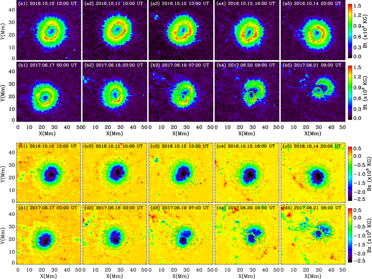
Figure 6. Transverse magnetic field maps of the stable sunspot (panels (a1)–(a5)) and the decaying sunspot (panels (b1)–(b5)), and vertical magnetic field maps of the stable sunspot (panels (c1)–(c5)) and the decaying sunspot (panels (d1)–(d5)). The contours indicate the inner and outer boundaries of the sunspot as seen in the continuum intensity.
Download figure:
Standard image High-resolution imageAnother difference between the stable and decaying sunspot is highlighted in the continuum intensity. For the decaying sunspot, the continuum intensity in the umbra is brighter. To obtain the variation of the continuum intensity in the decaying sunspot, the mean continuum intensities of the umbra and penumbra are calculated, respectively, and the results are shown in Figures 7(a1) and (a2). The blue symbols denote the decaying sunspot, and dark symbols denote the stable sunspot. From Figure 7(a1), it can be seen that the mean normalized intensity in the umbra of the stable sunspot remains at a value of about 0.32. However, the mean normalized intensity in the umbra of the decaying sunspot shows a clear trend of increase. For more information about the effect of stray light on mean continuum intensity, see the Appendix. This could be caused by the formation of the light bridge in the sunspot umbra during its decay. The appearance of the light bridge is the most striking manifestation of convection in the sunspot umbra (Borrero & Ichimoto 2011). And the intensity of the sunspot umbra increases with the formation of the light bridge (Louis et al. 2012). If so, this result suggests that more convective intrusions can be found in the umbra in the process of sunspot decay. Finding convective intrusions in the umbra of the decaying sunspot does not contradict simulations, as they suggest that the onset of the sunspot decay occurs in deeper layers (Panja et al. 2021; Strecker et al. 2021).

Figure 7. Left panels: variations of the mean continuum intensity, mean vertical magnetic field strength, and mean transverse magnetic field strength in the umbra of the stable and the decay sunspots during their evolutions. Right panels: same as the left panels, but only for mean values in the penumbra. The uncertainties are given by the standard deviation of these physical parameters for each observational time.
Download figure:
Standard image High-resolution imageIn the process of sunspot decay, although the umbra gradually brightens, the brightness of the penumbra was almost unchanged. For the penumbral region, the mean normalized intensity shows little change with a constant value of 0.78 for the decaying and the stable sunspots, as shown in Figure 7(a2).
The variations of mean vertical magnetic field strengths in the umbra and penumbra of the sunspots are shown in Figures 7(b1)and (b2). The mean vertical magnetic field strengths in the umbra and penumbra of the stable sunspot remain steady during the observational time. For the decaying sunspot, the mean vertical magnetic field strength gradually declines in the umbra but gradually rises in the penumbra. Figures 7(c1) and (c2) show the variations of mean transverse magnetic field strengths in the umbra and penumbra of the sunspots. For stable sunspots, the changes of the mean transverse magnetic field strengths in the umbra and penumbra are small. Although the penumbra of the sunspot first disappears in the process of sunspot decay, the change of umbra should not be ignored. For the decaying sunspot, the mean transverse magnetic field strengths in both the umbra and penumbra decrease, but the decrease of the umbra occurs at an earlier time.
3.2. Ic –B, Ic –γ, Ic –Bz , and Ic –Bz Relations at Solar Disk Center for 10 Selected Sunspots
To check whether the relations for the decaying sunspot contain more scattered pixels, especially in the relations of Ic –Bt and Ic − γ, we analyzed another four stable sunspots and four decaying sunspots. These sunspots are located around the disk center (μ > 0.95) at the selected observational time. Figure 8 shows their continuum intensity images, including two sunspots discussed in Section 3.1. The top panels of Figure 8 show the stable sunspots, which have a fully annular penumbra. The bottom five panels are the decaying sunspots that have lost part of their penumbra or have light bridges in their umbra. Some sunspot parameters are also given in Figure 8, including their location (μ), sunspot area (A), and the averaged umbral intensity (Iu).
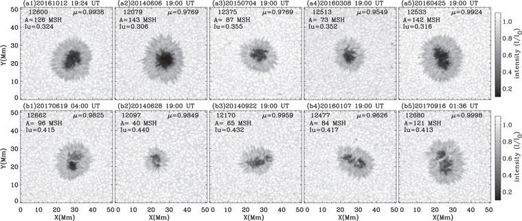
Figure 8. The continuum intensity images for the stable (top) and decaying sunspots (bottom) around the solar center.
Download figure:
Standard image High-resolution imageFrom Figure 8, it can be found that the umbral brightnesses of all decaying sunspots are higher than those of the stable sunspots. The umbral intensity of the largest decaying sunspot (sunspot of NOAA AR 12680, Iu = 0.413) is much brighter than that of the smallest stable sunspot (sunspot of NOAA AR 12513, Iu = 0.352). This reveals that the brightness of sunspots is associated with the sunspot evolution. Earlier observations show that the small sunspots are brighter than large sunspots (Martinez Pillet & Vazquez 1993; Mathew et al. 2007). We find that not only the sunspot size but also the evolution state of sunspots should be considered when studying sunspot brightness.
The Ic –B, Ic − γ, Ic –Bz , and Ic –Bt relations for the stable sunspots and decaying sunspots at the selected time are shown in Figure 9. The first row is for the stable sunspots, while the second row is for the decaying sunspots. Different colors in the scatter plots indicate different sunspots.
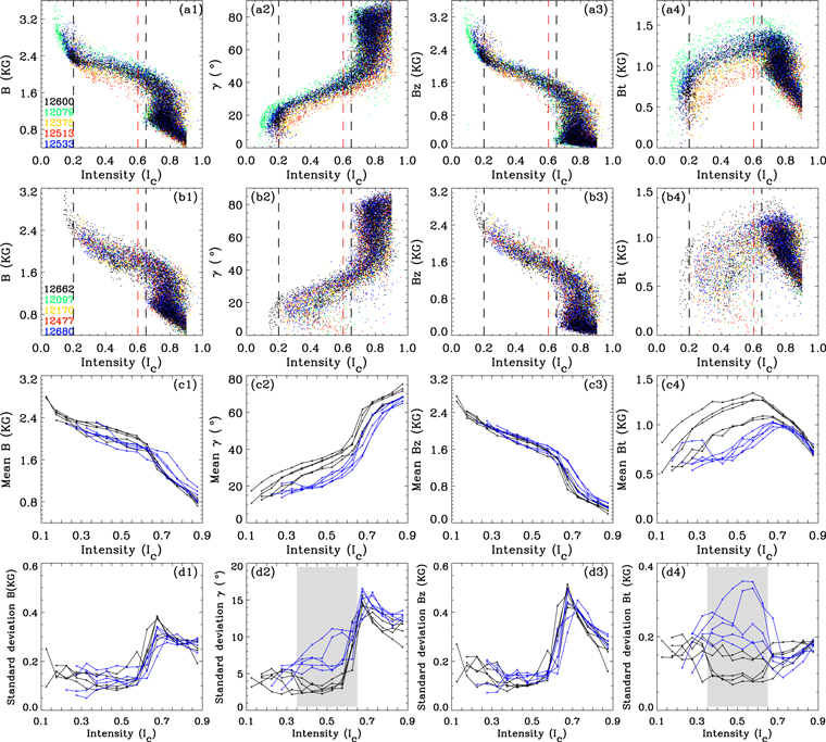
Figure 9. (a1–a4) Scatter plots of Ic –B, Ic − γ, Ic –Bz , and Ic –Bt relations in the stable sunspots. (b1–b4) Scatter plots of the relations in the decaying sunspots. (c1–c4) The mean values in each Ic = 0.05 interval for 10 sunspots. (d1–d4) The standard deviation of magnetic field values in each Ic = 0.05 interval for 10 sunspots. The black and blue lines are for the stable and decaying sunspots, respectively.
Download figure:
Standard image High-resolution imageThe profiles of the Ic –B, Ic − γ, Ic –Bz , and Ic –Bt relations are roughly the same for different stable sunspots. Among these five stable sunspots, the sunspot of NOAA AR 12079 is prominent (see the green points in Figures 9(a1)–(a4)). This sunspot has a stronger B and Bz and a higher value of Bt in the continuum intensity interval of Ic < 0.7. By tracking the evolution of this sunspot, we found that there is still a slow increase in the area of this sunspot after the chosen time. We speculate that the sunspot has just formed a relatively stable structure, although other mechanisms cannot be ruled out.
In general, large sunspots turn out to be darker and to have larger magnetic field strength (Mathew et al. 2007; Leonard & Choudhary 2008). However, this is not applicable to the decaying sunspots. For the five decaying sunspots, the sunspot of NOAA AR 12680 has the largest area, but it can be seen from Figure 9(b1) that its magnetic field strength is weaker than that of the sunspot of NOAA AR 12662. From the Ic –Bz relationship of the stable sunspots, it can be seen that Bz versus Ic show a significant linear correlation in the intensity interval of 0.25–0.65. In this interval, one continuum intensity value corresponds to only a small range of vertical magnetic field value. Thus, it is normal to find an invariance of the vertical magnetic field value on the boundary of the umbra and penumbra.
Comparing Figures 9(a1)–(a4) and (b1)–(b4), there are noticeable differences in the relationship for the stable and decaying sunspots. In the Ic –B relation, the sharp change of the B with the Ic in the umbra of the decaying sunspot is absent. In the Ic − γ relation of the decaying sunspot, there are more scattered points with small γ (<20°) in the intensity interval of 0.2–0.65. From the Ic –Bz of the decaying sunspot, it can be seen that the maximum of Bz decreases. And the Ic –Bt of the decaying sunspot is more scattered. The number of points with small Bz and high brightness increases.
The mean values in Ic = 0.05 intervals of the sunspots are shown in Figures 9(c1)–(c4). Figures 9(c1)–(c4) clearly show the difference between the stable and decaying sunspots in the Ic –B, Ic − γ, Ic –Bz , and Ic –Bt relations. The differences in the Ic − γ and Ic –Bt relations of the decaying sunspots can be seen from Figures 9(c2) and (c4). The Ic − γ relations of the decaying sunspots (blue curves) shift to the smaller γ values in each Ic interval. The differences of Ic –Bt between the decaying and stable sunspots mainly appear in the umbral regions. The Ic –Bt relations of the decaying sunspots shift to higher continuum intensity, and the mean values of each interval in the umbra are smaller.
Figures 9(d1)–(d4) show the standard deviations of magnetic field in each Ic = 0.05 interval of sunspots. By comparing decaying sunspots with stable sunspots, it can be found that the standard deviation values in the Ic − γ and Ic –Bt plots of decaying sunspots are larger in the umbra−penumbra transition (0.35 < Ic < 0.65; see the gray region of Figures 9(d2) and (d4)). In the Ic − γ relationship of decaying sunspots, the standard deviations are around two times higher in the interval of 0.35 < Ic < 0.65 compared with the stable sunspot.
4. Conclusion and Discussion
The relationships between continuum intensity and the magnetic field vector in the stable and decaying sunspots are investigated in this paper by using the deconvolved HMI data. For the stable sunspots, the results of Ic –B scatter plots are consistent with those of the earlier studies (Stanchfield et al. 1997; Mathew et al. 2004; Jaeggli et al. 2012; Tiwari et al. 2015; Sobotka & Rezaei 2017). In our results, we found a sharp variation of B at Ic < 0.2, a gradual change in B at 0.2 < Ic < 0.65, and a sharp decrease in B at Ic > 0.65; see Figure 3. Further, the Ic –Bz relationship is similar to the Ic –B relationship except that Bz does not decrease as rapidly as B with increasing Ic (in the region of Ic > 0.65; see Figure 4). This relationship is comparable with the results obtained by Mathew et al. (2004). Finally, the Ic –Bt relationship is nonlinear, which differs from the near-linear relationship found by Mathew et al. (2004). The difference in the Ic –Bt plot between our result and theirs may be due to the use of sunspots at different evolutionary stages. Other important influencing factors are the spatial resolution, optical quality contrast of the instruments, and different heights of sampled lines.
By comparing the relationship between the stable sunspots and decaying sunspots, we have found that the points are more scattered in the relationship of the decaying sunspots, especially in the plots of Ic − γ and Ic –Bt ; see Figure 9. The scattered region is mainly distributed in the umbra–penumbra transition (0.35 < Ic < 0.65). For example, in the Ic –Bt relationship of the decaying sunspot, the standard deviation increased 2.7 times in the interval of 0.6 < Ic < 0.65 over about 3 days. And this scatter is increased in the process of the sunspot decay. That is, the older the sunspot, the greater the scatter in the relationship plots. Moreover, the bifurcation in the plot of Ic –Bt is connected with the light bridge; see Figure 5. The formation of the light bridge causes the fragmentation of the sunspot, which means that the convection in the umbra is becoming more intense in the process of the sunspot decay. And the bifurcation in the plot of Ic –Bt may indicate that the umbral regions separated by the light bridge develop different geometries and temperatures as the sunspot decays.
In addition, we found that the continuum intensity of the umbra in the decaying sunspot is brighter; see Figure 7. The umbra of the decaying sunspot (NOAA 12662) is brighter than that of the stable sunspot (in NOAA AR 12600). The mean continuum intensity of the decaying umbra increases with time, but that of the stable sunspots remains constant. Note that the brightness of the penumbra changes little with a constant value of 0.78 during the decay of the sunspot. It is important to note that this is not a statistical result. But this result supports the statistical finding of Mathew et al. (2007), who found that the umbral mean brightness decreases substantially with increasing umbral size. As the sunspot decays, the umbral region becomes smaller in size and is accompanied by the enhanced continuum intensity. The umbral brightness increases during the decay, presumably due to convective intrusions from deeper layers. The light bridge is an example of convective intrusion, with the loss of stability of the umbral–penumbral boundary. Strecker et al. (2021) proposed that the onset of sunspot decay is not visible in the photosphere but occurs in deeper layers with the fluting instability. The increase of the mean continuum intensity of the umbra during sunspot decay is presumably due to convective intrusions from deeper layers, which would support the idea proposed by Strecker et al. (2021), that is, the sunspot decay originates in deeper layers. More research is needed.
It is important to investigate the factors that influence the brightness of sunspots for sunspot theory, since a reasonable answer must be found why the umbrae of larger sunspots are darker. One factor that probably plays a role is that the larger sunspots have stronger magnetic field strengths (Livingston 2002). Stronger magnetic fields can inhibit more energy transport by convection. Earlier observations suggested that the umbral intensity varies over the sunspot area (Kopp & Rabin 1992; Martinez Pillet & Vazquez 1993; Mathew et al. 2007) or the solar cycle (Watson et al. 2011; Rezaei et al. 2012; Norton et al. 2013). In our studies, we found that the continuum intensity of the umbra is associated with the evolutionary stage of the sunspot. To explain the brightness variation of the sunspots, Schüssler (1980) proposed that the brightness of the sunspots relates to the age of subphotospheric flux tubes, and Yoshimura (1983) suggested that it may be influenced by the depth of the flux bundles forming the sunspots. The increase of the umbral brightness in the decaying sunspot hints that the flux tube of the umbra changes in the process of the sunspot decay.
The change of the horizontal magnetic field in the penumbra is a significant process during the sunspot decay (Watanabe et al. 2014; Rempel 2015; Verma et al. 2018). According to the analysis of the sunspot in the AR 12662, it can be found that not only the horizontal magnetic field of the penumbra changes but also the magnetic field of the umbra changes during the decay of the sunspot. In the process of the sunspot decay, the strengths of the horizontal magnetic field in the umbra and penumbra decrease, but the strength of the horizontal magnetic field in the umbra decreases first (see Figure 7). These results suggest that the change of the umbra should not be ignored when studying the decay of the sunspot penumbra. The umbral and penumbral decay may be an interdependent and simultaneous process.
Although the differences in the relations between the continuum intensity and the magnetic field vector for the stable and decaying sunspots were analyzed, it is still not clear why the relations show considerable scatter in the decaying sunspots. The change of the relation for the decaying sunspots is relevant to the horizontal force balance in sunspots (Martinez Pillet & Vazquez 1993). The change of relations of the decaying sunspots may be related to the mechanism of sunspot decay. The decay of the sunspot is a process of losing balance. Either the gas pressure of the sunspot is changing faster than the magnetic pressure, or its magnetic pressure changes faster. In our cases, it is clear that the magnetic field strength decreases with time during the sunspot decay. This implies that the magnetic pressure is decreasing in the process of the sunspot decay. However, it is not easy to determine the change of the gas pressure in the sunspot. Mathew et al. (2004) found that the gas pressure is lower than the magnetic pressure in the umbra. In contrast, Jaeggli et al. (2012) suggested that the dissociation of H2 in the umbra atmosphere would rapidly increase the gas pressure, which would slow down the sunspot decay. The variation of the plasma β during the sunspot decay should be given more attention. In addition, our studies are restricted to regular sunspots. Magnetically complex sunspots may show different relations between the continuum intensity and the magnetic field vector. Ultimately, we wish to emphasize that it is important to study the decay process of different types of sunspots separately.
We thank the SDO/HMI teams for the data support. This work is partially supported by the National Key R&D program of China under grant No. 2018YFA0404204. This work is sponsored by the National Science Foundation of China (NSFC) under grant No. 11873087, by Yunnan Science Foundation for Distinguished Young Scholars under No. 202001AV070004, and by Yunnan Key Laboratory of Solar Physics and Space Science under No. 202205AG070009.
Appendix
Figure 10 shows the difference of the total magnetic field strength maps (panels (a1)–(a3)), transverse magnetic field maps (panels (b1)–(b3)), and magnetic inclination angle maps (panels (c1)–(c3)) before and after applying the scattered-light correction. As can be seen from Figures 10(a1)–(a3), the maximum total magnetic field values are stronger after applying the scattered-light correction. The values of the transverse magnetic field and magnetic inclination angle of the sunspot after calibration of stray light are not very different from their original values.
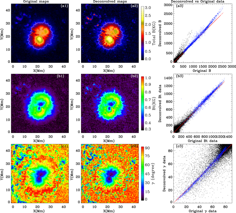
Figure 10. Difference of the total magnetic field strength maps (panels (a1)–(a3)), transverse magnetic field maps (panels (b1)–(b3)), and magnetic inclination angle maps (panels (c1)–(c3)) before and after applying the scattered-light correction. The third column shows the results of original data vs. the deconvolved data in the entire frames of the first column and second column. The white contours and blue circles are similar to those in Figure 1.
Download figure:
Standard image High-resolution imageAs can be seen from the plots in Figures 7(a1) and (a2) that the mean continuum intensity does not vary with time in both the umbra and penumbra of the stable sunspot. For the decaying sunspot, the mean continuum intensity in the umbra increases with time, but in the penumbra it remains constant. It is common for smaller umbral cores to look brighter. One expects that the smaller the area, the more severely they are affected by stray light. And the umbral core becomes smaller in size as the sunspot decays. Thus, the increase of the mean continuum intensity in umbra during the decay of the sunspot may be due to the larger contamination levels. However, this is only true as long as the brightnesses of all sunspots with different sizes are equal. Mathew et al. (2007) estimated the contamination levels of the sunspots with different brightness–size relationship by using the simulations and the Michelson Doppler Imager data. They found that when there is a negative correlation (smaller sunspots are brighter) between umbra intensity and sunspot size, the contamination levels of larger sunspots are always larger. This means that not all small sunspots get the most stray-light contamination. As the umbrae become smaller, the contamination levels may decrease. Thus, the increase in the umbra intensity of the decaying sunspot cannot be completely attributed to the increase of the stray-light contamination.
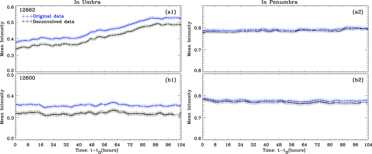
The results with stray-light-corrected data confirm this view. Figure 11 shows the evolutions of mean continuum intensity of the sunspots before (blue) and after (black) stray-light calibration with the PSF. The top row corresponds to the temporal evolution of the stable sunspot in NOAA AR 12662, and the bottom row is for the decaying sunspot in NOAA AR 12600. It can be seen from the figure that the variation trend of mean continuum intensity obtained from the data before and after is consistent. Thus, we conclude that the observed increased brightness for the decaying sunspot in Figure 7 reflects a real tendency of the decaying sunspot.
Figure 11. The evolution of mean continuum intensity in the umbra and penumbra of the stable sunspot (panels (a1) and (a2)) and the decaying sunspot (panels (b1) and (b2)). The blue lines show the mean continuum intensity computed with the original continuum intensity of HMI. The black lines correspond to the result of the deconvolved HMI maps.
Download figure:
Standard image High-resolution image