


Abstract
Magnetohydrodynamic waves are ubiquitously detected in the finely structured solar atmosphere. At the same time, our Sun is a highly dynamic plasma environment, giving rise to flows of various magnitudes, which can lead to the instability of waveguides. Recent studies have employed the method of introducing waveguide asymmetry to generalize "classical" symmetric descriptions of the fine structuring within the solar atmosphere, with some of them introducing steady flows as well. Building on these recent studies, here we investigate the magnetoacoustic waves guided by a magnetic slab within an asymmetric magnetic environment, in which the slab is under the effect of a steady flow. We provide an analytical investigation of how the phase speeds of the guided waves are changed, and where possible, determine the limiting flow speeds required for the onset of the Kelvin–Helmholtz instability. Furthermore, we complement the study with initial numerical results, which allows us to demonstrate the validity of our approximations and extend the investigation to a wider parameter regime. This configuration is part of a series of studies aimed to generalize, step-by-step, well-known symmetric waveguide models and understand the additional physics stemming from introducing further sources of asymmetry.
Export citation and abstract BibTeX RIS

Original content from this work may be used under the terms of the Creative Commons Attribution 4.0 licence. Any further distribution of this work must maintain attribution to the author(s) and the title of the work, journal citation and DOI.
1. Introduction
Understanding the behavior of magnetohydrodynamic (MHD) waves has a long-standing position as an important field within solar atmospheric research. This is due to the ubiquitous presence of magnetic fields in the highly dynamic and structured solar atmosphere, which can then act as a natural waveguide for propagating MHD waves. The motivation for studying MHD waves guided by various solar atmospheric structures is two-fold: they can play a significant role in solar atmospheric heating, and they may also be used for purposes of diagnosing the solar plasma. This latter goal is achieved through the techniques of solar magnetoseismology (SMS), which combine theoretical results on MHD wave propagation with observational data, and utilize the calculated and measured properties of MHD waves (e.g., frequency, amplitude, phase speed, and group speed) to provide insights into the magnetic waveguide environment (see the reviews by Nakariakov & Verwichte 2005; Andries et al. 2009; Ruderman & Erdélyi 2009; Morton et al. 2012). Using SMS methods, the more elusive parameters of the solar plasma, such as the coronal magnetic field strength, may be determined indirectly (Nakariakov & Ofman 2001; Erdélyi & Taroyan 2008). By building simple MHD waveguide models such as magnetic flux tubes or slabs, these diagnostic studies become possible in a wide range of solar atmospheric features, ranging from global structures, including solar plumes (DeForest & Gurman 1998), prominences (Arregui et al. 2012), coronal loops (Banerjee et al. 2007; de Moortel 2009), to mid- or small-scale fine structures, including the magnetic pores (Keys et al. 2018), spicules (Zaqarashvili & Erdélyi 2009; Tsiropoula et al. 2012), X-ray and EUV bright points (Golub et al. 1974).
One of the favored forms of these fundamental models is the Cartesian geometry, which is used to describe interfaces and slab-like configurations. In a series of seminal studies Edwin & Roberts explored and summarized the characteristics of magnetoacoustic waves guided by these geometries. Roberts (1981a) studied the propagation of magnetoacoustic surface waves at a single magnetic interface. Next, two interfaces were considered, constructing the model of a three-layer symmetric magnetic slab waveguide system with field-free outer layers (Roberts 1981b), and then with a magnetic external region (Edwin & Roberts 1982). Recent advances have focused on the consequences of incorporating an asymmetric environment into the slab model. Allcock & Erdélyi (2017, 2018) investigated the model of an isolated magnetic slab embedded between two field-free regions of different temperatures. Zsámberger et al. (2018) and Zsámberger & Erdélyi (2020) then examined the slab embedded in the asymmetric magnetic environment. A multilayered asymmetric waveguides system has recently been studied by Shukhobodskaia & Erdélyi (2018) in the nonmagnetic case and by Allcock et al. (2019) with magnetic fields reintroduced into the configuration.
Another avenue to improve Cartesian models worth exploring is the inclusion of bulk background plasma motions in the equilibrium configuration. This addition helps capture another essential aspect of the solar atmosphere, namely, the wide-spread presence of flows. For example, the concentration of the magnetic flux in the solar chromosphere is able to generate a multitude of small plasma jets called spicules (Beckers 1972; de Pontieu et al. 2007). A similar feature, the macrospicules are long plasma jets that are common in polar coronal holes (Pike & Mason 1998). Furthermore, X-ray and EUV jets are often discovered in coronal holes and were observed intensively at first with the YOHKOH telescope by Shibata et al. (1992). The presence of different flow profiles affects the wave propagation, and perturbations may result in various categories of instabilities. For instance, the Kelvin–Helmholtz instability (KHI) occurs as a consequence of the mass flows in prominences (see Berger et al. 2010; Ryutova et al. 2010), the parabolic flow pattern of coronal mass ejections (CME) in the solar corona (Foullon et al. 2011, 2013; Ofman & Thompson 2011), and the twisting–untwisting motion of magnetic flux tubes in solar surges (Zhelyazkov et al. 2015). Other types of instabilities include the resonant flow instability (Tirry et al. 1998; Taroyan & Erdélyi 2002) and shear flow instabilities (Taroyan & Ruderman 2011). Most recently, Zaqarashvili et al. (2021) found that the dynamic kink instability of triangular jets can cause a complete breakdown of the MHD flows, which could result in the disappearance of spicules in solar atmosphere.
It is noteworthy that in their study of magnetic Kelvin–Helmholtz instabilities, Foullon et al. (2011) proposed the three-layered system configuration consisting of the dense solar ejecta, the CME sheath, and the low-density corona. Möstl et al. (2013) interpreted the CME boundary as a magnetic slab sandwiched between asymmetric magnetic external layers. Barbulescu & Erdélyi (2018) analyzed the effects of a steady flow and the propagation of magnetoacoustic waves in a field-free asymmetric slab with a steady flow in the central region, and found that the external asymmetry can reduce both the KHI threshold and the cutoff speed of the waves guided by such a geometry. They proceeded to apply this model to the CME flank region and provided and estimate for the density of the CME ejecta, noting that the incorporation of asymmetric external fields into the model could further improve the results and explain the observed absence of the KHI between the CME core and flank regions.
Within this paper, we study the Kelvin–Helmholtz instability and investigate the behavior of propagating MHD waves in magnetic slab subject to a steady flow, which is embedded in an asymmetric magnetic environment. First, we derive a full dispersion relation for the propagation of waves along the slab by using the ideal MHD equations. In the next section, we consider the special case of weak asymmetry, which allows us to decouple the single dispersion relation into two equations: the equation containing the tanh term corresponds to the quasi-sausage mode and the one containing the coth term to the quasi-kink mode. We then obtain approximate solutions to the decoupled dispersion relation in the limits of a thin slab and zero-β plasma. Next, we use these results to determine an analytical limit for the flow speed at which the KHI first occurs. Finally, we present numerical results of the full dispersion relation and further compare them to approximate solutions in the Appendix.
2. Full Dispersion Relation
Let us consider a model of a three-dimensional asymmetric magnetic slab waveguide filled with ideal, inviscid plasma and permeated by an equilibrium magnetic field in the z-direction. The waveguide is divided into three layers by two plane interfaces placed at x = ± d. The equilibrium pressures, pj , densities, ρj , temperatures, Tj , and vertical magnetic fields, B j = (0, 0, Bj ) can be summarized as follows:
where j = 0 denotes quantities inside the slab, while j = 1 and j = 2 stand for parameters in the left- and right-hand-side environmental regions, respectively. In addition, the central region is subject to a steady flow V 0 = (0, 0, V0). An illustration of this equilibrium configuration is shown in Figure 1.
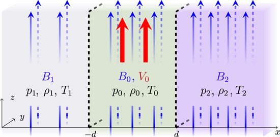
Figure 1. Equilibrium configuration for the magnetic slab (∣x∣ ≤ d) embedded in an asymmetric magnetic environment (x < −d and x > d). The blue arrows represent the magnetic fields in the  -direction. The red arrows illustrate the steady flow
  inside the magnetic slab.
Download figure:
Standard image High-resolution image2.1. Ideal Magnetohydrodynamic (MHD) Equations
We use the ideal MHD equations to model the behavior of the plasma and magnetic field interactions in the slab system, similarly to Zsámberger et al. (2018). These equations can be summarized as follows:
where μ is the magnetic permeability of free space, and γ is the ratio of specific heats, which are constant all throughout the configuration. We require that the condition of total pressure balance is met by the background parameters:

We linearize these equations by introducing a small perturbation to the equilibrium quantities such that
where j = 0, 1, 2, and the variables with primes denote the perturbations. These perturbations must remain linear, which we ensure by the condition  , where f denotes an equilibrium quantity and
  its perturbation. After performing some algebraic transformations, the system of linearized ideal MHD equations may be summarized as follows:

where  is the sound speed of a given region (j = 0, 1, 2).
2.2. Plane Wave Solutions
To proceed, we assume that disturbances are independent of the y-component, v = (vx , 0, vz ) and b = (bx , 0, bz ) and that the small perturbations can be written in the form of a Fourier series, allowing us to look for so-called plane wave solutions,

where the hat notation denotes the x-dependent amplitudes of the wave solutions for corresponding disturbances, k is the z-component of the vector wavenumber κ = (kx , ky , k) showing the propagation of MHD waves along the slab, and ω is the angular frequency.
After we substitute the plane wave solutions defined above into the linearized ideal MHD equations, they can be combined and reduced to a single ordinary differential equation for each of the three regions in the model:

where

and
Here,  is the Alfvén speed of a region, and
  is defined as the tube or cusp speed (for j = 0, 1, 2). Further, Ω = ω − kV0 is the Doppler-shifted frequency, which appears in the equations due to the presence of the background flow in the central region. Confirming our results so far, if we reduce the external magnetic fields to zero, Equation (5) becomes the same as Equation (4) in Barbulescu & Erdélyi (2018) for a magnetic slab in an asymmetric nonmagnetic environment.
In order for waves to be trapped by the slab, all perturbations must vanish at infinity by ensuring  , hence the exterior parameters mj
2 are supposed to be positive in Equation (5). Note that the interior parameter
, hence the exterior parameters mj
2 are supposed to be positive in Equation (5). Note that the interior parameter  may take both positive or negative values in Equation (5). We then obtain the general solution of Equation (5) in each region as the following linear combination of the hyperbolic functions:
where A, B, C, and D are arbitrary real constants.
2.3. Boundary Conditions
We need to apply two linearized boundary conditions across the two interfaces at ± d. First, the Lagrangian displacement has to remain continuous at x = ± d:
Further, the continuity of the total (plasma plus magnetic) pressure perturbation has to be kept across the interfaces:
where  (for j = 0, 1, 2).
2.4. Dispersion Relation
The four boundary conditions give us a homogeneous system of four linear equations with variables A, B, C, and D, which we can write more compactly in matrix form as Ax = 0
where  and
and  , for j = 0, 1, 2. Further, the Λ coefficients are defined as
The solutions of the coefficient matrix A will be nontrivial, if the determinant ∣ A ∣ = 0. Therefore,
In the end, using the original notation explicitly containing the characteristic speeds, we obtain the full dispersion relation for MHD waves in a magnetic slab subject to a background flow and embedded in an asymmetric magnetic environment as:
where  .
.
Note that we could recover the dispersion relation studied by Zsámberger et al. (2018), Zsámberger & Erdélyi (2020) directly by removing the steady flow, i.e., V0 = 0, hence, reducing Ω to ω. If instead the magnetic fields outside the slab  and
and  are removed, it is possible to recover Equation (11) derived by Barbulescu & Erdélyi (2018). If we remove both the steady flow and the external magnetic fields, the dispersion relation (Equation (20)) of Allcock & Erdélyi (2017) could be recovered, confirming that our results are consistent with recent asymmetric slab studies. It can be shown that the results also agree with the study performed by Nakariakov & Roberts (1995), if the only flow is in the central region of their symmetric model, and the magnetic and plasma parameters are made symmetric in ours.
In the following section, we will utilize a few approximations of the dispersion relation derived here, in order to find analytical solutions for its limiting cases.
3. Approximations
The full dispersion relation (Equation (11)) is a complicated transcendental equation so that we cannot determine the solutions analytically. Therefore, to understand the behavior of the MHD eigenmodes in this new slab system, in this section, we derive some analytical approximations of Equation (11) that are relevant in solar physics, such as the weak asymmetry, thin-slab, and zero-beta limits.
3.1. Weak Asysmmetry
It is apparent that the dispersion relation (Equation (11)) is a single equation for all eigenmodes of the slab in an asymmetric environment. However, dispersion relations governing symmetric slab systems are divided into two separate equations for the two main types of eigenmodes, with the tanh and coth terms corresponding to the sausage and kink modes (see, e.g., Edwin & Roberts 1982).
When the asymmetry is weak, the densities, pressures and magnetic fields on the left side of the slab are the same order as on the right side, i.e., Λ1 ≈ Λ2, and the dispersion relation (Equation (11)) can be factorized as
Using the original notation yields the weakly asymmetric dispersion relation in the following form:
Similarly to dispersion relations of symmetric slab configurations, Equation (12) consists of two independent equations, with one of them describing the so-called quasi-sausage modes (tanh version), and the other one governing the quasi-kink (coth version). This is analogous to the dispersion relation (20) in Zsámberger et al. (2018), where the properties of these mixed eigenmodes are also described in some further detail.
Moreover, if the environment is made entirely symmetric (so that p1 = p2 = pe , ρ1 = ρ2 = ρe , B1 = B2 = Be ), Equation (12) reduces to the "classical" dispersion relation for waves propagating along a magnetic slab embedded in a symmetric magnetic environment derived by Edwin & Roberts (1982), which has the following form:
3.2. Thin-slab Approximation
Supposing the propagation of waves happens in a slender slab, the wavelength of the waves is much longer than the width of the slab, i.e., kd ≪ 1. This approximation has applications to various solar phenomena, such as prominences (Arregui et al. 2012), magnetic bright points (Liu et al. 2018), sunspot light bridges (Yuan et al. 2014), and sunspot light walls (Yang et al. 2016, 2017).
Recall that the interior parameter  of Equation (5) could be either positive or negative. Therefore, the quasi-sausage and quasi-kink eigenmodes can be further grouped by two wave modes
  and
and  , which we shall call surface and body wave modes, respectively. Surface waves have their maximum amplitude at the slab boundaries and are evanescent within the slab, whereas the amplitude of body waves remains spatially oscillatory in the central slab region as well (see Roberts 1981a; Allcock & Erdélyi 2018).
In the following subsections, we will study surface and body mode solutions to the approximate dispersion relation in further detail.
3.2.1. Surface Waves 

First, let us consider the quasi-sausage surface modes, substituting  into Equation (12) for
  . In this limit, m0
d ≪ 1; this implies that
. In this limit, m0
d ≪ 1; this implies that  , and the dispersion relation (Equation (12)) becomes
For the slow mode, we obtain the solution with  as kd → 0, in which case Equation (13) yields
where
This mode can exist as a stable oscillation when either cT1 > cT0 + V0 and cT2 > cT0 + V0, or c1 < cT0 + V0 < vA1 and c2 < cT0 + V0 < vA2, while in other cases, Rv
might be negative or complex, and instabilities might occur. Depending on which set of conditions is met, the slow quasi-sausage surface mode approaches  either from above or below as we consider ever thinner slabs (kd → 0).
Although Barbulescu & Erdélyi (2018) did not employ the weak asymmetry approximation in his study of an internal flow in a slab placed in an asymmetric nonmagnetic environment, these results are still comparable to his Equation (13). In both cases, the Doppler-shifted phase speeds of the slow quasi-sausage surface mode tend to the internal tube speed, and a further flow-dependence is present in the terms proportional to the dimensionless slab width. In our case, however, this term also contains a complex dependence on the external magnetic fields through the external Alfvén and tube speeds, resulting in a change in the exact behavior of the phase speeds as kd → 0.
For the fast mode, the trapped thin-slab solution only exists when the external sound speeds are the same, i.e., c1 ≈ c2 ≈ ce
. In this case, we substitute  into the dispersion relation and find the solution as

where
for min (vA1, vA2) > ce . This is a solution that approaches the common external sound speed from above as we consider ever thinner slabs or longer wavelengths (kd → 0). If the sound speeds become weakly asymmetric, the fast quasi-sausage surface mode solution will have a cutoff at the lower external sound speed value, beyond which the solution becomes leaky (which we do not investigate in the current paper). This result is comparable to Equation (16) of Roberts (1981b), in case the flow is removed and the environment of the slab is made symmetric. Unfortunately, a direct comparison to Barbulescu & Erdélyi (2018) is not possible, as in the lack of external magnetic fields, their investigation would have simply reduced to the symmetric case for the fast quasi-sausage modes while strictly excluding leaky domains.
Next, we consider the quasi-kink surface mode, substituting  into Equation (12). In the thin-slab limit,
  , and the dispersion relation in Equation (12) becomes
Similarly to the case of the fast quasi-sausage modes, when the external Alfvén or tube speeds are asymmetric, cutoff frequencies and the possibility of leaky modes are introduced, which we do not examine in further detail in this paper. For some examples of this behavior (see, e.g., Zsámberger et al. 2018; Zsámberger & Erdélyi 2020). Avoiding leaky modes, we can only proceed further with our approximation in the case when the external Alfvén speeds are the same, i.e., vA1 ≈ vA2 ≈ vAe
. Then, following the derivation shown in Edwin & Roberts (1982), when vAe
/vA0 is not of the order of kx0, we find the solution by substituting  , and it takes the following form:
where
This solution approaches the external Alfvén speed from below when  , and therefore max (c1, c2) < vAe
, and the coefficient Rv
is a positive real number. In the symmetric and static case, this mode corresponds to the one described in Equation (18) of Edwin & Roberts (1982).
, and therefore max (c1, c2) < vAe
, and the coefficient Rv
is a positive real number. In the symmetric and static case, this mode corresponds to the one described in Equation (18) of Edwin & Roberts (1982).
A further kink mode solution can be found with symmetric external tube speeds (cT1 = cT2 = cTe
). The phase speed of this solution tends to  as kd → 0:
If the flow is removed from the system, this solution corresponds to Equation (18) of Edwin & Roberts (1982).
Alternatively, when vAe ≪ vA0, a different kind of solution can be obtained in the thin-slab limit. In order to exclude all leaky domains, we suppose that the external Alfvén speeds are the same, in which case this solution can be described as
In the fully symmetric case with no background flows present, this reduces to Equation (19) of Edwin & Roberts (1982), describing a kink mode that approaches the external Alfvén speed from above.
3.2.2. Body Waves

If we take  in the decoupled dispersion relation (Equation (12)), it can be transformed into an equation that contains only trigonometric functions rather than hyperbolic ones. For this case of the body waves, we define
  The dispersion relation (Equation (12)) can then be rewritten as:
In order to identify all possible body modes, we look for solutions where the last term of the dispersion relation remains finite (see, e.g., Roberts 1981b). For slow body modes, we must have  , and find the solution in the form of
  for some η > 0 that is to be determined. In the case of the quasi-sausage mode, for
  to be bounded, q0
d needs to converge to the roots of
to be bounded, q0
d needs to converge to the roots of  , i.e., q0
d = n
π for
, i.e., q0
d = n
π for  . Thus,
Rearranging this equation yields η = ηn for n = 1, 2, 3 ⋯ as
Manipulating the dispersion relation in a similar manner for the quasi-kink mode, we arrive at  for
for  . Therefore,
Therefore, the behavior of the Doppler-shifted quasi-sausage and quasi-kink body modes in a thin slab is given by
3.3. Zero-β Approximation
In the zero-β approximation, the plasma is cold in all three layers, i.e.,  , for j = 0, 1, 2. It follows that the sound speeds are negligible compared to the Alfvén speeds, i.e., c1/vA1 ≈ c0/vA0 ≈ c2/vA2 ≈ 0. This provides a good approximation of the solar coronal environment. We now have
for j = 1,2. The slow body waves are no longer present here, leaving only the fast body waves, which is analogous to the symmetric case studied by Edwin & Roberts (1982). So Equation (20) reduces to
Due to the condition of total pressure balance ( ) we could write the density ratios in terms of the characteristic speeds for any two regions i = 0, 1, 2 and j = 0, 1, 2 as

Substituting Equation (22) into the dispersion relation (Equation (20)), we obtain
For simplicity we can express this as
We are only interested in solutions that fall within the frequency range  and expect to determine ν in
 ![${{\rm{\Omega }}}^{2}={k}^{2}{v}_{{Am}}^{2}\,\tfrac{{\rho }_{m}}{{\rho }_{0}}\,\left[1+\tfrac{\nu }{{k}^{2}{d}^{2}}\right],$](https://content.cld.iop.org/journals/0004-637X/935/1/41/revision1/apjac7ebfieqn44.gif) where
where  Hence the quasi-sausage and quasi-kink modes solutions of the fast body waves are
These equations have an explicit dependence on the internal slab parameters, but they also possess a further implicit dependence on the external parameters of the slab system through the pressure balance condition expressed in Equation (22).
4. Instability
When there is a discontinuity in the velocity at the interface between two parallel hydrodynamic (magnetic field-free) layers, the fluids become unstable and generate vortices that can be modeled as vortex sheets. This instability is called a Kelvin–Helmholtz instability (KHI), and it occurs frequently in nature, for example, as the classic wind-over-water instability (Miles 1957). It also can be observed in solar corona (Foullon et al. 2011), in the interaction of the solar wind with the Earth's magnetosphere (Miura 1984; Hasegawa et al. 2004), and more recently in some astrophysical plasma jets (Kuridze et al. 2016; Zhelyazkov et al. 2018). Chandrasekhar (1961) analyzed two linear KHI cases in MHD, for a magnetic field parallel and perpendicular to the flow. The presence of a magnetic field produces a restoring force that can stabilize the KHI in the parallel case, while in the perpendicular case, there is no restoring force so the magnetic field has no effect on the flow.
We have established that the plane wave solutions of small perturbations are

All of these small perturbations are proportional to  ; therefore, the imaginary part of the angular frequency,
  , determines whether the system is stable or not.
- 1.If, the small perturbations would decay exponentially (stable modes).
- 2.If, the small perturbations would grow exponentially (unstable modes).


Hence for the instability, we require  .
.
4.1. Quasi-sausage Surface Modes in a Thin Slab
From Equation (14) for the slow quasi-sausage surface mode in the thin-slab approximation, we can express the angular frequency of this type of solution and analyze whether it is a real or a complex frequency in order to study instabilities. The system is unstable if  ; therefore we require
As the expression for Rv
contains all the external characteristic speeds, it encompasses several possible combinations of them, some of which yield a real, positive or negative value for Rv
, while others would make it imaginary. Furthermore, Rv
also contains the flow speed, V0, in several terms. Because of this, in order to express the critical flow speed beyond which the Kelvin–Helmholtz instability appears in the system, a cubic inequality in  would have to be solved for several different cases depending on the ordering of characteristic speeds, which we have opted not to include in this exploratory study of the asymmetric magnetic slab model under the effect of an internal background flow.
For the fast quasi-sausage surface mode in the thin-slab approximation, Equation (15) and the Rv coefficient it contains can be rearranged to yield
where
where  , ensuring that Rv
2 is positive and Rv
itself is a positive real number. For the instability, we require
, ensuring that Rv
2 is positive and Rv
itself is a positive real number. For the instability, we require  , and therefore
Next, we study the case when both  and
and  are true. Then the inequality can be rearranged to give

where
If we now suppose that A − 1 > 0, this provides us with a condition for the slab widths for which the results can be valid, namely,  . For the case when ce
−V0 < 0, the threshold for the onset of instability can be found as
. For the case when ce
−V0 < 0, the threshold for the onset of instability can be found as

When the flow speed is lower than this critical value, the magnetic fields present will be sufficiently strong to suppress the instability.
4.2. Quasi-kink Surface Mode in a Thin Slab
Next, we inspect the instability threshold for the quasi-kink surface modes in a thin slab described by Equation (17), when vA0 ≪ vAe . We require
where  to ensure that
  . In the case when
  and vAe
> V0, the threshold for instability becomes
and vAe
> V0, the threshold for instability becomes

For the kink mode that tends to the average external tube speed, the angular frequency can be expressed from the previous section as
For the instability, we require ω2 < 0, and therefore
When the conditions  and cTe
< V0 are met, this leads to the following expression for the instability limit:
and cTe
< V0 are met, this leads to the following expression for the instability limit:

On the other hand, when vAe ≪ vA0, the quasi-kink wave frequency is given as
which becomes unstable when ω2 < 0; therefore
In this case, the critical speed for the instability limit can be found as
Due to the wide variety of options available for choosing the characteristic speeds in each region, beyond the ones described in this section, several other interesting cases can be found when investigating the speed threshold for the onset of the Kelvin–Helmholtz instability. Similarly to the case described by Barbulescu & Erdélyi (2018), within the same asymmetric slab system, characterized by the same sound and Alfvén speeds, different modes can become unstable for different values of the background flow. This also means that the instability limits of different modes have to be investigated at the same time when analyzing the stability of a given slab system. Although in some cases at higher speeds multiple modes can be unstable at the same background flow speed value, the lowest KHI threshold speed has to be identified, as this is the one that marks the boundary between stable and KHI-unstable slab parameters.
In the following section, we illustrate this phenomenon using numerical solutions to the full dispersion relation, and we describe the effects of increased background asymmetry on the phase speeds and stability of eigenmodes.
5. Numerical Results
In order to complement our analytical findings and explore solutions within a wider parameter regime than what the abovementioned analytical restrictions allow for, in this section, we present numerical solutions to the full dispersion relation and instability limits determined from these results. In order to find the complex roots of the dispersion relation, we developed a module built on the Newton–Rhapson method utilizing the scipy package available in Python. A grid structure was set up on the solution space under investigation, and root finding was performed in every cell to ensure the identification of every local solution with a 1e−30 allowed error level. The module used for this work is a further developed version of the module utilized in our earlier work (Barbulescu & Erdélyi2018).
In order to obtain our results, we nondimensionalized the quantities appearing in the dispersion relation with respect to the Alfvén speed and introduced the Alfvén Mach number, MA0 = V0/vA0, to characterize the relative strength of the flow present in the central region of the slab. We prepared our figures with the choice of vA0 = 1; therefore in the following section, we did not specifically include new notation in the figures to indicate nondimensional speeds (as quantitatively, they will have the same value as their dimensional forms).
To obtain the solutions presented in this section, we used a root-finding method to solve the full dispersion relation in Equation (11). Figure 2 shows how the phase speeds of the solutions depend on the changing Alfvén Mach number for a fixed value of the slab width (corresponding to a thin slab, kd = 0.1). We have also indicated the characteristic speeds in the external regions and their Doppler-shifted values for the central slab region. The real part of the phase speeds is plotted in blue, while the two branches of the imaginary part (symmetric to the ω/kvA0 = 0 line) are shown in red in each of our figures.

Figure 2. Solutions of the full dispersion relation (Equation (11)) in (a) a symmetric slab of fixed width (kd = 0.1) and in (b) a weakly asymmetric slab of the same width. The real (imaginary) parts of the solutions are shown in blue (red). The characteristic speeds and density ratios used to prepare panel (a) were: c0 = 0.8vA0, c1 = c2 = 1.51vA0, vA1 = vA2 = 0.9vA0, and ρ1/ρ0 = ρ2/ρ0 = 0.5, while we used the weakly asymmetric parameters c0 = 0.8vA0, c1 = 1.51vA0, c2 = 1.33vA0, vA1 = 0.9vA0, vA2 = 0.9vA0, ρ1/ρ0 = 0.5, and ρ2/ρ0 = 0.6 for panel (b). In both figures, the inlet shows an enlarged view of the region in the black rectangle, where an additional small unstable region is present.
Download figure:
Standard image High-resolution imageThe panels of Figure 2 show that different types of solutions can exist in this particular slab system. Here, and in the following, we focus on the trapped solutions, for which both of the conditions  and
and  are fulfilled, and we will not discuss instabilities tied to modes with phase speeds in the leaky domains (
 or
or  , corresponding to cT1 < vph< vA1, cT2 < vph < vA2, c1 < vph, and c2 < vph, as well as the similar corresponding regions for negative phase speed values, indicated by gray hatching in all of our figures). In order to better highlight the effects of asymmetry, in Figure 2(a), we first present solutions obtained for a symmetric slab by using the following values of the characteristic speeds and density ratios: c0 = 0.8vA0, c1 = c2 = 1.51vA0, vA1 = vA2 = 0.9vA0, and ρ1/ρ0 = ρ2/ρ0 = 0.5. Then, Figure 2(b) shows how these solutions change when we introduce weak asymmetry by setting the background parameters to c0 = 0.8vA0, c1 = 1.51vA0, c2 = 1.33vA0, vA1 = 0.9vA0, vA2 =0.9vA0, ρ1/ρ0 = 0.5, and ρ2/ρ0 = 0.6.
It is easy to see from either panel of Figure 2 that the slow quasi-kink modes, whose phase speeds tend to the external tube speeds in the thin-slab limit, will be affected strongly by the flow. In the region between −cT2 and cT2, up to quite high values of the Alfvén Mach number, these waves are stable; however, at around MA0 = 2.5, the Kelvin–Helmholtz instability sets in for these modes (see the parabola-shaped red curve on the right). Once the phase speeds of the forward- and backward-propagating modes meet this way, for this specific configuration, the system remains unstable for all flow speeds width values greater than this threshold in both the symmetric and the weakly asymmetric cases.
In Figure 2(a), another unstable region can be seen as well, starting at around MA0 = 2. This, however, is tied to sausage modes whose phase speeds are close to the external sound speed (ce = c1 = c2 for the symmetric case). As we only focus on trapped oscillations in this study, these sausage modes have a cutoff at the external sound speed shortly after we reach high enough flow speeds to subject them to the KHI, as we have removed any solutions falling within the leaky regimes from the figures. This particular instability is unique to the symmetric case, because in the asymmetric system, the external sound speeds differ, lowering the cutoff frequency for the quasi-sausage modes and pushing the instability into the leaky domain (solutions not displayed in panel (b) of Figure 2). This example illustrates one of the several new cutoff frequencies that can be introduced due to the presence of asymmetry. For further examples of the new cutoff frequencies of trapped eigenmodes in a static magnetic slab enclosed in an asymmetric magnetic environment, see e.g. Zsámberger & Erdélyi (2020).
Using a high-resolution grid to obtain numerical solutions also reveals a third possible flow speed regime that can result in the onset of the Kelvin–Helmholtz instability at around MA =1.5. This unstable regime is present in both the symmetric and the weakly asymmetric cases, the details of which are shown in the inlets of the two panels in Figure 2. Although further examination shows that this instability is tied to a very small regime of both Alfvén Mach numbers and dimensionless slab widths, it still represents an important result, as it shows that in spite of the presence of external magnetic fields, the instability can still be triggered at much lower flow speeds than the thresholds marked by the previous two unstable regimes that we discussed.
Next, in Figure 3, we demonstrate the effect that the increase in density asymmetry can have on the solutions, even when the external Alfvén speeds are kept the same. To obtain these solutions, we used similar parameters to the previous figure for the sake of easy comparison: c0 = 0.8vA0, c1 = 2.59vA0, c2 = 1.33vA0, vA1 = 0.9vA0, vA2 = 0.9vA0, ρ1/ρ0 = 0.2, and ρ2/ρ0 = 0.6. This example illustrates the case of strong asymmetry, with the density on one side of the slab being 3 times as high as on the other side. This figure also serves as an extension to the analytical parts of our study, as the approximations obtained for the phase speeds of each eigenmode were derived for the case of weak asymmetry only, whereas using the full dispersion relation and finding numerical solutions to it allows us to explore the case of much stronger background asymmetry as well. To illustrate the close correspondence (specifically for the case of weak asymmetry) between the full solutions and some approximations of the full dispersion relation, we have included additional figures in the Appendix. Panel (a) of Figure 3 shows how the phase speeds of the solutions depend on the changing dimensionless slab width, kd, for a fixed value of MA0 = 2.1, while panel (b) displays the dependence of the phase speeds on the Alfvén Mach number for a fixed value of the slab width (corresponding to a thin slab with kd = 0.1). In both panels, we have indicated the characteristic speeds in the external regions and their Doppler-shifted values for the central slab region. As before, the real part of the phase speeds is plotted in blue, while the imaginary part is shown in red in each of our figures.
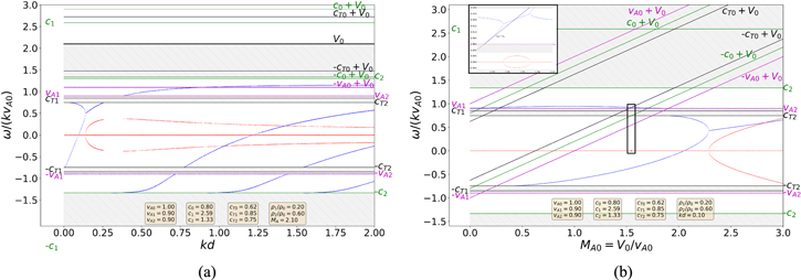
Figure 3. Solutions of the full dispersion relation (Equation (11)) in a strongly asymmetric slab system. Panel (a) shows the dependence of the phase speeds and the instability limit on the slab width with a fixed value of MA0 = 2.1, while panel (b) illustrates the same for a changing Alfvén Mach number with a fixed slab with of (kd = 0.1). The real (imaginary) parts of the solutions are shown in blue (red). The characteristic speed and density values used to obtain the solutions in both panels are: c0 = 0.8vA0, c1 = 2.59vA0, c2 = 1.33vA0, vA1 = 0.9vA0, vA2 = 0.9vA0, ρ1/ρ0 = 0.2, and ρ2/ρ0 = 0.6. The inlet in panel (b) shows a zoomed in view of the area in the bold black rectangle, where, similarly to the weakly asymmetric case shown in Figure 2, an additional instability region is present in a narrow range of Alfvén Mach numbers.
Download figure:
Standard image High-resolution imageWe can observe the same type of instabilities that we described in Figure 2 in panel (b) of Figure 3 too. Having located where the new KHI threshold is in this figure, we prepared a different diagram for Figure 3(a), which allows us to determine whether the modes will be stable or not for one fixed flow speed above the KHI threshold for the kd = 0.1 case, when the slab width is allowed to take different values. It is easy to see from this figure that the slow quasi-kink modes causing the instability in question are stable for very thin slabs. However, at somewhat larger, but still relatively small, values of the slab width, the phase speeds of the forward- and backward-propagating modes meet, and the system becomes unstable for all slab widths greater than this threshold value of approximately kd = 0.2. Similarly to the case of weak asymmetry, two further instability regimes could also be found in the strongly asymmetric slab system. One of these, the one attached to the lowest flow speeds, is displayed in the inlet of Figure 3(b). The other additional unstable region would be attached to the leaky quasi-sausage modes discussed above and have been removed from the figure. An additional group of solutions that appears only for larger slab widths and large negative to small positive values of the phase speed in Figure 3(a) is that of the harmonics of body modes, with no additional instabilities resulting from their presence for the chosen set of background parameters.
In Figure 3(a), other effects of the increased asymmetry can be observed beyond the somewhat changed phase speeds of the solutions too. First, due to the larger difference in background densities compared to Figure 2(b), in Figure 3(b), the sound speeds of the two environmental regions are more strongly separated too. This results in a wider range of phase speeds having to be excluded as leaky modes. Furthermore, the instability resulting from the shifting of the quasi-kink mode phase speeds now sets in at lower values of the Alfvén Mach number than in the weakly asymmetric case. This highlights an interesting consequence of the magnetic asymmetry implicitly present in the system (as the different density ratios require magnetic fields of different strength to be present in the external regions in order to maintain the shared value of the external Alfvén speed, vAe = vA1 = vA2). Although the KHI threshold is still relatively high in this slab system due to the restoring force of the strong external magnetic fields, the greater the asymmetry between the external regions is, the less effective this suppression of the instability seems to become.
6. Conclusions
The present study set out to further generalize the model family of asymmetric magnetic slabs (see, e.g., Allcock & Erdélyi 2018; Barbulescu & Erdélyi 2018; Zsámberger et al. 2018) with a focus on the concurring effects of destabilizing internal flows and potentially stabilizing asymmetric external magnetic fields. Namely, we carried out an analytical and numerical investigation of the effects of a steady flow on the propagation and instabilities of MHD waves in a magnetic slab embedded in an asymmetric magnetic environment.
We first obtained the full dispersion relation, which, unlike in the case of symmetric slabs, does not decouple into two separate equations for the general case. Next, we employed the approximation of weak asymmetry between the external regions of the model in order to derive an analytically more easily tractable decoupled dispersion relation, providing a separate description for the quasi-sausage and quasi-kink modes. In order to make further analytical progress, we focused on slabs that are thin compared to the typical wavelength of perturbations and provided some simple expressions for the angular frequencies of the surface and body eigenmodes in this system. To conclude the section, we provided a simplification of this general case specifically for the zero-β approximation. These equations defining the angular frequencies of asymmetric eigenmodes in terms of the characteristic speeds and densities present in the system were then also utilized to define the flow speed threshold, beyond which the shearing motions lead to the onset of the Kelvin–Helmholtz instability. Depending on the choice of parameters, especially the relative magnitudes of the internal flow and the magnetic fields in every region, as well as the degree of asymmetry between these magnetic fields, the instabilities might be suppressed by the stabilizing force arising from the inclusion of strong external magnetic fields, but this will not generally be true in every case. A further, detailed parametric examination of the model would be necessary to explore this possible suppression of instabilities.
Instabilities caused by flows play a critical role in the dynamics of the solar atmosphere and have a consequence in energy dissipation in the corona to heat the solar plasma. There are various possibilities to model solar structures affected by background flows and, for example, the critical flow speed for the KHI onset. In the future, a further useful tool to examine the eigenfunctions of such systems and carry out parametric studies can be the Large Eigensystem Generator for One-dimensional pLASmas, or LEGOLAS code (Claes et al. 2021). In the current paper, we are only concerned with magnetoacoustic waves propagating along the slab, parallel to the background magnetic fields; therefore we fixed ky = 0 and vy = 0. This means that the study of y-dependent Alfvén waves and the coupling between them and magnetoacoustic waves are beyond the scope of the current investigation. It must be acknowledged that choosing ky = 0 and a piecewise uniform configuration precludes us from exploring some further physical effects that influence the stability of the slab system. For example, Andries et al. (2000) studied coronal plumes and their environment by including a nonuniform transitional layer in a slab and a flux tube model while also allowing for the ky ≠ 0 case. They found that the resonant flow instability can occur at a lower velocity threshold than the KHI, which is a phenomenon that the current model cannot reproduce due to the chosen restrictions and focus. Beyond the resonant flow instability (Tirry et al. 1998), further mechanisms that could be studied in nonuniform cases and are very important in the field of solar atmospheric heating are, for example, resonant absorption (Goossens et al. 2011) and phase mixing (Ruderman & Erdélyi 2009).
While it is apparent that our study must accept certain limitations in order to focus on the effects of asymmetry, the asymmetric magnetic slab system under the effect of a steady central flow already provides several free parameters and a very rich problem to study both analytically and numerically. Furthermore, we can use the equilibrium configuration described in the current paper to model various asymmetric solar astrophysical waveguides. For example, it has been shown before that the asymmetric magnetic slab model provides a good approximation of CME flank regions and that the inclusion of external magnetic asymmetry may bring additional accuracy into their analysis (Foullon et al. 2011; Barbulescu & Erdélyi 2018). We can find further possible solar applications in the form of coronal hole boundaries (Banerjee 2012), prominences (Arregui et al. 2012), magnetic bright points of photosphere (Liu et al. 2018; Zsámberger et al. 2018), sunspot light bridges (Yuan et al. 2014), and sunspot light walls (Yang et al. 2016, 2017). Some of these have been modeled as static asymmetric slabs before (see, e.g., Zsámberger & Erdélyi 2020), but an extension of these models to incorporate flows captures more of the essential nature of these solar features and introduces additional physical phenomena to be studied.
One of the main motivation behind such a step-by-step generalization of asymmetric slab models is to provide the analytical basis and tools to carry out solar magnetoseismologic investigations and thus diagnose properties of solar plasma that might not be possible to measure directly. In the coming years, with the advent of the next generation of observational instrumentation, such as the Daniel K. Inouye Solar Telescope (DKIST) and the European Solar Telescope (EST), we will have an unprecedented temporal and spatial resolution available to apply these models and contribute to a better understanding of several magnetized structures within the Sun's atmosphere.
The authors are grateful to the UGRI scheme at The University of Sheffield for making the initiation of this research possible. N.Z. is grateful for the support of the University of Debrecen and the University of Sheffield. R.E. is also grateful to the Science and Technology Facilities Council (STFC, grant No. ST/M000826/1) for the support received. The authors also thank M. Barbulescu for making available the root-finding algorithm (at https://github.com/BarbulescuMihai/PyTES) that the code used during the numerical investigation was originally based on.
Appendix: Comparison of Solutions to the Full and Decoupled Dispersion Relations
In Sections 2 and 3, we derived the full dispersion relation for magnetoacoustic waves propagating along a magnetic slab placed in an asymmetric magnetic environment, where the slab is also subject to a bulk background flow. Then we proceeded to analytically describe the quasi-sausage and quasi-kink eigenmodes of this slab for the weak asymmetry and thin-slab approximations. In this Appendix, we show a close correspondence between the exact and approximate solutions by providing a set of figures containing numerical solutions to the equations providing the key points of this derivation, as we gradually employ first the weak asymmetry and then the thin-slab assumptions.
Equation (11), the full dispersion relation, provides an accurate description for magnetoacoustic waves propagating along a magnetic slab place in an asymmetric magnetic environment and under the effect of a steady background flow (under the assumptions of ideal MHD and linear perturbations to the system). It is, however, a transcendental equation that is, to the best of our knowledge, not possible to solve analytically for the general case. Therefore, to understand the behavior of eigenmodes and how they are influenced by the asymmetry and the flow present in the system, we had to analyze various limiting cases. In this Appendix, we compare the full solutions to the ones obtained after employing various approximations, with the aid of a series of figures depicting the phase speeds of eigenmodes in similar slab systems.
First of all, Figure 2(b) in Section 5 displays the solutions to the general dispersion relation (Equation (11)) using a fixed dimensionless slab width value of kd = 0.1 as well as the following characteristic speeds and density ratios: c0 = 0.8vA0,c1 = 1.51vA0, c2 = 1.33vA0, vA1 = 0.9vA0, vA2 = 0.9vA0, ρ1/ρ0 =0.5, and ρ2/ρ0 = 0.6. In Section 5, we discussed the possible sources of instability in this slab system, one of which would have belonged to leaky quasi-sausage modes and was excluded from the current study.
In the panels of our Figure 4 of this Appendix, prepared with the same characteristic speeds and density ratios as the full solution in Figure 2(b), we demonstrate that the behavior of the eigenmodes is qualitatively the same and quantitatively similar if we use certain approximations to obtain our solutions.

Figure 4. Solutions of the approximations of the dispersion relation. The real (imaginary) parts of the solutions are displayed in blue (red) in every case. Panel (a) shows quasi-sausage modes described by Equation (12), while panel (b) shows quasi-kink modes obtained from the same equation. Panel (c) displays the quasi-sausage mode solution obtained from Equation (13), and panel (d) provides quasi-kink mode solutions described by Equation (16). All solutions here were obtained using the same characteristic speeds and density ratios that we used in Figure 2(a), namely: c0 = 0.8vA0, c1 = 1.51vA0, c2 = 1.33vA0, vA1 = 0.9vA0, vA2 = 0.9vA0, ρ1/ρ0 = 0.5, and ρ2/ρ0 = 0.6.
Download figure:
Standard image High-resolution image
The first major analytical leap we took was introducing the approximation of weak asymmetry. This led us to the decoupled dispersion relation (Equation (12)). The first fundamental comparison to be made is between this and the full dispersion relation. When the slab system is only weakly asymmetric (e.g., ρ1/ρ0 = 0.5 and ρ2/ρ0 = 0.6, used in these figures), we can obtain a separate dispersion relation for sausage- and kink-type modes. Panel (a) of Figure 4 displays only quasi-sausage mode solutions to the decoupled dispersion relation (the "tanh" line of Equation (12)). The instability related to quasi-sausage modes discussed in Section 5 would also appear only in the leaky regime in this approximation. These solutions have been removed from our figure, which displays only trapped quasi-sausage modes; these, in turn, remain stable for the parameter set used to obtain the figure, which qualitatively successfully reproduces the behavior of quasi-sausage modes found by solving the full dispersion relation (see Figure 2(b)).
Similarly, Panel (b) of Figure 4 shows only quasi-kink mode solutions to the decoupled dispersion relation (the "coth" line of Equation (12)). This time, the slow quasi-kink mode solutions are reproduced, and they become unstable at a similar Alfvén Mach number as their counterparts obtained from the full dispersion relation.
Panel (c) of Figure 4 employs the weak asymmetry as well as the thin-slab approximations, describing quasi-sausage modes with the first term of the expansion of  . Similarly to panel (a), this panel only displays trapped quasi-sausage mode solutions, which are all shown to be stable. The same small region of instability tied to leaky quasi-sausage modes described in panel (a) is also still reproduced even in this further step. Similarly, in panel (d) of Figure 4, the phase speed and instability limit of quasi-kink modes shown are obtained from Equation (16), which incorporates both the weak asymmetry and thin-slab approximations. Overall, both kinds of approximations demonstrate the same qualitative behavior as the solutions of the full dispersion relation. The weak asymmetry solutions shown in Figures 4(a) and 4(b) show only a small difference (of the order of 10−2) from the corresponding quasi-sausage and quasi-kink mode solutions of the full dispersion relation presented in 2(b). Furthermore, introducing the thin-slab approximation in addition to the weak asymmetry replicates the results obtained from only the weak asymmetry approximation (for arbitrary slab widths) with good accuracy (yielding differences between solutions displayed in panels (a) and (c), as well as panels (b) and (d) of the order of 10−4).
The problem of a steady magnetic slab enclosed in an asymmetric magnetic environment is very rich, considering all the free parameters (characteristic speeds, densities and flow speed) it possesses. In this Appendix, we focused on one specific choice of parameters, namely, one corresponding to the numerical solutions discussed in the main body of the paper. We can claim with certainty that, for this specific configuration, as long as the conditions of their application (see Section 2) are met, the weak asymmetry and thin-slab approximations are accurate predictors of the phase speeds of eigenmodes obtained from the full dispersion relations, as well as the KHI onset threshold. A full parametric examination is beyond the scope of the current paper; however, depending on the specific application of the asymmetric magnetic slab model to the solar atmosphere, it may very well be worthwhile to examine how accurately these (and further) approximations reproduce the exact results obtained from a numerical examination.