


Abstract
We presented observations of PSRs J0614+2229 and J1938+2213 using the Five-hundred-meter Aperture Spherical radio Telescope. PSR J0614+2229 shows two distinct emission states, in which the emission of state A occurs earlier than that of state B in longitude. The phase offset between the average pulse profile peaks of the two states is about 1 05. The polarization properties of the average pulse profile of the two states are different with different linear position angle swings. We found that the emission becomes brighter during the transition between the two states, which has never been seen in other mode-changing pulsars before. PSR J1938+2213 appears to consist of a weak emission state superposed by brighter burst emissions. The weak state is always present and the energy of the strongest pulse in the burst state is about 57 times larger than that of the average pulse energy. The polarization properties of the two states are also different, and orthogonal polarization modes can be seen only in the burst state, rather than both states. Our results suggest that, for the two pulsars, the emissions of the two states may be generated in different regions in the pulsar magnetosphere.
Export citation and abstract BibTeX RIS

Original content from this work may be used under the terms of the Creative Commons Attribution 4.0 licence. Any further distribution of this work must maintain attribution to the author(s) and the title of the work, journal citation and DOI.
1. Introduction
Pulsars are fast rotating highly magnetized neutron stars and exhibit a variety of emission variations. Pulsar nulling and mode changing have been detected in many pulsars. The pulse nulling is a phenomenon that the pulse emission disappears abruptly for a few pulse periods to several hours, even to several years, and then turns on again (Ritchings 1976; Rankin 1986; Vivekanand 1995; Kramer et al. 2006; Wang et al. 2007; Camilo et al. 2012; Wang et al. 2020b). Mode changing is another emission phenomenon in which the average pulse profile switches between two or more states (Bartel & Hankins 1982). Some investigators argue that pulse nulling and mode changing are different manifestations of the same phenomenon (Wang et al. 2007).
The physical mechanism of mode changing is still unclear. In early studies, Bartel & Hankins (1982) suggested that mode changing is related to the changing of the plasma flow in the pulsar magnetosphere. By analyzing the periodical mode changing/nulling, Basu et al. (2017) suggested that an external triggering mechanism is required to drive the periodic changes in the plasma processes in the inner acceleration region (IAR). Based on the partially screened gap model of the IAR, Geppert et al. (2021) proposed that the perturbations in the magnetic field caused by Hall and thermal drift oscillations will result in a mode-changing phenomenon. Timokhin (2010) suggested the variations in the global magnetospheric current flow can change the magnetosphere geometries, which will result in mode changing/nulling.
Polarimetric observations can provide information on pulsar emissions, such as the location of the radio emission and the characteristics of the pulsar geometry (e.g., Mitra 2017). Basu & Mitra (2018) found that the position angles (PAs) of different modes of PSR J1822−2256 show similar variations across the pulse profile, and they concluded that the emissions of different modes arise from the same heights by using the rotating vector model (RVM) fitting. Their results suggested that the mode changing of pulsars may be driven by changes in the plasma processes in the IAR. Such a mechanism has also been reported in many mode-changing pulsars, such as PSR B0329+54 (Brinkman et al. 2019) and PSR J2321+6024 (Rahaman et al. 2021).
One kind of well-known mode-changing phenomenon is the bursting emission in a few pulsars (Seymour et al. 2014). In these pulsars, sharp increases in emission are observed that then systematically decay. The duration of the burst state is typically about tens of pulse periods. This rare phenomenon is only reported in three pulsars: PSR J1752+2359 (Lewandowski et al. 2004), PSR J1938+2213 (Chandler 2003; Lorimer et al. 2013), and PSR J0614+2229 (B0611+22; Seymour et al. 2014). The bursting pulsars bear some similarities to the nulling pulsars, but their emissions only decay to a weak emission state, rather than disappear.
PSR J0614+2229 is a young bursting pulsar with a period of 0.335 s. This pulsar exhibits a steady weak state superposed by bursting states (Seymour et al. 2014). The intensity and phase of the bursting emissions for this pulsar are frequency dependent. Rajwade et al. (2016) found that the bursting state is stronger at 150/327 MHz, while it becomes weaker than the weak state at 820 MHz. They also found that the bursting emission occurs later than the weak state in longitude at 327 MHz, while it moves to earlier longitudes at 820 MHz. Recently, Zhang et al. (2020) confirmed that the two emission states have different spectrum indexes.
Another bursting pulsar, PSR J1938+2213, is also a young pulsar with a period of 0.166 s, which was discovered by Chandler (2003) in the Arecibo telescope in 430 MHz drift-scan survey. Follow-up observations by Lorimer et al. (2013) using the Parkes radio telescope found that the emission of this source consists of a steady emission superposed by brighter bursts. These bursting events are offset from the integrated pulse profile of the weak state in the pulse phase, and the typical duration of these events is about dozens of pulse periods.
In this paper, we used the Five-hundred-meter Aperture Spherical radio Telescope (FAST) telescope (Nan et al. 2011) to observe PSR J0614+2229 and PSR J1938+2213. The highly sensitive polarimetric observations enable us to study polarization properties and how the pulsar switches between different states in more detail. The observations and data processing are shown in Section 2. In Section 3, we present the results. In Section 4, we discuss and summarize our results.
2. Observations and Data Processing
FAST was completed in 2016 September, with a maximum effective aperture of 300 m in diameter. The 19-beam L-band receiver that covers a frequency range of 1.05–1.45 GHz was installed in 2018 May (Li et al. 2018; Jiang et al. 2019). In this work, we used the central beam of the 19-beam receiver to observe PSR J0614+2229 and PSR J1938+2213 on 2020 August 26 and March 5, respectively. The integration times of PSR J0614+2229 and PSR J1938+2213 are about 90 and 30 minutes, respectively, and the corresponding single pulse numbers are 15946 and 11562. The data were recorded with four polarizations, 8-bit samples, a 49.152 μs sample time and 4096 frequency channels.
In the data processing, we first used DSPSR (van Straten & Bailes 2011) to extract individual pulses according to the ephemeris provided by PSRCAT (Manchester et al. 2005). Then we used the Pulsar Archive Zapper (PAZ) and PAZI plug-ins in the PSRCHIVE package (Hotan et al. 2004) to remove the band edges, and flag narrowband and impulsive radio-frequency interference in the data. For the polarization calibration, we folded the calibration files and then calibrated the pulsar data to obtain the Stokes parameters using the PSRCHIVE program Pulsar Archive Calibration (PAC). More details about the calibration technique are shown in Feng et al. (2021). We measured the rotation measure (RM) of these two pulsars using the RMFIT program and the polarization profiles in this paper are RM corrected. The RVM fitting was carried out using the PSRMODEL plug-in in the PSRCHIVE package.
3. Results
3.1. PSR J0614+2229
3.1.1. Two Emission States
The single pulse stack of PSR J0614+2229 is shown in the top left panel of Figure 1, in which the pulses show significant pulse-to-pulse variations in both intensity and phase. We folded the data with the subintegration of 30 single pulses and the subintegration sequence and the energy of the on-pulse window are shown in the left and right panels of Figure 2, respectively. The pulse energy was calculated by summing the intensities within the on-pulse region after subtracting the baseline noise. We can clearly see that this pulsar exhibits two states with different emission phases. Following Mahajan et al. (2018), we take a quantitative metric Δχi to classify the two states:
where ϕ is phase bin, pi (ϕ) is the intensity of the ith subintegrated pulse profile at phase ϕ, pa (ϕ) and pb (ϕ) are the intensities of the average pulse profiles at phase ϕ for two states and σ(ϕ) is the standard deviation from the mean of the entire data set. The mode metric Δχ2 corresponding to subintegrated profiles are shown in Figure 3, which follows a bimodal distribution and the two Gaussian-like components are corresponding to state A and state B, respectively. We used Gaussian functions to fit these two components. The intersection of the two fitted Gaussian functions is about 47.6 (the vertical dashed line in Figure 3). If the Δχ2 of a subintegration is smaller than 47.6, we classify that subintegration as being in state A; otherwise, it belongs to state B. We found this pulsar spends 62% of the time in state A and 38% of the time in state B. The duration of state A ranges from 5 to 54 subintegrations (50.2 to 542.7 s) and that of state B ranges from 14 to 30 subintegrations (140.7 to 301.5 s).
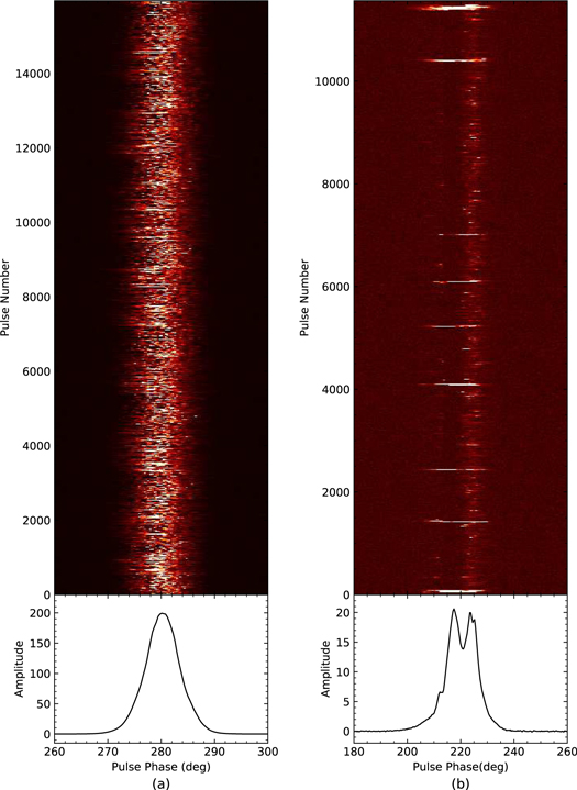
Figure 1. The grayscale intensities of all the single pulse sequences observed in both pulsars: (a) PSR J0614+2229; (b) PSR J1938+2213. In the lower part of the figure, the average pulse profiles are shown.
Download figure:
Standard image High-resolution image
Figure 2. The sequence of subintegrations, each averaged over 30 individual pulses, of PSR J0614+2229. The right-hand panel shows the pulse energy variations for the sequence throughout the on-pulse window, where the red and blue lines represent state A and state B, respectively.
Download figure:
Standard image High-resolution image
Figure 3. Histogram of the Δχ2 for the subintegration data of PSR J0614+2229. In which, the vertical black dashed line represents the threshold based on the combination of two Gaussian components (red dotted lines) that distinguishes the two states.
Download figure:
Standard image High-resolution imageWe measured an RM of 66.84 ± 0.02 rad m−2 for PSR J0614+2229, which is more accurate than the psrcat value of 66.0 ± 0.3 rad m−2 (Johnston et al. 2007). The Faraday rotation effect in our data has been corrected by using 66.84 rad m−2. The polarization profiles of the two states are shown as the red (state A) and blue (state B) lines in subplot (a) of Figure 4. The peak flux density of state A is 204.945 mJy, which is slightly smaller than that of state B of 207.527 mJy. This is consistent with the results at 1400 MHz of Seymour et al. (2014). We estimated the fractional linear polarization by calculating the ratio between the mean linear polarization intensity 〈L〉 and the mean flux density S. The fractional linear polarization (〈L〉/S) for state A is 69.60%, which is smaller than that for state B of 85.32%. The fractional circular polarization (〈V〉/S) for state A is 19.28%, which is larger than that of state B of 13.49%. The absolute circular polarization fraction (〈∣V∣〉/S) for states A and B are 19.28% and 13.51%, respectively. The 〈L〉/S, 〈V〉/S, and 〈∣V∣〉/S for the average profile of PSR J0614+2229 are 75.17%, 17.16%, and 17.16% at 1250 MHz, respectively. By comparing the polarization results that obtained at about 325 and 610 MHz (Olszanski et al. 2019; Mitra et al. 2016), we find that PSR J0614+2229 shows decreasing fractional linear polarization and increasing fractional circular polarization with increasing frequency, like most of pulsars (Sobey et al. 2021). The PA swings of the average profile of the two states are also different. The profile of state A is slightly earlier than that of state B in longitude. The offset of the profile peaks between the two emission states is about 105 in our data. The profile of state A is slightly wider than that of state B. The profile widths of states A and B at the peak intensity levels of 10% are 1477 ± 035 and 1336 ± 035, while at the peak intensity level of 50%, the profile widths of states A and B are 703 ± 035 and 668 ± 035, respectively.
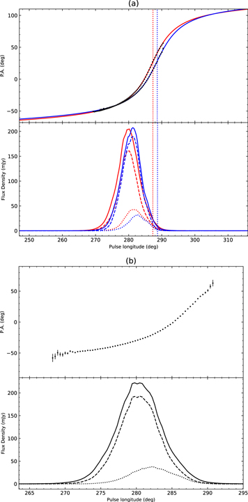
Figure 4. Subplot (a): average polarization properties of state A (red lines) and state B (blue lines). Subplot (b): average polarization properties of the AB-bright phase (see the text for details). The lower panels in each subplot show the pulse profiles for total intensity (solid line), linearly polarized intensity (dashed line), and circularly polarized intensity (dotted line). The S-shaped solid lines in the upper panel of subplot (a) represent the best fits of the PA swings. The vertical dotted lines show the steepest gradient point phase of the RVM fit, ϕ0.
Download figure:
Standard image High-resolution imageAs shown in Figure 2, the emissions of PSR J0614+2229 become much brighter during the transition between the two states. The red and blue lines in the right panel of Figure 2 indicate state A and state B, respectively. These brighter subintegrations are detected in both states. To further study these brighter subintegrations, we selected subintegration sequences belonging to each state whose durations are longer than four subintegrations. The first two and last two pulses of each sequence were folded to construct an average pulse profile for the mode transition phases, namely the AB-bright phase. The average polarization profile for the AB-bright phase is shown in the subplot (b) of Figure 4. Just as expected, the profile of the AB-bright phase is brighter than that of both state A and state B. The peak flux density of the AB-bright phase is 222.08 mJy, which is 17.13 mJy larger than that of state A and is 14.55 mJy larger than that of state B. The W10 of the AB-bright phase is 1406 ± 035, which falls in between that of state A and state B. The W50 of the AB-bright phase is 703 ± 035, which is equal to that of state A, but larger than that of state B. The 〈L〉/S, 〈V〉/S, and 〈∣V∣〉/S of the AB-bright phase are 78.60%, 15.47%, and 15.49%, respectively, which are all fall in between that of state A and state B. The PA swings of the state A, state B, and AB-bright phase are shown in Figure 5. The PA swings of state A (red line) and state B (blue line) exhibit different variations. The PA curve of the AB-bright phase (black line) lies between that of state A and state B, but closer to state B. Our results suggest that the emissions of the two states of PSR J0614+2229 may be generated in different regions in the pulsar magnetosphere. The AB-bright emission may be generated in the region that lies between state A and state B.

Figure 5. Changes in the PAs of the linear polarization for PSR J0614+2229 in the state A, state B, and AB-bright phase.
Download figure:
Standard image High-resolution imageThe PA variation of a pulsar usually exhibits an S-shaped sweep through the profile, which has been reported in numerous earlier studies (e.g., von Hoensbroech & Xilouris 1997). In our observations, high signal-to-noise ratio profiles are obtained for states A and B. Using the PSRMODEL plug-in in the PSRCHIVE package, we fitted the PA swings for both states and found that the χ2 value of the fitting of state B is smaller than that of state A. Therefore, we refitted the PA swing of state A with the same α and β values as state B, where α is the angle between the rotation axis and the magnetic axis and β is the angle between the rotation axis and the observers line of sight. We perform Markov Chain Monte Carlo fitting (Johnston & Kramer 2019) using the python package EMCEE (Foreman-Mackey et al. 2013) to determine the values for the steepest point phases (ϕ0) and PA offset (ψ0) of different states. The ϕ0 of states A and B are  ° and
° and  ° at the 16 and 84 percentiles of the distribution, respectively, which are significantly different. The fitting results of the two states are shown in subplot (a) of Figure 4, in which the red and blue curves represent state A and state B, respectively, and the fitted parameters are shown in Table 1.
Table 1. List of the PA-fitting Parameters of PSR J0614+2229
| α | β | ϕ0 | ψ0 | ||
|---|---|---|---|---|---|
| (°) | (°) | (°) | (°) | ||
| J0614+2229 | State A | 44.84 | −3.78 |

|

|
| State B | 44.84 | −3.78 |

|

|
Note. α is the angle between the rotation axis and the magnetic axis, β is the angle between the rotation axis and the observers line of sight, and ψ0 and ϕ0 are the PA and pulse phase of the steepest gradient point of S-shape curve, respectively. δ ϕ0 is the phase difference between the steepest gradient points traversed by PA in different states.
Download table as: ASCIITypeset image
The steepest gradient (SG) point of the PA traverse lies toward on the trailing edges of the profiles due to the aberration retardation effects (Blaskiewicz et al. 1991; Johnston & Weisberg 2006; Mitra & Rankin 2011). By considering the aberration retardation effects, Blaskiewicz et al. (1991) estimated the emission height of PSR J0614+2229 to be 350 ± 100 km at 1.4 GHz. Note that the model presented by Blaskiewicz et al. (1991) works well if there is a full S-shape swing of the PA and the SG is somewhere in the middle of a pulsar window (see, e.g., Rahaman et al. 2021). For PSR J0614+2229, the SG point is supposed to be at the trailing edge of the pulse window and the S-shape swing is not full. Therefore, the emission heights may be not constrained well. However, considering the signal-to-noise ratio of PSR J0614+2229 in our observation is much larger than that of Blaskiewicz et al. (1991), we try to reestimate the emission heights of different states of PSR J0614+2229. The emission height difference between the two states of the pulsar can be estimated from the phase difference (δ ϕ0) between the SG point of their PA traverses (Blaskiewicz et al. 1991): Δhem = Pc δ ϕ0/8π, where c is the speed of the light and P is the rotation period of a pulsar. Using the parameters in Table 1, we obtained that the derived altitude difference between states A and B for PSR J0614+2229 is ∼90 km. Note that there may be a large uncertainty in the value.
3.1.2. Microstructure
Pulsar radiation is characterized by short timescales of about several microseconds to a few hundred microseconds (Craft et al. 1968; Hankins 1972), called microstructures. The microstructure is an important characteristic of pulsar radiation, which is closely related to the emission process (Buschauer & Benford 1980; Lange et al. 1998). Therefore, it can promote or restrict the emission model. Microstructures have not been reported in PSR J0614+2229 up to now. In our observations, the microstructures of single pulses for this pulsar are detected. According to Johnston et al. (2001), the R parameter can be used for the identification of giant micropulse, in which  , where MAXi
, σi
, and mi
are the maximum intensity, the rms, and the mean intensity in the ith bin, respectively. We identified three pulses with R > 20, and the maximum value of R is 21.77. These three single pulses are shown in the upper panel of Figure 6. The brightest of these pulses (the red line) has a peak flux density of 1659.85 mJy, which is 8.32 times stronger than that of the mean pulse profile, and 19.73 times stronger than the mean flux density at that specific pulse phase. We performed an analysis of the microstructure emission timescales (Pμ
) using the method of Mitra et al. (2015). The estimated Pμ
of the three brightest giant micropulses of PSR J0614+2229 are ∼2.0, 2.9, and 2.9 ms using a smoothing bandwidth 0.075.
, where MAXi
, σi
, and mi
are the maximum intensity, the rms, and the mean intensity in the ith bin, respectively. We identified three pulses with R > 20, and the maximum value of R is 21.77. These three single pulses are shown in the upper panel of Figure 6. The brightest of these pulses (the red line) has a peak flux density of 1659.85 mJy, which is 8.32 times stronger than that of the mean pulse profile, and 19.73 times stronger than the mean flux density at that specific pulse phase. We performed an analysis of the microstructure emission timescales (Pμ
) using the method of Mitra et al. (2015). The estimated Pμ
of the three brightest giant micropulses of PSR J0614+2229 are ∼2.0, 2.9, and 2.9 ms using a smoothing bandwidth 0.075.

Figure 6. Three brightest individual pulses showing microstructure. Upper panel: PSR J0614+2229; Lower panel: PSR J1938+2213. For comparison, the average pulse profiles with peak fluxes of 199.28 mJy (PSR J0614+2229) and 20.69 mJy (PSR J1938+2213) are shown by black lines.
Download figure:
Standard image High-resolution image3.2. PSR J1938+2213
3.2.1. Two Emission States
In the right subplot of Figure 1, we showed the single pulse stack and average pulse profile of PSR J1938+2213. It is noticeable that the emission of the pulsar consists of a weak state superposed by brighter bursts, and the weak emission is always present, which is consistent with the results of Lorimer et al. (2013). This suggests that the emissions for the two states may be generated in different regions in the pulsar magnetosphere. These bright pulses show dramatic variations, where the pulse energy can vary up to 57 times larger than the average pulse energy, and the peak flux density of the burst state is 857.8 mJy, which is about 41 times larger than that of the mean pulse profile. The pulse energy is calculated by summing the intensities within the on-pulse window after subtracting the baseline noise.
We named these bright single pulses the burst state. To identify whether the burst state exists in any particular pulse, we used the same method as in Section 3.1.1. If the Δχ2 of an individual pulse is smaller than 410 (the vertical black dashed line in Figure 7), we classify it as the burst state. We found that 271 pulses in PSR J1938+2213 were in burst state, with the duration ranging from 1 to 63 spin periods (0.166 to 379.5 s).
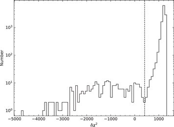
Figure 7. Histogram of Δχ2 for the entire data set of PSR J1938+2213; the vertical black dashed line represents the thresholds for different states.
Download figure:
Standard image High-resolution imageUsing the RMFIT program of PSRCHIVE, the RM we measured for this pulsar is 142.67 ± 0.07 rad m−2 and the Faraday rotation effect has been corrected in our data. The polarization profiles of the two states are shown in Figure 8. The average profile of the weak state (blue line) has two main separated components in which the second component shows two peaks and is much stronger than the first component. The average profile of the burst state (red line) has three main components (separated by the vertical dashed lines in Figure 8) with a stronger central component. The peak flux density of the burst state is about 56 times that of the weak state. The polarization properties of the two states are also different. The 〈L〉/S of the weak state is about 91.33%, which is much larger than that of the burst state of 46.80%. The 〈V〉/S of the weak state is 11.19%, which is also larger than that of the burst state of 1.33%.

Figure 8. Polarization profiles of PSR J1938+2213 for the burst (red lines) and weak (blue lines) states. See Figure 4 for details. The two vertical lines show the longitudes of the orthogonal PA jumps. The dots with error bars in the upper panel are the PAs of the linear polarization for the burst (red) and weak (blue) states.
Download figure:
Standard image High-resolution imageThe PA swings of the two states of PSR J1938+2213 show remarkable differences (the red and blue dots with error bars in the upper panel of Figure 8). The PA swing of the weak state profile shows a smooth variation. The PA swings of the first and third components of the burst state profile basically overlap with the PA curve of the weak state, while PA of the second component shows a sudden jump of about 90◦ (labeled by the vertical dashed lines in Figure 8), known as the orthogonal polarization mode (OPM) phenomenon. Surprisingly, the OPM is not present in the weak state.
We then separated the OPMs for the average profile of the burst state. We assumed that the observed Stokes I, Q, U, and V are the incoherent sum of the 100% polarized OPMs. The two orthogonal modes should have opposite senses of circular polarization. Using the method presented by Karastergiou et al. (2003), we decomposed the average profile of burst state and the mode-separated pulses profiles are shown in Figure 9, in which the positive values of V are associated with Mode 1, and negative V with Mode 2. These two orthogonal polarization modes have PAs separated by 90◦ and each mode is almost completely linearly polarized.

Figure 9. The average pulse profiles of the decomposed orthogonal polarization modes of PSR J1938+2213. The total intensity I, linear polarization L, and circular polarization V of each profile in the lower panels are represented by the black solid, red dotted, and blue dashed lines, respectively. The upper panels give the PAs.
Download figure:
Standard image High-resolution image
3.2.2. Microstructure
The microstructures of single pulses were also detected in PSR J1938+2213. As presented in Section 3.1.2, R is an important parameter for the identification of giant micropulse. We estimated the value of R for PSR J1938+2213, and the measured maximum R is 39.45. There are 41 pulses with R > 25. Three individual pulses with R > 37 are shown in the lower panel of Figure 6. The peak flux density of the brightest pulses (the red line) is 2372.54 mJy, whose peak flux density is about 115 times larger than that of the average pulse at the specific pulse phase. The Pμ of the three brightest giant micropulses of PSR J1938+2213 are ∼1.6, 2.6, and 2.9 ms. As suggested by Mitra et al. (2015), Pμ increases with increasing pulsar spin period, although a large spread of Pμ values exists for all pulsars. Our results basically agree with the conclusion of Mitra et al. (2015).
4. Discussion and Conclusions
We studied the emission variation properties of two pulsars, PSR J0614+2229 and PSR J1938+2213, using the FAST. The highly sensitive observations enable us to study their polarization properties. We found that the emission of PSR J0614+2229 shows two different states, in which the emission of state A occurs earlier than state B in longitude. The phase offset of the profile peaks between the two states is about 105. The PA swings of the two states for PSR J0614+2229 show different variations. PSR J1938+2213 also exhibits two different states: a weak state that is always present and a burst state with dramatic pulse intensity variations. The maximum pulse energy in the burst state is about 57 times larger than the average pulse energy. The PA swings for the two states of PSR J1938+2213 also show different variations.
The PA across the pulse phase (ϕ) was first described by Blaskiewicz et al. (1991) and has later been modified by Dyks (2008) as

where ζ = α + β, r is the radiation height, c is the speed of light, and ϕf is fiducial pulse phase corresponding to the plane containing the rotation and magnetic axis. The changes of emission heights or magnetosphere geometries will result in changes of the PA swing. For PSR J0614+2229, the duration of either state is only about several minutes and the magnetosphere geometry of the pulsar is unlikely to switch between two different states in such short timescales. We attributed the mode changing of this pulsar to the changes in emission heights.
The remarkable feature of PSR J0614+2229 is that the emissions become much brighter during the transition of the two states. This phenomenon has never been seen in other mode-changing pulsars before. These bright subintegrations are named the AB-bright phase. As expected, the average profile of the AB-bright phase is brighter than the profiles of both state A and state B. The radiation height of the AB-bright phase is between the radiation heights of state A and state B, which may be related to the trigger mechanism of mode changing. Similarly, some nulling pulsars show a gradual fall in pulse intensity before the onset of null states, such as PSR J1819+1305 (Rankin & Wright 2008), PSR J1738−2330 (Gajjar et al. 2014), PSR J1502−5653 (Li et al. 2012), and PSR J1752+2359 (Lewandowski et al. 2004; Gajjar et al. 2014; Sun et al. 2021). Gajjar et al. (2014) suggested that the change of states of PSR J1752+2359 may be related to the global magnetospheric change and the gradual fall in pulse intensity may represent a reset or relaxation of the magnetosphere conditions.
For PSR J1938+2213, the weak state is always present, while the burst emission appears superposed over the weak state. The polarization properties of the two states are also different. Our results suggest that the emissions of two states are also generated in different regions in the pulsar magnetosphere. The similar phenomenon has been detected in a double neutron star system PSR B1534+12 (Wang et al. 2020a), in which the weak emission, superposed by bright bursts, is always present. The profile of the burst state of PSR B1534+12 is much narrower than that of the weak state. However, the profiles of weak and burst states for PSR J1938+2213 have a similar width with the overall widths (3σ) of 3902 ± 035 and 4078 ± 035, respectively.
The remarkable feature of PSR J1938+2213 is that the OPM phenomenon is only seen in the burst state. This implies that the burst state is generated in a different region in the pulsar magnetosphere compared to the weak state. Therefore, the plasma environment of the two states may be different, which may result in the OPM only appearing in the burst state. Karastergiou et al. (2011) reported the appearance of a bright additional component in the leading edge of the pulse profile of PSR J0738−4042 with the OPM. By simulation, they concluded that the polarization profiles with the additional component are direct observations of adding an orthogonal polarization mode to the normal profile. Therefore, this additional component may be generated in a region that differs from the normal emission of PSR J0738−4042. Another case is that the OPM appears in all emission states of pulsars, such as PSR B1944+17 (Kloumann & Rankin 2010). PSR B1944+17 shows four different emission states and they all may be generated in a similar region, and thus have a similar emission environment.
According to the RS75 model (Ruderman & Sutherland 1975), the formation of charged bunches can excite coherent curvature radiation along a curved magnetic fields with the characteristic frequency of νc
∼ γ3
c/ρc
(Mitra et al. 2009; Melikidze et al. 2000; Gil et al. 2004; Mitra 2017), where γ is the Lorentz factor of the radiating plasma, ρc
is the underlying radius of curvature, and c is the speed of light. The power of the radio emission is  , where F(Q) is related to the plasma properties in the IAR of the pulsar magnetosphere (Basu et al. 2017). For some mode-changing pulsars, the PA swings of different states show similar variations and the emission heights of different states are similar. In this type of mode-changing pulsar, the emission geometry and emission height remain unchanged in different states; the changes of F(Q) will result in the emission variations, such as PSR J1822−2256 (Basu & Mitra 2018) and PSR J1048−5832 (Yan et al. 2020). However, the origin of the external triggering mechanism that is required to drive the plasma variations in the IAR is unknown (Basu & Mitra 2018, 2019). Recently, Geppert et al. (2021) suggested that the perturbations in the magnetic field that result from Hall and thermal drift oscillations will change the sparking configurations in the IAR, and result in a mode-changing phenomenon. More samples of mode-changing pulsars with high-sensitivity polarimetric observations are required.
This work made use of the data from the FAST telescope (Five-hundred-meter Aperture Spherical radio Telescope). FAST is a Chinese national megascience facility, built and operated by the National Astronomical Observatories, Chinese Academy of Sciences. This work is supported by the West Light Foundation of Chinese Academy of Sciences (WLFC 2021-XBQNXZ-027), the Key Laboratory of Xinjiang Uygur Autonomous Region No. 2020D04049, the National Natural Science Foundation of China (NSFC) project (No. 12041303, 12041304), the National SKA Program of China No. 2020SKA0120200, and the CAS Jianzhihua project. The research is partly supported by the Operation, Maintenance and Upgrading Fund for Astronomical Telescopes and Facility Instruments, budgeted from the Ministry of Finance of China (MOF) and administrated by the CAS, and Guizhou Provincial Science and Technology Foundation (Nos. ZK[[2022]304). Sponsored by Natural Science Foundation of Xinjiang Uygur Autonomous Region (No. 2022D01B71). We thank the reviewer for useful comments.
Software: DSPSR (van Straten & Bailes 2011), PSRCHIVE (Hotan et al. 2004).