


Abstract
We present high-cadence optical, ultraviolet (UV), and near-infrared data of the nearby (D ≈ 23 Mpc) Type II supernova (SN) 2021yja. Many Type II SNe show signs of interaction with circumstellar material (CSM) during the first few days after explosion, implying that their red supergiant (RSG) progenitors experience episodic or eruptive mass loss. However, because it is difficult to discover SNe early, the diversity of CSM configurations in RSGs has not been fully mapped. SN 2021yja, first detected within ≈ 5.4 hours of explosion, shows some signatures of CSM interaction (high UV luminosity and radio and x-ray emission) but without the narrow emission lines or early light-curve peak that can accompany CSM. Here we analyze the densely sampled early light curve and spectral series of this nearby SN to infer the properties of its progenitor and CSM. We find that the most likely progenitor was an RSG with an extended envelope, encompassed by low-density CSM. We also present archival Hubble Space Telescope imaging of the host galaxy of SN 2021yja, which allows us to place a stringent upper limit of ≲ 9 M☉ on the progenitor mass. However, this is in tension with some aspects of the SN evolution, which point to a more massive progenitor. Our analysis highlights the need to consider progenitor structure when making inferences about CSM properties, and that a comprehensive view of CSM tracers should be made to give a fuller view of the last years of RSG evolution.
1. Introduction
Mass loss in massive stars (MZAMS ≳ 8 M☉) is among the most poorly understood aspects of stellar evolution (Smith 2014), and core-collapse supernovae (CCSNe) provide a complementary window into studying mass-loss processes that the stars of the Milky Way and its satellites cannot provide. In the case of pre-SN mass loss, the difficulty lies in the fact that mass-loss rates may change quickly, in which case the SN must be observed very shortly after explosion in order to map out the prognenitor's mass-loss history. For this reason, CCSNe in nearby galaxies—where early discovery, dense time sampling, and rich multiwavelength data sets are possible—offer a valuable opportunity for a mass-loss case study.
Type II supernovae (SNe II), 47 the most common CCSNe (Li et al. 2011; Smith et al. 2011), are the hydrogen-rich explosions of red supergiant (RSG) stars. This has been confirmed by the direct detection of tens of SN II progenitors in archival Hubble Space Telescope (HST) imaging (Smartt 2015; Van Dyk 2016). Traditionally, RSGs were not thought to produce detectable amounts of CSM, but recent work has shown that CSM is nearly ubiquitous in SN II progenitors and can affect the SN observables, particularly during the first days to weeks after explosion. For example, very early spectroscopy has revealed narrow emission lines from high-ionization states, interpreted as forming in the excited but unshocked CSM (Gal-Yam et al. 2014; Smith et al. 2015; Khazov et al. 2016; Yaron et al. 2017; Bullivant et al. 2018; Hosseinzadeh et al. 2018; Soumagnac et al. 2020; Bruch et al. 2021; Hiramatsu et al. 2021b; Terreran et al. 2022). Khazov et al. (2016) and Bruch et al. (2021) have observed these in a large fraction of SNe II. Likewise, Morozova et al. (2017, 2018) show through radiation-hydrodynamical modeling that early SN II light curves require a CSM component to reproduce the fast rise and sometimes even an early peak (see also González-Gaitán et al. 2015; Förster et al. 2018).
Given that both of these CSM signatures disappear shortly after explosion, early discovery, classification, and follow-up are critical to understanding circumstellar interaction in CCSNe, and therefore to understanding mass loss in CCSN progenitors. Specialized surveys like the Distance Less Than 40 Mpc (DLT40) Survey (Tartaglia et al. 2018) observe nearby galaxies frequently (twice per day for DLT40 in the southern hemisphere) with the goal of discovering new transients shortly after explosion, when they are still very faint, and announce discoveries immediately so that spectroscopic classification can occur shortly after. Such projects, used in concert with wide-field transient searches such as the Asteroid Terrestrial-impact Last Alert System (ATLAS; Tonry et al. 2018b), the Young Supernova Experiment (YSE; Jones et al. 2021), the All-Sky Automated Survey for Supernovae (Shappee et al. 2014), and the Zwicky Transient Facility (Bellm et al. 2019), can place strong limits on the explosion epochs of nearby SNe and allow for the most comprehensive early data sets to be acquired. Likewise, rapid robotic follow-up with facilities like Las Cumbres Observatory (Brown et al. 2013) and the Neil Gehrels Swift Observatory (Gehrels et al. 2004) allow us to trace the SN ejecta in detail as it collides with and overruns the material ejected in the years before explosion.
Here we consider the case of SN 2021yja, a nearby (D ≈ 23 Mpc) SN II observed within hours of explosion and followed extensively in the optical and ultraviolet (UV) for the first 150 days of its evolution. The site of SN 2021yja was previously observed with HST to a depth that allows us to place a very strong constraint on the progenitor luminosity. In Section 2, we describe the discovery and observations of SN 2021yja and derive the properties of its host galaxy required for our analysis. In Section 3, we analyze the light curves, spectra, and pre-explosion imaging of SN 2021yja in order to constrain its progenitor properties, including the presence of any CSM, and we compare it to other well-observed SNe II in the literature. Finally, in Section 4, we discuss the implications of our measurements for the population of SN II progenitors and RSGs in general, with a focus on mass-loss histories.
2. Observations and Data Reduction
2.1. Discovery and Classification
SN 2021yja was discovered by ATLAS on 2021-09-08.55 (all dates are in UTC) at c = 15.334 ± 0.007 mag and was not detected on 2021-09-06.48 to a 3σ limit of o > 19.22 mag (Smith et al. 2021; Tonry et al. 2021). Its J2000 coordinates, as measured by Gaia Photometric Science Alerts, are α = 03h24m21 180, (Hodgkin et al. 2021), 99'' southwest of the center of its host galaxy, NGC 1325.
48
It was recovered in earlier unfiltered (357–871 nm) imaging by the DLT40 Survey on 2021-09-08.29 at 16.431 ± 0.028 mag and was not detected on 2021-09-07.28 to a 3σ limit of 18.671 mag. Kilpatrick (2021) also recovered it at g = 20.4 ± 0.2 mag and r = i = 20.7 ± 0.2 mag in publicly available imaging taken on 2021-09-07.63 with the Multicolor Simultaneous Camera for Studying Atmospheres of Transiting Exoplanets 3 (MuSCAT3) on Las Cumbres Observatory's 2 m Faulkes Telescope North (Narita et al. 2020), taken as part of the Faulkes Telescope Project's education and public outreach program.
49
The very low luminosities implied by these magnitudes meant that it was not clear in real time whether these MuSCAT3 images were taken before or after explosion (see Section 3.2).
180, (Hodgkin et al. 2021), 99'' southwest of the center of its host galaxy, NGC 1325.
48
It was recovered in earlier unfiltered (357–871 nm) imaging by the DLT40 Survey on 2021-09-08.29 at 16.431 ± 0.028 mag and was not detected on 2021-09-07.28 to a 3σ limit of 18.671 mag. Kilpatrick (2021) also recovered it at g = 20.4 ± 0.2 mag and r = i = 20.7 ± 0.2 mag in publicly available imaging taken on 2021-09-07.63 with the Multicolor Simultaneous Camera for Studying Atmospheres of Transiting Exoplanets 3 (MuSCAT3) on Las Cumbres Observatory's 2 m Faulkes Telescope North (Narita et al. 2020), taken as part of the Faulkes Telescope Project's education and public outreach program.
49
The very low luminosities implied by these magnitudes meant that it was not clear in real time whether these MuSCAT3 images were taken before or after explosion (see Section 3.2).

SN 2021yja was initially classified as a young SN II by Pellegrino et al. (2021) using a spectrum taken by the Global Supernova Project (GSP) on 2021-09-09.51, 15 hours after the ATLAS discovery report. Their classification was based on spectroscopic comparisons with other SNe II using Superfit (Howell et al. 2005) and the Supernova Identification code (SNID; Blondin & Tonry 2007). Shortly afterward, it was reclassified as a young stripped-envelope SN by Williamson et al. (2021) using a second spectrum taken by the GSP on 2021-09-09.60. They argued that the spectrum also resembled other young SN Ic spectra, and that the putative high-velocity Hα line could have been misidentified silicon 635.5 nm. Several days later, after stronger hydrogen lines had developed, Deckers et al. (2021a, 2021b) restored the SN II classification using a spectrum taken on 2021-09-14.31 by the advanced extended Public ESO Spectroscopic Survey of Transient Objects (ePESSTO+; Smartt et al. 2015).
2.2. Follow-up Photometry and Spectroscopy
We obtained UV, optical, and infrared photometry of SN 2021yja using the Sinistro cameras on Las Cumbres Observatory's network of 1 m telescopes (Brown et al. 2013), 50 MuSCAT3 on Las Cumbres Observatory's 2 m Faulkes Telescope North (Narita et al. 2020), an Andor iKON-L 936 BV camera on the 0.7 m telescope at Thacher Observatory (Swift et al. 2022), KeplerCam on the 1.2 m telescope at F. L. Whipple Observatory (Szentgyorgyi et al. 2005), the Lulin Compact Imager on the 1 m telescope at Lulin Observatory, the MMT and Magellan Infrared Spectrograph (MMIRS) on the MMT (McLeod et al. 2012), the Direct Imaging Camera on the Nickel Telescope (Stone & Shields 1990), the Ultraviolet/Optical Telescope on Swift (Roming et al. 2005), and Andor Apogee Alta F47 cameras on the Panchromatic Robotic Optical Monitoring and Polarimetry Telescopes at Cerro Tololo Inter-American Observatory and Meckering Observatory (Reichart et al. 2005) as part of the DLT40 Survey. See Appendix A for details of the photometry reduction. We also include publicly available photometry from the ATLAS forced photometry server (Tonry et al. 2018a; Smith et al. 2020) and the Supernova Observations and Simulations group (Martinez et al. 2021). Figure 1 shows the light curve of SN 2021yja; the data are available in machine-readable format in the online journal.

Figure 1. The main figure (right) shows the multiband UV-optical-infrared light curve of SN 2021yja through the end of its plateau. Phase is given in rest-frame days after estimated explosion. Note the unusually long ( ≈ 140 days) plateau and slow fall onto the radioactive-decay-powered tail (the last 3 epochs). The inset (left) shows the light curve within 48 hours of explosion, with no filter offsets. In particular, note the MuSCAT3 data (plus signs), which constrains the explosion epoch even more tightly than the nondetections by ATLAS and DLT40 (see Section 3.2).(The data used to create this figure are available.)
Download figure:
Standard image High-resolution imageIn addition, we obtained high-resolution follow-up imaging with the Gemini South Adaptive Optics Imager (GSAOI) at Cerro Pachón, Chile (McGregor et al. 2004). We observed the site of SN 2021yja on 2021-12-18 in H-band using an on-off pattern for 300 s of total on-source exposure. Following procedures in Kilpatrick et al. (2021), we performed image calibration using dark and flat-field frames obtained in the instrumental configuration.
After classification, we initiated a high-cadence optical spectroscopic follow-up campaign using the FLOYDS instruments on Las Cumbres Observatory's 2 m Faulkes Telescopes North and South (FTN & FTS; Brown et al. 2013), Binospec on the MMT (Fabricant et al. 2019), the Wide Field Spectrograph (WiFeS) on the 2.3 m telescope at Siding Spring Observatory (SSO; Dopita et al. 2007, 2010), the ESO Faint Object Spectrograph and Camera 2 (EFOSC2) on the New Technology Telescope (NTT; Buzzoni et al. 1984); the Keck Cosmic Web Imager (KCWI) on Keck II (Morrissey et al. 2018), the Robert Stobie Spectrograph (RSS) on the South African Large Telescope (SALT; Smith et al. 2006), the Kast Spectrograph on the Shane Telescope (Miller & Stone 1994), the Boller & Chivens Spectrograph (B&C) on the Bok Telescope (Green et al. 1995), the High-Resolution Echelle Spectrometer (HIRES) on Keck I (Vogt et al. 1994), the Goodman High Throughput Spectrograph on the Southern Astrophysical Research Telescope (SOAR; Clemens et al. 2004), and the Dual Imaging Spectrograph (DIS) on the Astrophysical Research Consortium (ARC) 3.5 m telescope (Lupton 2005). Figure 2 compares the earliest spectra of SN 2021yja, taken within 6 days of estimated explosion, to other early spectra of SNe II from Yaron et al. (2017); Andrews et al. (2019); Hiramatsu et al. (2021b); Tartaglia et al. (2021), and Terreran et al. (2022). The remaining optical spectra are plotted in Figure 3. We also obtained near-infrared spectra using the Near-Infrared Echelette Spectrometer (NIRES) on Keck II (Wilson et al. 2004), the Son of ISAAC spectrograph (SOFI) on the NTT (Moorwood et al. 1998), TripleSpec 4.1 on SOAR (Schlawin et al. 2014), and MMIRS on the MMT, which are plotted in Figure 4. All spectra were either observed at the parallactic angle, or an atmospheric dispersion corrector was used. Details of the spectroscopic reductions are given in Appendix B.

Figure 2. The early spectroscopic evolution of SN 2021yja compared to several other SNe II with good explosion constraints. The labels to the right of each spectrum give phase in rest-frame days after explosion, with uncertainties of 0.1–0.5 days. SN 2021yja does not show strong, narrow high-ionization lines like SNe 2013fs, 2017ahn, 2018zd, and 2020pni, an indication of short-lived circumstellar interaction. However, it does show broader features, including a mysterious broad feature around 450 nm (labeled "ledge") denoted by a gray bar, also seen in SN 2017gmr.(The data used to create this figure are available.)
Download figure:
Standard image High-resolution image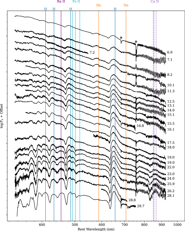
Download figure:
Standard image High-resolution image
Figure 3. The spectroscopic evolution of SN 2021yja > 6 days after explosion, with colored lines at the rest wavelengths of selected features. (The data used to create this figure are available—See Figure 2.)
Download figure:
Standard image High-resolution image
Figure 4. Near-infrared spectra of SN 2021yja. The weak helium absorption and the high-velocity helium feature in our > 100 d spectra indicate that SN 2021yja belongs to the "weak" class of Davis et al. (2019). (The data used to create this figure are available—See Figure 2.)
Download figure:
Standard image High-resolution image2.3. Pre-explosion Imaging
NGC 1325 and the site of SN 2021yja were observed by HST on 1997-03-26 with the Wide Field Planetary Camera 2 (WFPC2) in F606W (PI Stiavelli, SNAP-6359). We reduced all c0m frames with the hst123 reduction pipeline and performed final photometry in the c0m frames using dolphot. In addition, we obtained DECam grizY imaging taken between 2014 and 2019 and covering the site of SN 2021yja. We stacked and calibrated all such data using a custom pipeline based on the photpipe imaging and photometry package (Rest et al. 2005). Finally, we downloaded pre-explosion Spitzer/IRAC imaging (Fazio et al. 2004; Werner et al. 2004; Gehrz et al. 2007) from the Spitzer Heritage Archive and combined the basic calibrated data (cbcd) frames following methods described in Kilpatrick et al. (2021). These pre-explosion data are analyzed in Section 3.5.
2.4. Redshift
NGC 1325 has a heliocentric redshift of z = 0.005307 ±0.000005 (Springob et al. 2005). However, we observe a weak, narrow Hα emission line in our Keck HIRES spectrum at a redshift of z = 0.00568, corresponding to a line-of-sight velocity of cΔz = + 112 km s−1 with respect to the galaxy core. This velocity is reasonable given the position of the SN and a typical galaxy rotation curve (Falcón-Barroso et al. 2017; Guidi et al. 2018), so we adopt this as the SN redshift.
2.5. Extinction
The equivalent widths of Na i D absorption lines have been shown to correlate with extinction due to interstellar dust (Richmond et al. 1994; Munari & Zwitter 1997). In order to measure the extinction in the direction of SN 2021yja, we examine the Na i D features in our Keck HIRES spectrum (pixel scale Δx ≈ 0.0026 nm in the regions of interest), shown in Figure 5. The spectrum reveals four distinct absorption systems at z = 0.00002 (Milky Way), 0.00559, 0.00566, and 0.00568.

Figure 5. A high-resolution spectrum of SN 2021yja in the regions surrounding Na i D and the diffuse interstellar band (DIB) at 578 nm. The colored lines in the left and center panels indicate four distinct line-of-sight absorbers: one in the Milky Way (z = 0.00002) and three in the host galaxy (z = 0.00559, 0.00566, and 0.00568). Applying the relations of Poznanski et al. (2012), the Milky Way component is consistent with E(B − V)MW = 0.0191 mag from the dust maps of Schlafly & Finkbeiner (2011). The strong host galaxy components indicate an additional extinction of mag, which is surprising given the blue observed colors of SN 2021yja. The DIB (right) confirms the significant extinction in the host galaxy. The blue Gaussian is a fit to the data, while the orange Gaussian shows the strength of DIB we would expect given the Na i D absorption, according to the extinction relation of Phillips et al. (2013). We adopt a total extinction of E(B − V) = 0.104 mag. (The data used to create this figure are available—See Figure 2.)

Download figure:
Standard image High-resolution imageWe measure the equivalent widths of each of these eight lines by fitting and integrating a Gaussian profile, resulting in the values shown in Table 1. (For the systems at z = 0.00566 and 0.00568, we simultaneously fit two Gaussian profiles.) We then convert these equivalent widths to E(B − V) using Eq. (9) of Poznanski et al. (2012) and applying the renormalization factor of 0.86 from Schlafly et al. (2010). The Milky Way extinction value, mag, is consistent with the value from Schlafly & Finkbeiner (2011), E(B − V)MW = 0.0191 mag. We adopt the latter. The host galaxy extinction value (from the sum of the six lines) is mag.


Table 1. Equivalent Widths
| Line | Redshift | Wλ (nm) |
|---|---|---|
| DIB | 0.00568 | 0.0076 |
| D2Na i | 0.00002 | 0.0059 |
| D1Na i | 0.00002 | 0.0024 |
| D2Na i | 0.00559 | 0.0134 |
| D2Na i | 0.00566 | 0.0148 |
| D2Na i | 0.00568 | 0.0108 |
| D1Na i | 0.00559 | 0.0111 |
| D1Na i | 0.00566 | 0.0128 |
| D1Na i | 0.00568 | 0.0091 |
Download table as: ASCIITypeset image
This is a surprisingly high value given the already very blue observed colors of SN 2021yja (see Section 3.1). To confirm this measurement, we also measure the equivalent width of the diffuse interstellar band (DIB) at 578 nm. From Equation (6) of Phillips et al. (2013), which can be rewritten

using the extinction law of Schlafly & Finkbeiner (2011), we would expect an equivalent width of nm. Due to the lower signal-to-noise ratio of this feature, we fit a Gaussian with a fixed center (578 nm at z = 0.00568) and width (FWHM = 0.222 nm; Tuairisg et al. 2000). Again integrating the best-fit Gaussian, we get an equivalent width consistent with our expectation, Wλ = 0.0076 nm. Given the more robust detection of the Na i D lines, we adopt the extinction derived above, for a total of E(B − V) = 0.104 mag, for which we correct using the extinction law of Fitzpatrick (1999). Note that this only accounts for interstellar extinction in the host galaxy, and not for any extinction due to CSM.

2.6. Distance
Distance estimates for NGC 1325 based on the method of Tully & Fisher (1977) listed on the NASA/IPAC Extragalactic Database range from 17.7 to 26.1 Mpc (μ = 31.24 − 32.09 mag). For comparison, the redshift-dependent distance of NGC 1325 is 23.6 ± 4.5 Mpc, assuming the cosmological parameters of the Planck Collaboration et al. (2020) and an uncertainty of cz ≈ 300 km s−1 due to the galaxy's peculiar velocity.
As an additional check on the SN distance, we apply the expanding photosphere method (EPM; Kirshner & Kwan 1974), which is a geometrical technique that can independently constrain the distance of an individual Type II SN. Assuming that the SN photosphere is expanding freely and spherically shortly after the explosion, we can derive the distance from the linear relation between the angular radius and the expanding velocity of the photosphere using the function

where D is the distance, vphot and θ are the velocity and angular radius of the photosphere, respectively, and t0 is the explosion epoch. We estimate the photospheric velocity by measuring the minimum of the P Cygni profile of the Fe ii line at 516.9 nm, which becomes detectable ∼ 19 days after explosion. These measurements are listed in Table 2. In practice, the SN photosphere radiates as a dilute blackbody, so a dilution factor has to be involved when determining θ (Eastman et al. 1996; Hamuy et al. 2001; Dessart & Hillier 2005). We combine the multiband photometry to simultaneously derive the angular size (θ) and color temperature (Tc) by minimizing the equation

where ξ and bν are the dilution factor and the synthetic magnitude, respectively, both of which can be treated as a function of Tc (Hamuy et al. 2001; Dessart & Hillier 2005), Aν is the reddening, mν is the observed magnitude, and S is the filter subset, i.e., {B, V}, {B, V, I} and {V, I}. We use the dilution factors calculated by Jones et al. (2009) with the atmosphere model from Dessart & Hillier (2005). The best-fitting parameters D and t0 in Equation (2) are estimated with a Markov Chain Monte Carlo (MCMC) method, and the priors of parameters are assumed to be uniform. The upper bound on the prior of t0 is set to be MJD 59464.63, the first detection of the SN. Jones et al. (2009) showed that there is a clear departure from linearity between θ/v and t ≳ 40 days after explosion. Therefore, only data before this phase are used in our calculations (see Table 2). For the three filter subsets, we obtain distances of Mpc, Mpc, and Mpc, respectively. The explosion epochs are constrained to be d, d, and d, respectively, relative to the estimate from our shock cooling model (see Section 3.2).


Table 2. Data and Results for the Expanding Photosphere Method
| Phase | Fe ii Velocity | B | V | I | BV | BVI | VI | |||
|---|---|---|---|---|---|---|---|---|---|---|
| (d) | (Mm s−1) | (mag) | (mag) | (mag) | θ/v (Mpc−1 d) | Temp. (K) | θ/v (Mpc−1 d) | Temp. (K) | θ/v (Mpc−1 d) | Temp. (K) |
| 19.0 | 8.122 ± 0.389 | 14.733 ± 0.056 | 14.549 ± 0.062 | 14.256 ± 0.045 | 0.805 ± 0.127 | 0.847 ± 0.068 | 0.866 ± 0.123 | |||
| 22.0 | 8.091 ± 0.161 | 14.894 ± 0.061 | 14.582 ± 0.054 | 14.201 ± 0.029 | 0.940 ± 0.100 | 0.990 ± 0.044 | 1.015 ± 0.087 | |||
| 23.0 | 7.747 ± 0.180 | 14.894 ± 0.061 | 14.548 ± 0.063 | 14.192 ± 0.028 | 1.032 ± 0.113 | 1.040 ± 0.047 | 1.028 ± 0.103 | |||
| 24.0 | 7.599 ± 0.161 | 14.901 ± 0.056 | 14.518 ± 0.058 | 14.178 ± 0.027 | 1.105 ± 0.104 | 1.075 ± 0.045 | 1.032 ± 0.100 | |||
| 25.9 | 7.190 ± 0.139 | 15.012 ± 0.090 | 14.605 ± 0.067 | 14.213 ± 0.040 | 1.131 ± 0.136 | 1.153 ± 0.063 | 1.146 ± 0.124 | |||
| 26.2 | 7.264 ± 0.142 | 15.022 ± 0.076 | 14.609 ± 0.066 | 14.210 ± 0.040 | 1.131 ± 0.123 | 1.154 ± 0.059 | 1.145 ± 0.121 | |||
| 28.1 | 7.220 ± 0.138 | 15.049 ± 0.076 | 14.614 ± 0.057 | 14.223 ± 0.037 | 1.159 ± 0.111 | 1.155 ± 0.056 | 1.136 ± 0.109 | |||
| 29.7 | 5.986 ± 0.177 | 15.148 ± 0.073 | 14.643 ± 0.054 | 14.170 ± 0.012 | 1.456 ± 0.125 | 1.505 ± 0.059 | 1.535 ± 0.106 | |||
| 30.1 | 6.719 ± 0.115 | 15.166 ± 0.065 | 14.642 ± 0.054 | 14.169 ± 0.013 | 1.313 ± 0.101 | 1.353 ± 0.037 | 1.368 ± 0.090 | |||
| 31.2 | 6.312 ± 0.111 | 15.240 ± 0.080 | 14.658 ± 0.058 | 14.181 ± 0.018 | 1.439 ± 0.122 | 1.449 ± 0.048 | 1.452 ± 0.104 | |||
| 32.1 | 6.041 ± 0.093 | 15.202 ± 0.076 | 14.625 ± 0.059 | 14.193 ± 0.026 | 1.524 ± 0.126 | 1.485 ± 0.052 | 1.447 ± 0.114 | |||
| 33.9 | 6.093 ± 0.096 | 15.317 ± 0.070 | 14.696 ± 0.056 | 14.131 ± 0.033 | 1.508 ± 0.114 | 1.613 ± 0.054 | 1.670 ± 0.101 | |||
| 37.0 | 5.659 ± 0.089 | 15.401 ± 0.061 | 14.684 ± 0.051 | 14.162 ± 0.029 | 1.734 ± 0.116 | 1.729 ± 0.052 | 1.713 ± 0.102 | |||
| 39.8 | 5.553 ± 0.075 | 15.516 ± 0.067 | 14.757 ± 0.054 | 14.195 ± 0.028 | 1.749 ± 0.125 | 1.766 ± 0.049 | 1.776 ± 0.098 | |||


A machine-readable version of the table is available.
Download table as: DataTypeset image
Seeing that these distances are consistent with the Tully-Fisher distance above, and given the large uncertainties from this method, we adopt the most recent Tully-Fisher estimate (calculated using the I band), Mpc (μ = 31.85 ± 0.45 mag; Tully et al. 2016). However, we keep in mind that all of our luminosity-dependent measurements suffer from a large systematic uncertainty in the distance.

3. Analysis
3.1. Bolometric Light Curve and Colors
For the purposes of constructing a bolometric light curve, we restrict ourselves to epochs where we have Swift observations, as UV photometry is critical for constraining the SED of young SNe. We supplement the Swift photometry with ground-based griz observations taken within 0.5 days of the Swift observation window. We fit a blackbody spectrum to the observed SED at each epoch using an MCMC routine implemented in the Light Curve Fitting package (Hosseinzadeh & Gomez 2020). This gives the temperature and radius evolution in the bottom panel of Figure 6. We then integrate the best-fit blackbody from the blue edge of the U band to the red edge of the I band to produce a pseudobolometric light curve, such that it will be comparable to pseudobolometric light curves in the literature. The top panel of Figure 6 compares the pseudobolometric light curve of SN 2021yja to 39 other SNe II from Valenti et al. (2016). SN 2021yja is among the most luminous.

Figure 6. Top: Pseudobolometric light curve of SN 2021yja (black) compared to a sample of 39 pseudobolometric light curves from Valenti et al. (2016). Bottom: Evolution of the blackbody temperature of SN 2021yja compared to temperature evolution models of Kozyreva et al. (2020). SN 2021yja lies between the models with progenitor radii of 800 R☉ and 1000 R☉, although no model is significantly hotter than SN 2021yja. Note that the blackbody temperature does not cool below the hydrogen recombination threshold ( ∼ 0.7 eV; dotted line) for several weeks, seemingly inconsistent with the appearance of strong hydrogen P Cygni lines after the first few days. This becomes relevant for the validity of our shock cooling model (Section 3.2).(The data used to create this figure are available.)
Download figure:
Standard image High-resolution imageA comparison with the light-curve model grid from Hiramatsu et al. (2021a) suggests that a hydrogen-rich envelope mass ≳ 5 M☉ is required to reproduce the unusually long plateau duration ( ≈ 140 days). A higher explosion energy ( ≳ 2 × 1051 erg) is also likely required to reproduce the plateau luminosity of SN 2021yja, which is higher than the models, suggesting an even more massive hydrogen-rich envelope according to light-curve scaling relations (e.g., Popov 1993; Kasen & Woosley 2009; Goldberg et al. 2019).
As suggested by Rubin & Gal-Yam (2017) and Kozyreva et al. (2020), the temperature evolution prior to the recombination phase can serve as a solid diagnostic of the progenitor radius. The temperature declines as a power law during this period and changes to a shallower decline after the onset of recombination (Nakar & Sari 2010; Shussman et al. 2016; Sapir & Waxman 2017; Faran et al. 2019), making this phase relatively easy to distinguish. In the bottom panel of Figure 6, we compare the temperature evolution of SN 2021yja to temperature models from Kozyreva et al. (2020) for various progenitor radii. We find that SN 2021yja lies between the 800 R☉ and 1000 R☉ models. Although there is no larger/hotter model, this comparison demonstrates that the progenitor of SN 2021yja is at least consistent with typical RSG radii (100 − 1500 R☉; Levesque 2017), in contrast to our findings in Section 3.2.
We also downloaded UV light curves of all SNe II in the Swift Optical/Ultraviolet Supernova Archive (Brown et al. 2014). We correct these for Milky Way extinction only and plot them in Figure 7. SN 2021yja is the second most UV-luminous SN II observed by Swift, after only SN 2020pni (Terreran et al.2022).

Figure 7. The UV light curve of SN 2021yja (shaded gray) compared to all SNe II in the Swift Optical/Ultraviolet Supernova Archive (colored points; corrected for Milky Way extinction only; Brown et al. 2014). All Swift data are in Vega magnitudes. The top of the gray region corresponds to mag, whereas the bottom is only corrected for Milky Way extinction. This makes SN 2021yja the second most UV-luminous SN II observed by Swift, after SN 2020pni (blue octagons; Terreran et al. 2022). This unusually high UV luminosity suggests circumstellar interaction.

Download figure:
Standard image High-resolution imageLastly, in Figure 8, we compare the optical colors of SN 2021yja to a sample of other SNe II (Hamuy et al. 2001; Leonard et al. 2002; Elmhamdi et al. 2003; Bose et al. 2013; Munari et al. 2013; Anderson et al. 2014; Brown et al. 2014; Dall'Ora et al. 2014; Faran et al. 2014; Galbany et al. 2016; Rubin et al. 2016; Hosseinzadeh et al. 2018; de Jaeger et al. 2019; Szalai et al. 2019; Andrews et al. 2019; Bostroem et al. 2020; Dong et al. 2021; Terreran et al. 2022). The evolution is fairly typical, starting near the minimum colors for a hot blackbody, then evolving redward, with an inflection point around 15 days after explosion. In the terminology of Anderson et al. (2014), this is the transition time ttran when the light-curve slope changes from s1 (the initial decline) to s2 (the "plateau"; see their Figure 1). Notably, we observe this transition in the colors even though the bolometric light curve in Figure 6 does not have a significant inflection point. We discuss this further in Section 4.1.

Figure 8. Extinction-corrected color curves of SN 2021yja compared to other SNe II. Open markers for g − r and r − i are converted from V − R and R − I, respectively, according to the relationships of Jordi et al. (2006). The bump in the color curves ending around 15 d happens around the same time that a change in plateau slope is commonly observed in SNe II (Anderson et al. 2014), although such a change is not obvious in our light curve. Otherwise, the color evolution of SN 2021yja is fairly typical.(The data used to create this figure are available.)
Download figure:
Standard image High-resolution image3.2. Shock Cooling Model
In the absence of circumstellar interaction, the early light curves of CCSNe are dominated by shock cooling emission, which depends upon the parameters of the explosion and the progenitor star, in particular the progenitor radius. We fit the model of Sapir & Waxman (2017) to the early light curve of SN 2021yja using the MCMC routine implemented in the Light Curve Fitting package (Hosseinzadeh & Gomez 2020). Because of the large uncertainties in extinction and distance outlined above, we allowed these to be free parameters in our model, with Gaussian priors according to their known values. We also included an intrinsic scatter term, σ, such that the effective uncertainty on each point is increased by a factor of , with a half-Gaussian prior. This allows us to capture additional uncertainties, e.g., from photometric calibration, deviations from a blackbody spectrum, or small variations around the model, in our reported parameter uncertainties. The prior shapes and limits are given in Table 3. We ran 100 walkers for 1000 steps to reach convergence, assessed via visual inspection of the chain history, and for an additional 1000 steps to sample the posterior. Figure 9 shows the best-fit light curve, as well as the posterior distributions of and correlations between each parameter.


Figure 9. Modeling the shock cooling emission of SN 2021yja using the model of Sapir & Waxman (2017). The parameters are described in Table 3. We find that the first detection with MuSCAT3 occurred 5.4 ± 1.4 rest-frame hours after the best-fit explosion time. We also find the best-fit progenitor radius to be . This unusually large radius for an RSG can be lowered if we adopt a smaller extinction value or if we attribute some of the UV flux to interaction with CSM.(The data used to create this figure are available.)

Download figure:
Standard image High-resolution imageTable 3. Shock Cooling Parameters
| Parameter | Variable | Prior Shape | Prior | Parameters a | Best-fit Value b | Units |
|---|---|---|---|---|---|---|
| Shock velocity | vs* | Uniform | 0 | 3 | 1.0 ± 0.2 | 108.5 cm s−1 |
| Envelope mass c | Menv | Uniform | 0 | 10 | 0.6 ± 0.1 | M☉ |
| Ejecta mass × numerical factor d | fρ M | Uniform | 3 | 100 | 60 ± 30 | M☉ |
| Progenitor radius | R | Uniform | 0 | 100 | 14 ± 2 | 1013 cm |
| Distance | dL | Gaussian | 23.4 | 4.9 | 25 ± 5 | Mpc |
| Extinction | E(B – V) | Gaussian | 0.104 | 0.0155 | mag | |
| Explosion time | t0 | Uniform | 59460 | 59464.6 | 59464.40 ± 0.06 | MJD |
| Intrinsic scatter | σ | Half-Gaussian | 0 | 1 | 4.8 ± 0.2 | Dimensionless |

Notes.
a The "Prior Parameters" column lists the minimum and maximum for a uniform distribution, and the mean and standard deviation for a Gaussian distribution. b The "Best-fit Value" column is determined from the 16th, 50th, and 84th percentiles of the posterior distribution, i.e., median ± 1σ. c Sapir & Waxman (2017) define the envelope of an RSG as the region where , where the density follows (we adopt for convective envelopes). d The ejecta mass and density profile do not have a strong effect on the light curve. Therefore this parameter is essentially unconstrained.


Download table as: ASCIITypeset image
Qualitatively, the model fits SN 2021yja reasonably well across all bands. Unlike for several recent SNe II that have a significant peak in their early light curve (see, e.g., Hosseinzadeh et al. 2018), the shock cooling model is able to reproduce the smooth rise to plateau over ∼ 10 days in the reddest bands. The model is nominally valid until MJD 59496.3 (31.7 days after explosion), at which point the temperature drops below 0.7 eV and recombination breaks the assumption of constant opacity (Sapir & Waxman 2017). This phase is roughly consistent with the recombination limit we estimated in Figure 6. However, there are clear hydrogen features in the spectra starting around 10 days, implying that recombination is occurring much earlier than this. For this reason, we do not fit our light curve after maximum light in the reddest bands (i.e., we only fit the data shown in Figure 9). This inconsistency in recombination time is one clue that the physics behind the shock cooling model may not completely describe the data, despite the appearance of a good fit.
Putting this concern aside for the moment, the model is most sensitive to the progenitor radius. The best-fit progenitor radius is , which is significantly larger than typical RSG radii (100 − 1500 R☉; Levesque 2017), and larger than the radius we infer in Section 3.1. Inspecting the correlations in Figure 9, we see that the radius estimate is strongly (positively) correlated with the extinction estimate. In other words, if we decrease our adopted extinction by 1 − 2σ, we would estimate a more reasonable radius. However, we performed a second fit with a uniform prior in E(B − V) and derived a best-fit extinction value similar to that in Section 2.5. (As Sapir & Waxman 2017 assume a blackbody SED in their model, this is equivalent to determining the extinction required to redden a blackbody into the observed SED.) Alternatively, as we discuss further in Section 4.1, the extreme UV flux may be the effect of circumstellar interaction on our light curve, which is not included in the shock cooling model. If we could model this interaction component separately, a smaller radius might be required to generate the shock cooling component. We can treat our best-fit radius as a robust upper limit on the true progenitor radius, though admittedly it is not very constraining.

We also find a best-fit explosion (shock-breakout) time of MJD 59464.40 ± 0.06, a mere 5.4 ± 1.4 rest-frame hours before our serendipitous detection with MuSCAT3. One possibility, first suggested by Kilpatrick (2021), is that this first detection is of the progenitor prior to shock breakout. Indeed the absolute magnitude at this phase (Mr = − 11.5 mag, Mi = − 11.3 mag) is similar to the "precursor emission" of SN 2020tlf observed by Jacobson-Galán et al. (2022). To investigate this possibility, we performed the light-curve fit again without this first detection. The best-fit explosion time is still before the MuSCAT3 detection, and the model has a slightly larger intrinsic scatter (σ ≈ 5.8). In the absence of extraordinary proof to the contrary, we conclude that this detection was after explosion and adopt the explosion time above as phase = 0 throughout our figures.
3.3. Nickel Mass
Near the end of our observations presented here, as of around 138 rest-frame days after explosion, the light curve of SN 2021yja has settled on the radioactive-decay tail, where the 56Co → 56Fe decay provides most of the input power. We confirm that the bolometric decline rate over the last four epochs of photometry from Las Cumbres Observatory is 0.0096 mag day−1, very close to the 56Co → 56Fe decay rate (0.0098 mag day−1; Colgate & McKee 1969). During this phase, we can measure the mass of radioactive 56Ni produced in the explosion by scaling the luminosity to that of SN 1987A, which had an independent 56Ni measurement (MNi,87A=0.075 M☉; Spiro et al. 2014; Valenti et al. 2016).
We calculate the bolometric luminosity for these four epochs by directly integrating the SED over the U to i filters. This is different than the blackbody-fitting method we used during the photospheric phase, because at these late times the SED is no longer described by a Planck (1906) function (e.g., Martinez et al.2022). We calculate a bolometric light curve of SN 1987A with the same method using photometry from Catchpole et al. (1988) via the Open Supernova Catalog (Guillochon et al. 2017), interpolate to the four epochs of SN 2021yja photometry, and take the average ratio. We find that SN 2021yja produced , where the uncertainty is dominated by our distance uncertainty. This places SN 2021yja at the 97th percentile for nickel mass among SNe II (Anderson 2019), although we caution that this measurement is only ≈ 1.6σ above the nickel mass of SN 1987A. Another possibility is that our measurement is inflated by extra luminosity from ongoing circumstellar interaction, although the decline slope we measure above suggests that 56Co decay is the dominant power source. An unusually large nickel mass may suggest a massive progenitor, according to the correlations of Eldridge et al. (2019). We discuss this possibility further in Section 4.2.

3.4. Spectral Features
The spectroscopic evolution of SN 2021yja ≳ 6 days after explosion is typical for a SN II: P Cygni lines of hydrogen and helium superimposed on a cooling blackbody. Metal lines, including Ba ii and Fe ii begin to appear several weeks after explosion, blanketing the blue side of the spectrum. Its infrared spectra (Figure 4) place it in the "weak" class of Davis et al. (2019), with weak helium absorption at 1.083 μm in our > 100 d spectra, a high-velocity component of the same line, and more pronounced Sr ii absorption. As such, SN 2021yja is consistent with the correlation between slow plateau decline rates and weak infrared helium absorption (Davis et al. 2019). No carbon monoxide emission is detected at 100 days after explosion.
However, our earliest optical spectra, taken around 2 days after explosion, are somewhat unusual in the sense that they do not show the narrow high-ionization lines seen in many SNe II this early. These lines indicate short-lived circumstellar interaction, which ends when the nearby circumstellar material (CSM) is swept up by the expanding ejecta (Gal-Yam et al. 2014; Smith et al. 2015; Khazov et al. 2016; Yaron et al. 2017; Bullivant et al. 2018; Hosseinzadeh et al. 2018; Soumagnac et al. 2020; Bruch et al. 2021; Hiramatsu et al. 2021b; Terreran et al. 2022). Figure 2 compares the early spectra of SN 2021yja to other SNe II with well-constrained explosion dates and high-quality spectra taken within 6 days of explosion. Some show narrow He ii, C iii, N iii, and other lines: SN 2013fs (Yaron et al. 2017; Bullivant et al. 2018), SN 2017ahn (Tartaglia et al. 2021), SN 2018zd (Hiramatsu et al. 2021b), and SN 2020pni (Terreran et al. 2022). SN 2017gmr (Andrews et al. 2019) and SN 2021yja do not show these lines, but instead show a unique "ledge-shaped" feature around 450–480 nm, which we discuss below.
Figure 10 shows a detailed view of the ledge-shaped feature in the earliest spectrum of SN 2021yja, compared to Hα and He 587.6 nm in the same spectrum. There are two lines of thought about the identity of this feature in the literature, both related to circumstellar interaction. Bullivant et al. (2018, their Figure 20) and Andrews et al. (2019, their Figure 18) interpret it as very broad, blueshifted He ii 468.6 nm (although there is also a narrow component of this line present) produced in the outermost layers of the SN ejecta. However, the line profile is somewhat more symmetrical in these SNe than in SN 2021yja. Soumagnac et al. (2020, their Figure 7) and Bruch et al. (2021, their Figure 5) interpret this feature as a blend of various flash-ionized lines from the CSM: N v 460.4 and 462.0 nm, N ii 463.1 and 464.3 nm, C iv 465.8 nm, and He ii 468.6 nm.

Figure 10. The profile of the unidentified feature around 450–480 nm (green) in the first spectrum of SN 2021yja, compared to the profiles of Hα (blue) and He 587.6 nm (orange). He ii could be contributing at 468.6 nm, but the feature is broad and has an irregular shape, unlike the other P Cygni profiles. As suggested by Soumagnac et al. (2020) and Bruch et al. (2021), we suspect this is a combination of several lines, possibly indicating a low level of circumstellar interaction. However, its breadth cannot be fully explained by the handful of narrow flash-ionized lines they suggest.
Download figure:
Standard image High-resolution imageNeither of these explanations is fully satisfactory. The former (single, broad line) is difficult to reconcile with the irregular profile of the feature, when other features have typical P Cygni profiles. In addition, the implied velocity is nearly 30,000 km s−1 (as measured from the He ii rest wavelength to the blue edge of the feature), which is much higher than any other feature in the spectrum. The latter explanation (blend of several narrow emission lines) is inconsistent with the breadth and strength of the feature. We suspect that the feature is indeed a blend of several lines, possibly including He ii, C iii, and N iii, although these must be either much broader or much more numerous than the features suggested by previous work. We discuss one such possibility in Section 4.1.
3.5. Limits on a Pre-explosion Counterpart
Figure 11 (left) shows our high-resolution GSAOI image of SN 2021yja, aligned to the pre-explosion WFPC2 F606W image using three common astrometric sources in both frames, resulting in an rms astrometric uncertainty of 0.08'' (0.8 WFPC2 pixels) between both frames. In addition, we aligned the GSAOI image to DECam and Spitzer/IRAC imaging, using 4–6 common astrometric standards in both frames and resulting in an rms uncertainty of 0.07–0.12'' (Figure 11, right).

Figure 11. HST/WFPC2 F606W imaging of NGC 1325 from 1997 colorized using DSS imaging of the same field (left) and showing the explosion site of SN 2021yja (white square). An inset panel shows GSAOI imaging of SN 2021yja obtained in Dec. 2021 in a 40''×40'' region corresponding to the white frame. The right-hand panels show the same region as seen in F606W, DECam grizY, and Spitzer/IRAC Channel 1 and 2, aligned using 3–6 common astrometric standards (blue circles) and centered on the site of SN 2021yja (red circle). The lack of a counterpart is described in Section 3.5.
Download figure:
Standard image High-resolution imageThe position of SN 2021yja does not align with any counterpart in the HST imaging. The closest source is 0.88'' (11σ) away from this position and detected at mF606W = 24.05 ± 0.06 mag (previously discussed in Kilpatrick 2021). The same is true in each of the other pre-explosion images as shown in Figure 11, with no evidence for any significant, point-like emission within at least 3σ of the site of SN 2021yja.
Motivated by the depth of our imaging set, we place 3σ limits on the presence of a counterpart in each of our pre-explosion images. We estimate the standard deviation of the background variation within 2'' of SN 2021yja and use this value to estimate the maximum total flux that would not be flagged as a 3σ detection within one PSF width at this location. The resulting limits are given in AB mag in Table 4, which we consider the 3σ limits on the presence of any counterpart in each image.
Table 4. Limits on a Pre-explosion Counterpart to SN 2021yja
| Instrument | Band | Magnitude |
|---|---|---|
| WFPC2 | F606W | >27.15 |
| DECam | g | >24.50 |
| DECam | r | >24.08 |
| DECam | i | >22.90 |
| DECam | z | >22.56 |
| DECam | Y | >21.90 |
| Spitzer/IRAC | Ch 1 | >22.60 |
| Spitzer/IRAC | Ch 2 | >22.20 |
Note. All limits are given in AB magnitudes as described in Section 3.5.
Download table as: ASCIITypeset image
To place these limits in context, we assume a blackbody spectral energy distribution with a given luminosity and show the region of the Hertzsprung-Russell diagram ruled out by our limits assuming a source at 23.4 Mpc and the extinction we derive in Section 2.5. We compare these limits to the expected luminosities and temperatures of single-star models derived from stars in MESA Isochrones & Stellar Tracks (MIST; Choi et al. 2016). We can rule out all stars with initial masses >9 M⊙ as shown in Figure 12. This analysis is dominated by the WFPC2 limit, which is significantly more constraining for the MIST models than DECam and Spitzer.
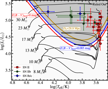
Figure 12. Hertzsprung-Russell diagram showing the region that is ruled out for a counterpart to SN 2021yja by our limits in Table 4 (red line) and assuming E(B − V)host = 0.0 mag and Dhost = 23.4 Mpc. For comparison, we show the same limits using the updated reddening value of E(B − V)host = 0.085 mag and a total-to-selective extinction ratio of RV =3.1 (blue), and the limits assuming this reddening and a farther distance of 28.8 Mpc (gold; assumed distance + 1σ). We also overplot MIST single-star evolutionary tracks for stars with initial masses 8–30 M⊙ (black lines) as well as counterparts to Type Ib, IIb, and II SNe from the literature (Cao et al. 2013; Smartt 2015; Kilpatrick et al. 2021, and references therein). For our fiducial host distance and reddening values, our limits rule out evolved massive stars >9 M⊙.
Download figure:
Standard image High-resolution imageThus while we rely on the WFPC2 image from 26 March 1997, 24.5 yr before explosion, for our best constraints on the nature of any progenitor star of SN 2021yja, we can place meaningful constraints on that star at later times when the DECam and Spitzer imaging were obtained. These limits are informative in the scenario where that star was highly variable and had a lower flux in F606W compared to its average flux (i.e., similar to variability in α Ori and the recent detection of a dimming RSG in M51 described in Levesque & Massey 2020; Jencson et al. 2022). We further explore the implications of this scenario below.
4. Discussion
4.1. CSM
Our analysis above gives rise to a somewhat confusing picture with regard to CSM around the progenitor of SN 2021yja. On one hand, we do not see some standard signs of CSM, including pronounced, narrow emission lines in early spectra, and, at first glance, the shock cooling model appears to fit our observed light curve reasonably well. On the other hand, the high UV luminosity, very blue colors, and persistent high temperature (resulting in an overly large progenitor radius from the shock cooling model), as well as the ledge-shaped feature in the early spectra, do suggest some level of early circumstellar interaction. HST UV-optical spectra from Vasylyev et al. (2022) show no sign of circumstellar interaction, but these were observed much later (7 days after explosion) than our early spectra showing the ledge. In addition, the detection of delayed radio emission (Alsaberi et al. 2021) from SN 2021yja following an initial non-detection (Ryder et al. 2021) can be taken as an indication of interaction with a non-uniform CSM, similar to the conclusion of Bostroem et al. (2019) for the SN II ASASSN-15oz. SN 2021yja was also observed in the very high-energy γ-ray domain (E > 100 GeV) by the High Energy Stereoscopic System (H.E.S.S.) Imaging Atmospheric Cherenkov Telescope Array, which will yield complementary constraints on the CSM density (H.E.S.S. Collaboration 2022, in preparation) following the work presented by Abdalla et al. (2019) and the H.E.S.S. Collaboration (2022).
One way to resolve this apparent contradiction is to infer a small amount of CSM: less than is required to produce strong emission lines, but still enough to affect the broadband light curve, especially in the UV. We turn to the literature to constrain the mass-loss rate from both directions. By modeling a sample of early SN II spectra with narrow emission lines, Boian & Groh (2020) find CSM density parameters of order D ∼ 1015−16 g cm−1, corresponding to mass loss of , where v∞ is the terminal wind speed. Our mass-loss rate must therefore be .


Dessart et al. (2017) propose a scenario in which the interaction lines are both broadened and blueshifted, which can potentially explain the ledge-shaped feature we discuss in Section 3.4. This occurs when an RSG with radius R⋆ = 501 R☉ explodes into low-density CSM (). They term this the r1w1 model. In this scenario, narrow emission lines are not seen or disappear within hours of explosion, at which time we had not yet observed the spectrum of SN 2021yja. When they add an extended atmosphere onto the RSG (r1w1h model; scale height Hρ = 0.3R⋆), the spectroscopic evolution is similar, but the light curve rises faster and is much more luminous in the UV (reaching MUVW2 ≈ − 19.5 mag). Such an extended atmosphere only requires a small energy injection during the last year before explosion (Smith & Arnett 2014; Morozova et al. 2020). Figure 13 compares the early spectra of SN 2021yja to the r1w1 and r1w1h models of Dessart et al. (2017). Notably, the extended atmosphere or r1w1h could also lead to an overestimate of the progenitor radius by a shock cooling model that was not designed to account for it. Therefore, we believe this to be the most likely scenario for the progenitor of SN 2021yja: an RSG with an extended atmosphere exploding into low-density CSM.

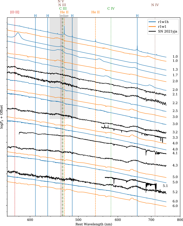
Figure 13. Comparing the early spectra of SN 2021yja to the r1w1 and r1w1h models of Dessart et al. (2017), with lines labeled as in Figure 2. These models both have low-density CSM from a mass-loss rate of order . The r1w1h model also includes an extended RSG atmosphere. Although not a perfect match to the models, the ledge-shaped feature we observe around 450–480 nm could be explained by weak circumstellar interaction, in particular by broad, blueshifted He ii and N v.

Download figure:
Standard image High-resolution image4.2. Progenitor Star
Because of our skepticism about the inferred progenitor radius (Section 4.1), the best constraints we have on the progenitor are (1) the luminosity limit from direct imaging of the field before explosion and (2) the inferred nickel mass from the light-curve tail. Unfortunately, these are also somewhat in conflict with each other: the very strict luminosity limit suggests a very low-mass progenitor (with some caveats, discussed below), whereas the very large nickel mass suggests a massive progenitor ( ≳ 20 M☉; Eldridge et al. 2019). The latter places SN 2021yja close to the upper limit for SN II progenitors (Smartt 2015; Davies & Beasor 2018, 2020a, 2020b), implying that its progenitor star ought to have MV = − 5 to −6 mag.
The limits from WFPC2 suggest that MV > − 4.4 mag, consistent with a progenitor star of initial mass < 9 M⊙ (and following the single-star models of Choi et al. 2016). We consider this a credible limit on the initial mass of the progenitor star derived using the same distance and extinction assumptions as SN 2021yja above, but we acknowledge that there is some tension with the nature of the progenitor star as inferred from the SN light curve. Our pre-explosion limit is dominated by the single epoch of WFPC2/F606W imaging from 1997, 24.5 years before explosion, which provides the deepest limits. The tension between our pre-explosion constraints on the progenitor star and those derived from SN 2021yja could be partly eased if the star were extinguished or variable on timescales of decades before core collapse.
A −0.6 to −1.4 mag discrepancy between this expectation and our derived limits could be explained by variability in the progenitor star V-band magnitude confined to a single epoch 24.5 yr prior to core collapse, similar to the variability observed in RSGs such as Betelgeuse and M51-DS1 (Levesque & Massey 2020; Jencson et al. 2022). The peak-to-peak variability in Betelgeuse was ≈1.2 mag such that even a fraction of this change in the SN 2021yja progenitor star would completely obscure a <15 M⊙ star in our WFPC2/F606W imaging. We note, however, that these are extreme cases, and evidence from RSGs observed in M31 (Soraisam et al. 2018) and M51 (Conroy et al. 2018) suggests that the vast majority of RSGs in the expected luminosity range for the SN 2021yja progenitor star do not exhibit such extreme variability. Indeed, assuming that all RSGs follow similar V- and I-band variability to that observed in M51, those observed in Conroy et al. (2018) suggest that <8% of those stars will undergo peak-to-peak dimming at MI > − 0.6 mag. However, this likelihood is highly uncertain for RSGs as a whole, and in particular, those that are <25 yr from core collapse, which may be even more variable than the overall population (e.g., Jacobson-Galán et al. 2022).
Alternatively, the CSM discussed above could significantly obscure the progenitor star in F606W if it contained a significant dust mass. Assuming Beasor et al. (2020) mass-loss rates for an RSG in this mass range ( ≈ 10−6 M☉ yr) and corresponding wind speeds (20–25 km s−1), we consider the implied effect on circumstellar extinction. Following methods in Kilpatrick et al. (2018) for a uniform wind with carbonaceous dust grains, we infer that SN 2021yja would experience a line-of-sight extinction AV ≈ 0.1 mag, in which case circumstellar extinction could not explain an anomalously low optical luminosity for the SN 2021ya progenitor star. However, we note that this is strongly dependent on the assumed mass-loss rate and wind composition, which could be significantly different.
5. Summary and Conclusions
We have presented high-cadence, early photometric and spectroscopic observations of the Type II SN 2021yja. These have conflicting interpretations with respect to the progenitor star and its CSM. On one hand, the light curve is very luminous, especially in the UV, but on the other hand, we see no narrow emission lines in the early spectra. The high luminosity on the radioactive-decay tail of the light curve also implies a large production of 56Ni (though with a large uncertainty), which suggests a large progenitor mass. However, we inspected archival HST imaging of the host galaxy of SN 2021yja and found no coincident sources that could be the progenitor. If stellar evolution models accurately describe the end state of stars, these limits suggest the progenitor was among the lowest-mass RSGs, ≲ 9 M☉.
We conclude that the most likely progenitor is an RSG with an extended envelope, and that this progenitor exploded into low-density CSM produced via a mass-loss rate of order . This CSM still has observable effects on the light curve and spectra. We emphasize that the details of the progenitor structure and CSM configuration must be considered in analyzing CCSNe; these lead to a multidimensional phase space of observables, i.e., a "zoo" of spectral features that do not map straightforwardly onto mass-loss rate or CSM density.

As we discover CCSNe increasingly early, thanks to specially designed survey strategies, detailed modeling of each well-observed event will allow us to piece together the statistics of the CCSN progenitor population. In particular, combining multiple independent lines of analysis, e.g., light-curve modeling, spectral modeling, and direct progenitor imaging, will allow us to build a complete picture of each new event, including mass-loss history, CSM density and composition, and progenitor structure. With a sample of well-studied events, we will gain a comprehensive view of the diversity of mass loss in massive stars in their final years.
We thank Luc Dessart for providing his model light curves and spectra and for insightful comments on the manuscript; Maria Jose Bustamante, Samaporn Tinyanont, César Rojas-Bravo, David Jones, and Kayla Loertscher for their effort in taking Kast data; UCSC undergraduates Cirilla Couch, Jessica Johnson, Payton Crawford, Srujan Dandu, and Zhisen Lai for their effort in taking Nickel data; Rosalie McGurk, Vivian U, and Tianmu Gao for obtaining the KCWI spectrum; and Andrew Howard and Howard Isaacson for reducing the HIRES spectrum.
Some of the data presented herein were obtained at the W. M. Keck Observatory, which is operated as a scientific partnership among the California Institute of Technology, the University of California, and the National Aeronautics and Space Administration. The Observatory was made possible by the generous financial support of the W. M. Keck Foundation. This research has made use of the Keck Observatory Archive (KOA), which is operated by the W. M. Keck Observatory and the NASA Exoplanet Science Institute (NExScI), under contract with the National Aeronautics and Space Administration. The authors wish to recognize and acknowledge the very significant cultural role and reverence that the summit of Maunakea has always had within the indigenous Hawai'ian community. We are most fortunate to have the opportunity to conduct observations from this mountain. Based on observations obtained at the international Gemini Observatory, a program of NSF's NOIRLab, which is managed by the Association of Universities for Research in Astronomy (AURA) under a cooperative agreement with the National Science Foundation. on behalf of the Gemini Observatory partnership: the National Science Foundation (United States), National Research Council (Canada), Agencia Nacional de Investigación y Desarrollo (Chile), Ministerio de Ciencia, Tecnología e Innovación (Argentina), Ministério da Ciência, Tecnologia, Inovações e Comunicações (Brazil), and Korea Astronomy and Space Science Institute (Republic of Korea). Based on observations collected at the European Organisation for Astronomical Research in the Southern Hemisphere, Chile, as part of ePESSTO+ (the advanced Public ESO Spectroscopic Survey for Transient Objects Survey). ePESSTO+ observations were obtained under ESO programs ID 1103.D-0328 and 106.216C (PI: Inserra). Based in part on observations obtained at the Southern Astrophysical Research (SOAR) telescope, which is a joint project of the Ministério da Ciência, Tecnologia e Inovações (MCTI/LNA) do Brasil, the US National Science Foundation's NOIRLab, the University of North Carolina at Chapel Hill (UNC), and Michigan State University (MSU). This publication has made use of data collected at Lulin Observatory, partly supported by MoST grant 109-2112-M-008-001. B.E.T. acknowledges parts of this research were carried out on the traditional lands of the Ngunnawal people. We pay our respects to their elders past, present, and emerging. Based in part on data acquired at the Siding Spring Observatory 2.3 m. We acknowledge the traditional owners of the land on which the SSO stands, the Gamilaraay people, and pay our respects to elders past and present. Observations using Steward Observatory facilities were obtained as part of the large observing program AZTEC: Arizona Transient Exploration and Characterization. We are grateful to the staff at Lick Observatory for their assistance with the Nickel telescope. Research at Lick Observatory is partially supported by a generous gift from Google. The SALT data reported here were taken as part of Rutgers University program 2021-1-MLT-007 (PI: Jha). This research is based on data obtained from the Astro Data Archive at NSF's NOIRLab. These data are associated with observing programs 2012B-0001 (PI J. Frieman) and 2019B-1009 (PI P. Lira). NOIRLab is managed by the Association of Universities for Research in Astronomy (AURA) under a cooperative agreement with the National Science Foundation. This research is based on observations made with the NASA/ESA Hubble Space Telescope obtained from the Space Telescope Science Institute, which is operated by the Association of Universities for Research in Astronomy, Inc., under NASA contract NAS 5-26555. These observations are associated with program GO-6359 (PI Stiavelli; Hosseinzadeh 2022). This work is based in part on observations made with the Spitzer Space Telescope, which was operated by the Jet Propulsion Laboratory, California Institute of Technology under a contract with NASA. This work makes use of observations from the Las Cumbres Observatory network.
Time domain research by the University of Arizona team and D.J.S. is supported by NSF grants AST-1821987, 1813466, 1908972, & 2108032, and by the Heising-Simons Foundation under grant #2020-1864. Research by Y.D., N.M., and S.V. is supported by NSF grants AST-1813176 and AST-2008108. J.E.A. is supported by the international Gemini Observatory, a program of NSF's NOIRLab, which is managed by the Association of Universities for Research in Astronomy (AURA) under a cooperative agreement with the National Science Foundation, on behalf of the Gemini partnership of Argentina, Brazil, Canada, Chile, the Republic of Korea, and the United States of America. K.A.B. acknowledges support from the DIRAC Institute in the Department of Astronomy at the University of Washington. The DIRAC Institute is supported through generous gifts from the Charles and Lisa Simonyi Fund for Arts and Sciences, and the Washington Research Foundation. The Las Cumbres Observatory team is supported by NSF grants AST-1911225 and AST-1911151, and NASA Swift grant 80NSSC19K1639. The UCSC team is supported in part by the Gordon and Betty Moore Foundation, the Heising-Simons Foundation, and by a fellowship from the David and Lucile Packard Foundation to R.J.F. B.E.T. and his group were supported by the Australian Research Council Centre of Excellence for All Sky Astrophysics in 3 Dimensions (ASTRO 3D), through project number CE170100013. P.J.B. is partially supported by NASA Astrophysics Data Analysis grant NNX17AF43G "Seeing Core-Collapse Supernovae in the Ultraviolet." C.A. and B.J.S. are supported by NASA grant 80NSSC19K1717 and NSF grants AST-1920392 and AST-1911074. L.G. and T.E.M.B. acknowledge financial support from the Spanish Ministerio de Ciencia e Innovación (MCIN), the Agencia Estatal de Investigación (AEI) 10.13039/501100011033 under the PID2020-115253GA-I00 HOSTFLOWS project, from Centro Superior de Investigaciones Científicas (CSIC) under the PIE project 20215AT016, and by the program Unidad de Excelencia María de Maeztu CEX2020-001058-M. L.G. also acknowledges MCIN, AEI and the European Social Fund (ESF) "Investing in your future" under the 2019 Ramón y Cajal program RYC2019-027683-I. M.G. is supported by the EU Horizon 2020 research and innovation program under grant agreement No. 101004719. M.N. is supported by the European Research Council (ERC) under the European Union's Horizon 2020 research and innovation program (grant agreement No. 948381) and by a Fellowship from the Alan Turing Institute.
Facilities: ADS - , ARC (DIS) - Astrophysical Research Consortium 3.5m Telescope at Apache Point Observatory, ATT (WiFeS) - Advanced Technology Telescope, Blanco (DECam) - , Bok (B&C) - , CTIO:PROMPT - , FLWO:1.2 m (KeplerCam) - , FTN (FLOYDS - , MuSCAT3) - , FTS (FLOYDS) - , Gemini:South (GSAOI) - , HST (WFPC2) - , Keck:I (HIRES) - , Keck:II (KCWI - , NIRES) - , LCOGT (Sinistro) - , LO:1 m (Lulin Compact Imager) - , Meckering:PROMPT - , MMT (Binospec - , MMIRS) - , NED - , Nickel (Direct Imaging Camera) - , NTT (EFOSC - , SOFI) - , OSC - , SALT (RSS) - , Shane (Kast) - , SOAR (Goodman - , TripleSpec) - , Spitzer (IRAC) - , Swift (UVOT) - , Thacher -
Software: Astropy (Astropy Collaboration et al. 2018), BANZAI (McCully et al. 2018), Binospec Pipeline (Kansky et al. 2019), corner (Foreman-Mackey 2016), DoPHOT (Schechter et al. 1993), emcee (Foreman-Mackey et al. 2013), FLOYDS pipeline (Valenti et al. 2014), hst123 (Kilpatrick et al. 2021), IPython (Perez & Granger 2007), IRAF (National Optical Astronomy Observatories 1999), lcogtsnpipe (Valenti et al. 2016), Light Curve Fitting (Hosseinzadeh & Gomez 2020), KCWI Data Reduction Pipeline (Rizzi et al. 2021), Matplotlib (Hunter 2007), MMIRS Pipeline (Chilingarian et al. 2013), NumPy (Oliphant 2006), photpipe (Rest et al. 2005), POTPyRI (K. Paterson et al. 2022, in preparation), PyKOSMOS (Davenport 2021), PyRAF (Science Software Branch at STScI 2012), PySALT (Crawford et al. 2010), PyWiFeS (Childress et al. 2014), QFitsView (Ott 2012), SciPy (Virtanen et al. 2020), Spextool (Cushing et al. 2004), xtellcor (Vacca et al. 2003).
Appendix A: Photometry Reduction
Las Cumbres Observatory images are preprocessed by BANZAI (McCully et al. 2018). We extracted aperture photometry from images taken under the Global Supernova Project using lcogtsnpipe, which is based on PyRAF (Science Software Branch at STScI 2012). We calibrated UBV magnitudes to images of Landolt (1992) standard fields (Vega magnitudes) taken on the same night with the same telescope, and we calibrated gri magnitudes to the Pan-STARRS1 (PS1) 3πSurvey (AB magnitudes; Chambers et al. 2016).
Las Cumbres images (including MuSCAT3) taken under the Young Supernova Experiment, as well as data from the Lulin 1 m telescope and Nickel 1 m telescope, were reduced using photpipe (Rest et al. 2005). griz magnitudes were calibrated to PS1 3π, and u magnitudes were calibrated to SkyMapper (Onken et al. 2019).
Thacher data were calibrated with nightly dark and bias frames and master flat-field frames in each band. We used DoPHOT (Schechter et al. 1993) to perform PSF modeling and to obtain the counts in SN 2021yja as well as 12 reference stars in the Pan-STARRS1 catalog with r-band magnitudes between 13.7 and 16.6 mags. Preliminary magnitudes were calculated for SN 2021yja using zero-points derived for each image based on the reference star fluxes. Then a second pass was made on the data to perform a first order color correction to account for the bandpass mismatches between the Thacher and Pan-STARRS1 filters.
Unfiltered DLT40 light curves consist of aperture photometry calibrated to r-band catalogs from the AAVSO Photometry All-Sky Survey (APASS; Henden et al. 2009).
Swift data were analyzed using an updated version of the pipeline for the SOUSA (Brown et al. 2014). Zero-points from Breeveld et al. (2011) were used with time-dependent sensitivity corrections updated in 2020 and an aperture correction calculated for 2021.
We perform image subtraction on each KeplerCam image with HOTPANTS (Becker 2015), using archival PS1 3πimages as reference templates. Instrumental magnitudes were measured using PSF fitting and calibrated to PS1 3π.
MMIRS imaging data were reduced using a custom pipeline (adapted from POTPyRI; K. Paterson et al. 2022, in preparation) that performs standard dark-current subtraction, flat-fielding, sky background estimation and subtraction, astrometric alignments, and final stacking of the individual exposures. The images were photometrically calibrated with aperture photometry of relatively isolated stars in the MMIRS images with cataloged JHKs-band magnitudes in the Two Micron All Sky Survey (2MASS; Skrutskie et al. 2006). We then performed aperture photometry on SN 2021yja. The measurement uncertainities are dominated by scatter in the zero-point estimation from the 2MASS stars.
Appendix B: Spectroscopy Reduction
The optical and near-infrared spectra of SN 2021yja are logged in Table 5. These will be made available on the Weizmann Interactive Supernova Data Repository (Yaron & Gal-Yam 2012) after publication.
Table 5. Log of Spectroscopic Observations
| MJD | Telescope | Instrument | Phase | Exposure | Wavelength | Resolution |
|---|---|---|---|---|---|---|
| (d) | Time (s) | Range (nm) | λ/Δλ | |||
| 59466.507 | FTN | FLOYDS | 2.1 | 600 | 335–930 | 380 |
| 59466.596 | FTS | FLOYDS | 2.2 | 600 | 335–930 | 250 |
| 59467.643 | FTS | FLOYDS | 3.2 | 900 | 335–930 | 250 |
| 59467.680 | SSO 2.3 m | WiFeS | 3.3 | 3600 | 559–850 | 3000 |
| 59468.484 | MMT | Binospec | 4.1 | 1440 | 383–920 | 650 |
| 59468.769 | FTS | FLOYDS | 4.3 | 900 | 335–930 | 250 |
| 59469.480 | MMT | Binospec | 5.1 | 1440 | 569–721 | 2900 |
| 59469.606 | FTS | FLOYDS | 5.2 | 900 | 335–930 | 250 |
| 59471.312 | NTT | EFOSC | 6.9 | 900 | 338–932 | 350 |
| 59471.590 | FTS | FLOYDS | 7.1 | 900 | 335–930 | 250 |
| 59471.652 | Keck II | KCWI | 7.2 | 60 | 350–560 | 1250 |
| 59472.653 | FTS | FLOYDS | 8.2 | 1500 | 335–930 | 250 |
| 59474.485 | Keck II | NIRES | 10.0 | 1200 | 965–2460 | 2700 |
| 59474.549 | FTN | FLOYDS | 10.1 | 900 | 335–930 | 380 |
| 59475.734 | FTS | FLOYDS | 11.3 | 900 | 335–930 | 250 |
| 59476.975 | SALT | RSS | 12.5 | 1495 | 350–930 | 1000 |
| 59477.461 | MMT | MMIRS | 13.0 | 1200 | 940–1510 | 960 |
| 59477.542 | FTN | FLOYDS | 13.1 | 900 | 335–930 | 380 |
| 59478.484 | FTN | FLOYDS | 14.0 | 600 | 335–930 | 460 |
| 59479.552 | FTN | FLOYDS | 15.1 | 900 | 335–930 | 380 |
| 59479.969 | SALT | RSS | 15.5 | 1495 | 350–930 | 1000 |
| 59480.641 | FTS | FLOYDS | 16.1 | 600 | 335–930 | 270 |
| 59481.332 | NTT | EFOSC | 16.8 | 900 | 338–932 | 350 |
| 59481.961 | SALT | RSS | 17.5 | 1495 | 350–930 | 1000 |
| 59482.276 | NTT | SOFI | 17.8 | 960 | 950–2520 | 600 |
| 59482.515 | FTN | FLOYDS | 18.0 | 900 | 335–930 | 380 |
| 59483.490 | Shane | Kast | 19.0 | 630/600 | 300–1050 | 600 |
| 59483.557 | FTN | FLOYDS | 19.0 | 600 | 335–930 | 460 |
| 59486.549 | FTN | FLOYDS | 22.0 | 600 | 335–930 | 460 |
| 59487.519 | FTN | FLOYDS | 23.0 | 900 | 335–930 | 380 |
| 59488.550 | FTN | FLOYDS | 24.0 | 600 | 335–930 | 460 |
| 59490.474 | FTN | FLOYDS | 25.9 | 900 | 335–930 | 380 |
| 59490.721 | FTS | FLOYDS | 26.2 | 600 | 335–930 | 270 |
| 59492.641 | FTS | FLOYDS | 28.1 | 2400 | 335–930 | 250 |
| 59493.371 | Bok | B&C | 28.8 | 1000 | 601–716 | 3400 |
| 59494.301 | Bok | B&C | 29.7 | 1000 | 340–759 | 700 |
| 59494.634 | FTS | FLOYDS | 30.1 | 600 | 335–930 | 270 |
| 59495.760 | FTS | FLOYDS | 31.2 | 900 | 335–930 | 250 |
| 59496.726 | FTS | FLOYDS | 32.1 | 600 | 335–930 | 270 |
| 59498.522 | FTN | FLOYDS | 33.9 | 1500 | 335–930 | 380 |
| 59501.566 | FTN | FLOYDS | 37.0 | 900 | 335–930 | 380 |
| 59504.475 | FTS | FLOYDS | 39.8 | 600 | 335–930 | 270 |
| 59508.544 | FTN | FLOYDS | 43.9 | 900 | 335–930 | 380 |
| 59509.457 | Keck I | HIRES | 44.8 | 3001 | 364–799 | 50,000 |
| 59516.578 | FTS | FLOYDS | 51.9 | 600 | 335–930 | 270 |
| 59516.668 | SSO 2.3 m | WiFeS | 52.0 | 3600 | 350–900 | 3000 |
| 59517.522 | FTS | FLOYDS | 52.8 | 900 | 335–930 | 250 |
| 59517.598 | SSO 2.3 m | WiFeS | 52.9 | 3600 | 350–900 | 3000 |
| 59519.524 | FTN | FLOYDS | 54.8 | 600 | 335–930 | 460 |
| 59524.458 | FTN | FLOYDS | 59.7 | 900 | 335–930 | 380 |
| 59526.339 | Shane | Kast | 61.6 | 1703/1698 | 300–1050 | 600 |
| 59533.355 | Shane | Kast | 68.6 | 630/600 | 300–1050 | 600 |
| 59533.719 | FTS | FLOYDS | 68.9 | 900 | 335–930 | 250 |
| 59543.294 | Shane | Kast | 78.4 | 630/600 | 300–1050 | 600 |
| 59551.642 | FTS | FLOYDS | 86.7 | 900 | 335–930 | 250 |
| 59560.422 | FTS | FLOYDS | 95.5 | 900 | 335–930 | 250 |
| 59565.133 | SOAR | TripleSpec | 100.2 | 960 | 940–2460 | 3500 |
| 59565.273 | MMT | MMIRS | 100.3 | 1440 | 940–1510 | 960 |
| 59566.051 | SOAR | Goodman | 101.1 | 600 | 300–705 | 850 |
| 59566.237 | MMT | MMIRS | 101.3 | 1440 | 940–1510 | 960 |
| 59571.537 | FTS | FLOYDS | 106.5 | 900 | 335–930 | 250 |
| 59580.564 | FTS | FLOYDS | 115.5 | 900 | 335–930 | 250 |
| 59582.461 | FTS | FLOYDS | 117.4 | 1000 | 335–930 | 250 |
| 59586.100 | Shane | Kast | 121.0 | 630/600 | 300–1050 | 600 |
| 59593.488 | FTS | FLOYDS | 128.4 | 1000 | 335–930 | 250 |
| 59605.103 | Shane | Kast | 139.9 | 1230/1200 | 300–1050 | 600 |
| 59605.144 | ARC 3.5 m | DIS | 139.9 | 1800 | 380–950 | 1000 |
| 59611.128 | Shane | Kast | 145.9 | 930/900 | 300–1050 | 600 |
Note. Wavelength range and resolution are approximate. Exposure times for Kast spectra are for the blue and red halves, respectively.
FLOYDS spectra were reduced using the FLOYDS pipeline (Valenti et al. 2014), which is based on PyRAF.
The Kast and Goodman spectra were reduced using standard IRAF/PyRAF and Python routines for bias/overscan subtractions and flat-fielding. The wavelength solution was derived using arc lamps while the final flux calibration and telluric lines removal were performed using spectrophotometric standard star spectra.
The EFOSC2 and SOFI spectra were reduced using the PESSTO pipeline (Smartt et al. 2015).
Basic 2D reductions for the MMIRS standard long-slit zJ single-order spectra were performed using the MMIRS data reduction pipeline (Chilingarian et al. 2013), including flat-fielding, subtraction of AB pairs to remove the sky background, and wavelength calibrations. We then performed 1D spectral extractions using standard tasks in IRAF. Flux calibrations and corrections for the strong near-infrared telluric absorption features were performed using observations of the A0V standards HD 13165, HIP 25347, and HIP 25117 taken immediately preceding each of the observations of the SN. We used the method of Vacca et al. (2003) implemented with the IDL tool XTELLCOR_GENERAL developed by Cushing et al. (2004) as part of the Spextool package.
The SALT data were reduced using a custom pipeline based on the PySALT package (Crawford et al. 2010).
Each WiFeS observation was reduced using PyWiFeS (Childress et al. 2014) producing a 3D cube file for each grating that has had bad pixels and cosmic rays removed, while we combined our two 1800 exposures that we took on the night. We extracted spectra from the calibrated 3D data cube using QFitsView (Ott 2012) using an aperture similar to the seeing on the night (average seeing of 1.1 − 1.6'' on the night). For background subtraction, we extract a part of the sky that is isolated from the source using a similarly sized aperture.
Binospec data were reduced using the Binospec pipeline (Kansky et al. 2019). While an internal flux calibration into relative flux units from throughput measurements of spectrophotometric standard stars is provided in the pipeline, we obtained our own spectrophotometric standard observations throughout the semester and created our own sensitivty function for flux calibration.
Reductions of Bok B&C spectra were carried out using IRAF including bias subtraction, flat fielding, and optimal extraction of the spectra. Flux calibration was achieved using spectrophotometric standards observed at an air mass similar to that of each science frame, and the resulting spectra were median combined into a single 1D spectrum for each epoch.
The DIS spectrum was reduced using PyKOSMOS (Davenport 2021) using standard techniques for bias/overscan subtraction, flat-field correction, 1D extraction, and wavelength calibration. Flux calibration was performed using the optical flux standard star LTT2415. 1D observations were cleaned and median combined to produce the final spectrum.
The HIRES spectra were reduced using the standard procedure of the California Planet Search (Howard et al. 2010). We extracted the two orders of interest, containing the DIB and the Na i D lines. For each order, we median-combined the four exposures, masked the lines of interest, and then modeled the continuum by smoothing with a second-order Savitzky & Golay (1964) filter with a width of 555 pixels. Figure 5 shows this spectrum divided by the continuum.
The KCWI spectra were reduced following the standard procedures used in the python version of the KCWI Data Reduction Pipeline (Rizzi et al. 2021). The spectra were extracted from the data cube using QFitsView (Ott 2012).
The NIRES spectrum was reduced following standard procedures described in the IDL package Spextool version 5.0.2 for NIRES (Cushing et al. 2004). The extracted 1D spectrum was flux calibrated and also corrected for telluric features with xtellcorr version 5.0.2 for NIRES (Vacca et al. 2003) making use of observations of an A0V standard star.
We used the Spextool IDL package (Cushing et al. 2004) to reduce the TripleSpec data, and we subtracted consecutive AB pairs to remove the sky and the dark current. The pixel-to-pixel gain variations in the science frames were corrected by dividing for the normalized master flat. We calibrated 2D science frames in wavelength by using CuHeAr Hollow Cathode comparison lamps. To correct for telluric features and to flux-calibrate the SN spectra, we observed the HIP 19001 A0V telluric standard after the SN and at a similar air mass. After the extraction of the individual spectra from the 2D frames, we used the xtellcorr task (Vacca et al. 2003) included in the Spextool IDL package to perform the telluric correction and the flux calibration.
Footnotes
- 47
Throughout this work, we use "SNe II" to refer to Type IIP and Type IIL SNe (Barbon et al. 1979), but not Type IIb or Type IIn SNe.
- 48
NGC 1325 previously hosted SN 1975S, which was not spectroscopically classified (Wegner 1977).
- 49
After a final reduction of these images, we report updated magnitudes in Figure 1 and its associated online-only table.
- 50
Sinistro data were obtained under both the GSP and the YSE programs.