


Abstract
Continuous wavelet analysis has been increasingly employed in various fields of science and engineering due to its remarkable ability to maintain optimal resolution in both space and scale. Here, we introduce wavelet-based statistics, including the wavelet power spectrum, wavelet cross correlation, and wavelet bicoherence, to analyze the large-scale clustering of matter. For this purpose, we perform wavelet transforms on the density distribution obtained from the one-dimensional Zel'dovich approximation and then measure the wavelet power spectra and wavelet bicoherences of this density distribution. Our results suggest that the wavelet power spectrum and wavelet bicoherence can identify the effects of local environments on the clustering at different scales. Moreover, we apply the statistics based on the three-dimensional isotropic wavelet to the IllustrisTNG simulation at z = 0, and investigate the environmental dependence of the matter clustering. We find that the clustering strength of the total matter increases with increasing local density except on the largest scales. Besides, we notice that the gas traces dark matter better than stars on large scales in all environments. On small scales, the cross correlation between the dark matter and gas first decreases and then increases with increasing density. This is related to the impacts of the active galactic nucleus feedback on the matter distribution, which also varies with the density environment in a similar trend to the cross correlation between dark matter and gas. Our findings are qualitatively consistent with previous studies on matter clustering.
Export citation and abstract BibTeX RIS

Original content from this work may be used under the terms of the Creative Commons Attribution 4.0 licence. Any further distribution of this work must maintain attribution to the author(s) and the title of the work, journal citation and DOI.
1. Introduction
The standard cosmological model (Lambda cold dark matter) states that the hierarchical matter clustering evolved from the random primordial fluctuations via gravitational instability, as revealed by the observed pattern of spatial distribution for luminous objects (Tegmark et al. 2004). However, luminous objects are made up of baryons, whose clustering is not completely consistent with that of the dark matter (DM) component because of a series of physical processes such as radiative cooling, star formation, and feedback processes. With hybrid N-body/hydrodynamic simulations, the baryonic effects on the large-scale clustering of matter have been extensively studied in Fourier space, and these studies show that the deviation between baryons and DM in mass distribution depends on the scale and redshift (e.g., Chisari et al. 2019; van Daalen et al. 2020; Yang et al. 2020). Moreover, many studies indicate that the clustering of both DM and baryonic matter is environmentally dependent (e.g., Abbas & Sheth 2005; Peng et al. 2010; Wang et al. 2018; Man et al. 2019). However, usual statistical schemes based on the ordinary Fourier transform, e.g., power spectrum and bispectrum, cannot be used to measure the environmental and scale dependence of the matter clustering at the same time, since these schemes do not contain any positional information on the signal. A straightforward solution to overcome this problem is to use the technique of the windowed Fourier transform (WFT), which takes harmonic waves multiplied by a window of fixed width as basis functions, hence enabling us to gain the positional and scale information simultaneously (Gabor 1946).
However, the fixed window size of the WFT leads to a poor space-scale resolution (e.g., Kaiser & Hudgins 1994; Romeo et al. 2004; Gao & Yan 2011). If we set the window size to be small enough, then the spatial resolution certainly matches the signal, but the scale/frequency localization is too poor to resolve the large scales/low frequencies. If we choose a wider window in order to have a finer scale/frequency resolution, the spatial resolution becomes too coarse to detect small-scale structures. Therefore, the WFT is not a suitable tool for analyzing signals with a wide range of scales, such as spatial distributions of the DM and galaxies.
An alternative way to achieve simultaneous analysis of space and scale is the wavelet transform (WT), which provides an adaptive space-scale resolution (e.g., Daubechies 1992; Kaiser & Hudgins 1994; Chui 1997; Torrence & Compo 1998; Van den Berg 2004; Mallat 2009; Addison 2017). WT analysis decomposes a signal into separate scale components using a set of scaled and shifted wavelets, which are well localized in both real and Fourier space. Consequently, the local features of the signal at different scales are revealed by this decomposition. WT methods can be classified into the discrete wavelet transform (DWT) and the continuous wavelet transform (CWT). The DWT, using orthogonal wavelet bases, operates over scales and positions based on the integer power of 2, hence giving the most compact representation of the signal. This leads to the effectiveness and ease of implementation of the DWT, which hence is particularly useful for information on compression (e.g., Khalifa et al. 2008; Abdulazeez et al. 2020). Due to its advantages, the DWT has also been applied to study the large-scale structure of the universe (e.g., Fujiwara & Soda 1996; Pando & Fang 1996; Pando et al. 1998, 2004; Fang & Feng 2000; Romeo et al. 2004; Liu & Fang 2008; Lu et al. 2010). However, there are mainly two drawbacks in the DWT caused by dyadic scales. First, the DWT provides a poor scale resolution so that some meaningful features of a signal cannot be detected. Second, it lacks translational invariance. The so-called translational invariance means that if a signal is translated, then its wavelet coefficients are translated by the same amount without other modifications at every scale (Addison 2017). Obviously, this is not the case for the DWT. A small translation of the signal can make the discrete wavelet coefficients vary substantially on different scales, thereby the total energy in the wavelet domain is not conserved after the signal was shifted. These drawbacks suggest that the DWT is not suitable for analyzing signals with extremely high complexity.
In contrast to the DWT, the CWT allows the scale and translation parameters to continuously change, which makes it translationally invariant and redundant. The redundancy guarantees that the CWT can provide high-resolution results, which are much easier to interpret than those obtained with the DWT (Aguiar-Conraria & Soares 2014; Addison 2018). As a result, the CWT is becoming more and more popular across different disciplines, including geophysics, biomedicine, economics, astrophysics, fluid mechanics, and so on. For instance in astrophysics and cosmology, the CWT is used for the detection of 21 cm signals (e.g., Gu et al. 2013), the detection of baryonic acoustic oscillations (e.g., Tian et al. 2011; Arnalte-Mur et al. 2012; Labatie et al. 2012), the detection of substructures in two-dimensional (2D) mass maps (e.g., Flin & Krywult 2006; Schwinn et al. 2018), the analysis of turbulence evolution in the intracluster medium (e.g., Shi et al. 2018; Roh et al. 2019), the correlation analysis of galactic images (e.g., Frick et al. 2001; Tabatabaei et al. 2013), the analysis of the multifractal character of the galaxy distribution (e.g., Martínez et al. 1993; Rozgacheva et al. 2012), and the analysis of cosmic microwave background maps (e.g., Cayón et al. 2001; Starck et al. 2004; González-Nuevo et al. 2006; Curto et al. 2011).
The main problem faced by the CWT, e.g., when analyzing one-dimensional (1D) signals, is that its classical inverse formula is a double integration, which results in a heavy computational effort in recovering the original signal. Although there is an alternative inverse transform formula in the form of a single integral for the complex-valued wavelets, the real wavelets have generally been considered to have no such simple inverse transformation (Delprat et al. 1992; Aguiar-Conraria & Soares 2014). In our previous work (Wang & He 2021), we proposed a novel scheme of constructing continuous wavelets to overcome this problem, in which the wavelet functions are obtained by taking the first derivative of smoothing functions with regard to the positively defined scale parameter. With this scheme, the original signal is recovered easily by integrating the wavelet coefficients with respect to the scale parameter. As an inspired example, we took the Gaussian function as a smoothing function to derive the wavelet dubbed the Gaussian-derived wavelet (hereafter GDW) and briefly discussed its preliminary application to the matter power spectrum, demonstrating the success of this scheme.
In this work, we use local statistics established on wavelet coefficients to further investigate the potential of the GDW for analyzing the large-scale clustering of matter. Specifically, the wavelet power spectrum (WPS), the wavelet cross correlation (WCC), and the wavelet bicoherence (WBC) are employed here. The WPS and WCC were first introduced by Hudgins et al. (1993) to examine atmospheric turbulence. The WPS measures the variance of a signal at various scales within some local region, and the WCC is used to quantify similarities between two signals. The WBC was originally proposed by van Milligen et al. (1995a, 1995b) to detect the short-lived structures induced by phase coupling in turbulence. Moreover, the cosmic baryonic density distribution at late times is similar to a fully developed turbulence (Shandarin & Zel'dovich 1989; He et al. 2006), which enlightens us to apply these tools to the context of the structure formation of the universe. To illustrate our approach in a more intuitive way, we shall use the 1D matter distributions, since a great deal of work on the large-scale structure of the universe is accomplished using 1D cosmology models (Gouda & Nakamura 1989; Fujiwara & Soda 1996; Tatekawa & Maeda 2001; Miller & Rouet 2010; Manfredi et al. 2016). The Zel'dovich approximation is a simple model that provides a good approximated solution for the nonlinear evolution of collisionless matter (Zel'dovich1970). In the 1D case, the Zel'dovich approximation is proved to be an exact solution in the fully nonlinear regime until the first singularity appears (Soda & Suto 1992). It is straightforward and efficient to calculate the 1D Zel'dovich solution, and so we discuss our analysis method with it. First, we decompose the density fields obtained from the 1D Zel'dovich approximation into wavelet components at different positions and scales. Then, by measuring the WPS and WBC of matter densities based on these components, we investigate the effects of the density environment on the matter clustering.
To further demonstrate the ability of wavelet statistics in characterizing the environmental dependence of the matter clustering, we generalize them to the three-dimensional (3D) versions and then apply them to the 3D density fields for the different matter components in the IllustrisTNG simulation (Springel et al. 2018; Naiman et al. 2018; Nelson et al. 2018; Pillepich et al. 2018; Marinacci et al. 2018). By measuring the WPS and WCC, we can investigate (1) the variation of the clustering strength with the density environment at given scales, (2) the variation of the cross correlations between different matter components with the density environment at given scales, and (3) the baryonic effects on the matter clustering in different density environments.
This paper is organized as follows. In Section 2, we describe the characteristics of the GDW, the theory of the CWT, and wavelet-based statistical tools. In Section 3, we briefly introduce the data we used, including 1D Zel'dovich approximation and density fields in IllustrisTNG. In Section 4, we give the numerical results for the matter clustering. Finally, in Section 5, we discuss and summarize our results.
2. Methods of Continuous Wavelet Analysis
In this section, we briefly review the definition of the CWT based on the GDW in 1D and then introduce the wavelet-based statistical tools, i.e., the WPS, the WCC function, and the WBC. To assess their significance, statistical errors are then discussed. Finally, we give the correspondence between the wavelet scale and the Fourier wavenumber for the GDW. The 3D isotropic CWT and the statistics formulated on it are given in Appendix B.
2.1. GDW and CWT
The GDW used in this work is defined as the first derivative of the Gaussian smoothing function with respect to the scale parameter w, multiplied by a factor  ,
,

where  denotes the Gaussian smoothing function with the scale parameter w greater than zero. The prefactor
  on the right-hand side of Equation (1) ensures that the energy of the wavelet is unaffected by the scale parameter.
3
The Fourier transform of the GDW is given by
on the right-hand side of Equation (1) ensures that the energy of the wavelet is unaffected by the scale parameter.
3
The Fourier transform of the GDW is given by
through which the scale parameter w is defined as the peak wavenumber of  , i.e., the wavenumber at which
  takes the maximum value, as demonstrated in Figure 1. It can be seen from Equations (1) and (2) that the GDW satisfies the conditions of admissibility, similarity, and regularity. In fact, the GDW is the same as the Mexican hat wavelet in 1D, except for their constant factors. This is illustrated by substituting
  into Equation (1), where a is the scale parameter for the traditional CWT.
4
However, as pointed out by Wang & He (2021), the 3D GDW is an anisotropic separable wavelet function, which is not a 3D Mexican hat wavelet. At present, we are only concerned with the 1D case.
into Equation (1), where a is the scale parameter for the traditional CWT.
4
However, as pointed out by Wang & He (2021), the 3D GDW is an anisotropic separable wavelet function, which is not a 3D Mexican hat wavelet. At present, we are only concerned with the 1D case.
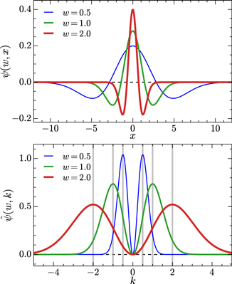
Figure 1. The GDW, ψ(w, x) (top) and the corresponding Fourier transform  (bottom) for three scale parameters, w = 0.5, 1.0, and 2.0. The gray vertical lines denote wavenumbers where
  takes the maximum.
Download figure:
Standard image High-resolution imageThe wavelet function ψ(w, x) is then used to perform the WT of a 1D signal f(x) as follows:

Note that there is no complex conjugate in Equation (3) since both signal and wavelet are real. The WT, Equation (3), is nothing but a convolution of the signal with wavelets at different scales, which can be implemented efficiently by the fast Fourier transform (FFT) technique. As a function of scale w and space x, from the WT we can clearly see how different scale features are localized in space. However, it is not possible to achieve arbitrarily good resolution in space and scale simultaneously (Chui 1997; Addison 2017). As illustrated in Figure 1, a narrower (wider) wavelet provides better (poorer) spatial resolution accompanied by poorer (better) frequency resolution. This fact is quantified in terms of the uncertainty principle ΔxΔk ≳ 1/2 for the GDW, where Δx is the standard deviation of the wavelet in real space and Δk is the standard deviation in frequency (Chui 1997).
The greatest convenience brought to us by the definition of GDW is that the signal can be reconstructed through a single integral of the wavelet coefficients. Combining Equations (1) and (3), we have

where fs(w, x) refers to the smoothed field under the scale w and is given by

By integrating Equation (4) with respect to w, we get the single-integral inverse transform as shown below,

where the integral constant C is equal to fs(w = 0, x), and generally C = 0 for, say, the density contrast field of the universe. Compared with the usual reconstruction formula for the CWT found in most wavelet literature, e.g., Addison (2017), our reconstruction formula defined by Equation (6) is much easier to compute numerically and generalize to integrations of higher dimensions.
2.2. Parseval's Theorem for the CWT
Parseval's theorem is an important result in Fourier transform, which states that the inner product between signals is preserved in going from time to the frequency domain. Similarly, there is an analog of Parseval's theorem for the WT (Hudgins et al. 1993), the form of which is expressed as

where Wf
(w, x) and Wg
(w, x) are WTs for f(x) and g(x), respectively,  is the admissibility constant, and equals 1/2 for the GDW. If f and g are the same, then we have

2.3. WPS and WCC
We assume that the signal f(x) satisfies the periodic boundary condition with period Lb, which is a usual choice for studying a typical region of the universe. Then for a subregion of the signal L ≤ Lb, the local WPS is defined as

We can see that Equation (9) refers to the variance at the scale w within the spatial region L, since ∣Wf (w, x)∣2 is just the variance per area at the space-scale plane, as referred to by the Parseval's theorem, Equation (8). According to the Fourier Parseval's theorem for periodical signals, we can obtain the relationship between the global wavelet and Fourier power spectrum, which is given by
where  is the Fourier transform of Wf
(w, x),
is the Fourier transform of Wf
(w, x),  is the Fourier power spectrum of the signal, and
  denotes the Fourier power spectrum of the wavelet. Obviously, the global WPS of a signal is the average of its Fourier power spectrum weighted by the Fourier power spectrum of the corresponding wavelet function over all wavenumbers.
Then given two signals f(x) and g(x) with WTs Wf (w, x) and Wg (w, x), we can define the cross-wavelet transform (XWT) as

i.e., it measures the local covariance at each spatial position and scale, as revealed by Equation (7). By integrating the XWT over a finite spatial region, we get the normalized local WCC as follows:
which can take on values between −1 (perfect anticorrelation) and 1 (perfect correlation).
2.4. WBC and Error Estimation
The main content of this subsection is based on van Milligen et al. (1995a, 1995b), and we refer the interested readers to these two references for the details.
The Fourier bispectrum is the lowest order statistic that measures the amount of phase coupling of harmonic modes within a signal. By analogy, the WBS is given as
where w1 + w2 = w (frequency sum rule). The WBS measures the nonlinear interplay within the local region L between scale components w1, w2, and w such that the sum rule is satisfied. In the case of completely random phases of the signal,  is statistically zero. However, once a coherent structure is formed by the phase coupling,
  will take significant nonzero values. The WBS usually is normalized in the following way:
which is called the WBC, attaining values between 0 and 1. Throughout this paper we will use it to measure the nonlinear behaviors of matter clustering instead of the WBS. In addition, it is convenient to introduce the summed WBC defined as
where the summation is taken over all w1 and w2 such that w1 + w2 equals w and s(w) is the number of summands in the summation. In addition, as a measure of the total nonlinearity in the chosen region of the signal, the total WBC is defined by averaging the squared WBC over all points in the scale-scale plane as

where S is the total number of points (w1, w2) in the scale-scale plane.
In practice for discrete sampled signals, integrations over the interval L involved in calculating the statistics mentioned above are carried out with summation over N sample points. By the law of large numbers, an integration over L suffers a relative statistical error of  . In addition, the fact that CWTs are non-orthogonal leads to the wavelet coefficients not all being statistically independent (van Milligen et al. 1995a, 1995b, 1997). If continuous wavelets ψ(x) and ψ*(x + d0) satisfy ∫ψ(x)ψ*(x +d0)dx = 0, then they can be regarded as approximately orthogonal and the corresponding wavelet coefficients are statistically independent. In the case of the GDW, independent wavelet coefficients are separated by distance d0/w at each scale, where
  . Then the number of statistical independent points on the interval L is
  , where ksamp = 2π/Δx is the sampling frequency. Thus for the WPS, its statistical error is estimated by
By applying similar estimates for all integral terms in Equation (12) and according to error propagation, we obtain the statistical noise level for the WCC,
Equation (18) is called the statistical noise level because it is the cross-correlation value that can be achieved by Gaussian noise and is caused by using a limited number of values in the integration. Notice that this noise level is scale dependent, suggesting that the interpretation of the signal becomes increasingly significant as the scale decreases. Just like the approach above, we can obtain the noise level of the WBC as shown below,
2.5. Relationship between Scale and Wavenumber
To facilitate the comparison between wavelet and Fourier spectra, we need to ascertain the relationship between the scale parameter w and the equivalent Fourier wavenumber. Meyers et al. (1993) and Torrence & Compo (1998) suggest that the relationship between them can be derived analytically for a particular wavelet function by performing a WT of a cosine wave with a known period, such as  , and then computing the scale w at which the scalogram reaches its maximum. Following their method, the scalogram of
  is first computed with the GDW, and the result is
which is depicted in Figure 2. The scale parameter that makes  take the maximum value should be equivalent to the wavenumber kF
, since the Fourier power spectrum of a cosine wave is an impulse at kF
. Therefore, by solving
take the maximum value should be equivalent to the wavenumber kF
, since the Fourier power spectrum of a cosine wave is an impulse at kF
. Therefore, by solving  , we get the correspondence between the wavelet scale and Fourier wavenumber,

The relation of Equation (21) shows that the wavelet scale is proportional to the Fourier wavenumber. 5 In the next sections, we will present our results in terms of the equivalent Fourier wavenumber kF instead of w, and we drop the subscript "F" for simplicity of notation.
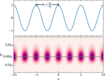
Figure 2. The squared WT plot of a cosine function. Upper panel: a cosine wave of period λ = 2π/kF
. Lower panel: the corresponding contour plot of  for the cosine wave. The gray horizontal line indicates that
  reaches its maximum value at w ≈ 0.89kF
.
reaches its maximum value at w ≈ 0.89kF
.
Download figure:
Standard image High-resolution imageFor the convenience of the readers, in Table 1, we list all the notations used in our paper, with their meanings and corresponding acronyms.
Table 1. Notations Used in This Paper with Their Meanings and Acronyms a
| Notation | Meaning | Acronym |
|---|---|---|
| ψ(w, x) | Gaussian-derived wavelet | GDW |

| Fourier transform of the GDW | |
| Wf (w, x) | Wavelet transform | WT |

| Fourier transform of the WT | |

| Wavelet power spectrum | WPS |

| Fourier power spectrum | |
| XWTf−g (w, x) | Cross-wavelet transform | XWT |

| Wavelet cross correlation | WCC |

| Wavelet bispectrum | WBS |

| Wavelet bicoherence | WBC |

| Summed WBC | |

| Total WBC |
Note.
a In this table, we only list the symbols associated with the 1D CWT. The same notation convention is also used for the quantities based on the 3D isotropic CWT, except that the scalars x and k are replaced with vectors r and k, and the length L is replaced with volume V.Download table as: ASCIITypeset image
3. Data Sets
In this work, we use two types of data, i.e., the 1D density fields obtained from a Zel'dovich approximation and the 3D density fields of the IllustrisTNG simulations. In the 1D case, the Zel'dovich approximation provides the exact nonlinear solution for the perturbative equations of collisionless matter up to the first appearance of orbit-crossing singularities (Soda & Suto 1992). Due to easy implementation and fast computation of the 1D Zel'dovich exact solution, we will demonstrate the usefulness of our method with it before further analyzing the cosmological simulation IllustrisTNG.
3.1. Zel'dovich Approximation in One Dimension
The fundamental idea of the Zel'dovich approximation is the transformation between Eulerian and Lagrangian coordinates, i.e.,

where x and q are the Eulerian and Lagrangian coordinates, respectively. Then by applying the mass conservation to Equation (22), the density contrast is given explicitly by

where  with η = q/Lb
being the dimensionless coordinates divided by the length size of the density field, and θ(t) is the growth factor. For simplicity, we normalize θ(t) to unity at the initial time and use it as a time variable instead of t. It is easy to see from Equation (23) that F(η) is the initial density contrast if small enough. For more details on the 1D Zel'dovich approximation, we refer the readers to Soda & Suto (1992) and Fujiwara & Soda (1996). The initial condition is set to be
with η = q/Lb
being the dimensionless coordinates divided by the length size of the density field, and θ(t) is the growth factor. For simplicity, we normalize θ(t) to unity at the initial time and use it as a time variable instead of t. It is easy to see from Equation (23) that F(η) is the initial density contrast if small enough. For more details on the 1D Zel'dovich approximation, we refer the readers to Soda & Suto (1992) and Fujiwara & Soda (1996). The initial condition is set to be

where Bk and Ck are drawn from a Gaussian with a standard deviation of 1. We impose a periodic boundary condition on the interval η ∈ [0, 1], then divide it into 1024 equally spaced segments. So the wavenumber, as an integer multiple of 2π, has a maximum value of 512 × 2π, i.e., the Nyquist frequency. In this work, we assume that the spectral index of the initial power spectrum Pi(k) = Akn in Equation (24) is equal to n = −2. The amplitude A is chosen to be 2.5 × 10⁻⁶ such that the initial density perturbation is between −0.01 and 0.01. Hence, the evolution of the density field is totally determined by Equations (23) and (24).
As shown in Figure 3, we select the density fields at θ = 10, 20, 40, 60, 80, and 100 to examine their evolution from linear to nonlinear stages.

Figure 3. The 1D density fields obtained from a Zel'dovich approximation at times θ = 10, 20, 40, 60, 80, and 100 from top to bottom.
Download figure:
Standard image High-resolution image3.2. IllustrisTNG Data
The IllustrisTNG project is a suite of state-of-the-art cosmological hydrodynamic simulations (Springel et al. 2018; Naiman et al. 2018; Nelson et al. 2018; Pillepich et al. 2018; Marinacci et al. 2018), which were executed with the moving-mesh code AREPO (Springel 2010). With a comprehensive galaxy formation model built into AREPO, IllustrisTNG (hereafter TNG) is capable of realistically tracking the clustering evolution of DM and baryons in the universe. The TNG suite includes three simulation volumes: TNG100, TNG300, and TNG50. In this study, we focus on the highest-resolution version of the TNG100 simulation, i.e., TNG100-1, whose box size is Lb = 75 h−1Mpc, with a DM mass resolution of 7.5 × 10⁶ M⊙ and baryonic mass resolution of 1.4 × 10⁶ M⊙. In order to perform the wavelet analysis of density fields at redshift z = 0, we use the cloud-in-cell assignment scheme to assign all the mass points to a 10243 uniform mesh, thereby obtaining mass density distribution at Cartesian grids.
4. Results
4.1. Wavelet Analysis of 1D Zel'dovich Density Fields
From Figure 3 we can see that the characteristics of the 1D density growth in our case are similar to the 3D simulations. With the evolution of this simple system from linear (δ ≪ 1) to the highly nonlinear regime (δ ≫ 1) due to gravitational effects, structures become increasingly significant. For example, there is an obvious underdense region roughly ranging from η ∼ 0.3 to ∼ 0.5, as well as a large overdense region next to it. Since these two distinct local environments in the universe are thought to have different effects on matter clustering (Abbas & Sheth 2005), we hope that wavelet methods are able to distinguish between them in our 1D toy model. In this section, we present the results for 1D matter clustering based on the CWT analysis.
4.1.1. Space-scale Decomposition of the Density Fields
As stated by Equation (3), the CWT is defined for the infinite input signal. Hence, the finite signal must be padded with some values before the transform is performed. The usual padding schemes include zero padding, decay padding, periodic padding, and symmetric padding (Addison 2017). In the present work, the density contrasts are periodically padded with themselves since they satisfy the periodic boundary condition. Then by employing the CWT, different features are picked out by GDW at each scale while retaining positional information, as illustrated in Figure 4. From this figure, we can see that the wavelet coefficients Wθ (k, η) take values from negative (blue) to positive (red), reflecting that the density field is anti-correlated and correlated with the GDW. Positive wavelet coefficients correspond to the location of the density peaks, and those negative coefficients are distributed between the density peaks. This is due to the fact that the shape of the GDW matches well with the density peaks, which is more evident in Figure 15.

Figure 4. WT plots for Zel'dovich density fields at epochs θ = 10, 20, 40, 60, 80, and 100. The vertical coordinate k represents  times the scale parameter w according to Equation (21). These plots show the scale growth and the spatial location where it occurs.
Download figure:
Standard image High-resolution imageLet us focus on ∣Wθ (k, η)∣. The characteristics of matter clustering will be seen qualitatively from the space-scale plane. From θ = 10–20, ∣Wθ (k, η)∣ evolves little with time and is dominated by large-scale components with a relatively random spatial distribution. This indicates that the density field is almost homogeneous. At θ = 40, the small-scale components start to become apparent owing to the gravitational interactions. Afterward, ∣Wθ (k, η)∣ progressively increases with time. As a consequence, strongly structured patterns are formed in the space-scale plane at θ = 100, suggesting that the density field is highly nonhomogeneous at this time. It is noteworthy that all scale components grow very significantly in the region from η ∼ 0.5 to ∼ 0.8. In contrast, there are almost no small-scale components generated between η ∼ 0.3 and ∼ 0.5, while there is a moderate increase at small scales in other regions. Based on these simple analyses, we find that the CWT of the density contrast reproduces its local evolutionary features very well.
4.1.2. WPS Measurements
By averaging squared wavelet coefficients over a local spatial region, we thus obtain the local WPS. For a better understanding of the WPS, we first compare the global wavelet and Fourier power spectrum of 1D Zel'dovich fields. A main feature visible in Figure 5 is that the WPSs are smoother than their Fourier counterparts, as expected by Equation (10). These two types of power spectra have approximately the same trends with comparable amplitudes. In fact, the global WPS is able to reproduce the correct exponent of the power-law Fourier power spectrum (Wang & He 2021), although that is not obvious for our 1D noisy data. From the WPS shown in Figure 5, we can see that the strength of clustering on small scales increases with time. Furthermore, by measuring the change in the WPS at each time relative to the initial WPS, it should help better demonstrate the nonlinear evolution of clustering. Since δ(η, t) approximately equals θ(t)F(η) in the linear regime, there is a relation between the WPS of δ(η, t) and the initial one given by

Hence, if the ratio of these two WPSs,  , is not scale dependent, then the growth of the density fluctuations is linear. We show this ratio for times θ = 10, 20, 40, 60, 80, and 100 in Figure 6. Obviously,
  is almost constant over the entire scale range at θ = 10 and 20, suggesting that the density contrast is linear. However, this ratio becomes scale dependent at the time θ = 40 and there is a mild bump around k ≈ 300, which means that there are a few newly generated scale components and the density contrast is quasi-nonlinear. Since then, this bump has been enhanced by nonlinear effects with time to θ = 80, while the ratio remains approximately flat on large scales of k ≲ 20. At the time θ = 100, the ratio increases more significantly on small scales thus leading to a plateau at scales of k ≳ 300, implying that the density field has developed into the highly nonlinear regime.

Figure 5. WPS (solid lines) and Fourier power spectra (dashed lines) of Zel'dovich density fields at epochs θ = 10, 20, 40, 60, 80, and 100, as labeled. The color bands corresponding to each WPS show their statistical errors estimated by Equation (17).
Download figure:
Standard image High-resolution image
Figure 6. The ratio of the WPS at each epoch to the initial WPS. We observe that  at linear stages, while this relation does not hold at late times.
Download figure:
Standard image High-resolution imageNext, we turn our attention to the environmental dependence of matter clustering. To do this, we split the density field into four consecutive segments labeled I–IV. The spatial extent spanned by each segment and the mean density within that local space at each time are listed in Table 2. The evolutionary trends of these four local mean densities are more clearly depicted in Figure 7. We see that Segment III represents the highly overdense environment, and both Segments I and IV represent the slightly overdense environment, while Segment II represents the underdense environment. These different density environments are expected to exhibit distinctly different clustering characteristics from each other. Therefore, it is instructive to examine the local WPS for each environment, as shown in Figure 8. Each subplot shows the WPS for different regions at the same time. At linear stages (θ = 10 and 20), all of these local power spectra roughly converge to the global WPS. Starting from θ = 40, however, the divergence between these local power spectra becomes more and more significant with time. For the highly overdense environment, i.e., Segment III, its WPS is more enhanced than all other regions over the entire scale range. In contrast, the WPS for the underdense environment (Segment II) is more suppressed than all other regions on scales of k ≳ 40. For Segments I and IV, as slightly overdense regions, the amplitudes of their WPS are very close to each other and fall between Segments II and III on scales of k ≳ 40. Notice that as the scale becomes larger, the statistical error in the power spectrum becomes increasingly larger to the extent that it does not give a significant description of matter clustering in the range k ≲ 40, due to the wavelet coefficients being non-orthogonal and the length of the local region being too short. Even so, the WPS is still able to give a meaningful interpretation over a relatively large-scale range.

Figure 7. Time evolution of mean density contrasts within four local regions. Segment III evolves into a highly overdense region, while Segment II evolves into an underdense region. Segments I and IV are slightly overdense regions.
Download figure:
Standard image High-resolution image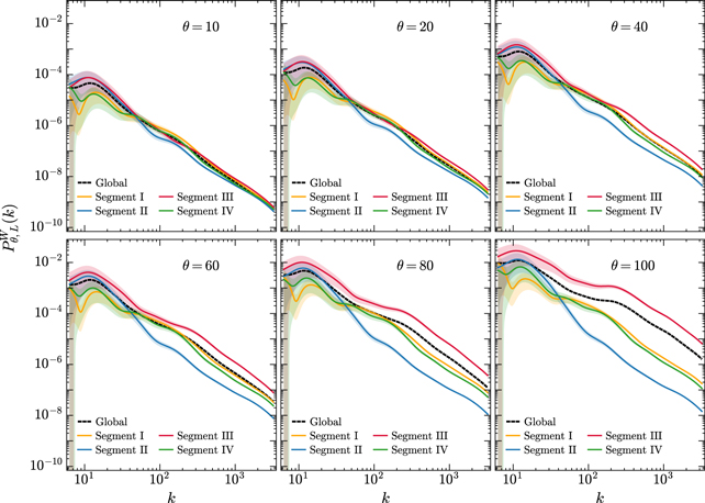
Figure 8. Local WPS for different density environments at times θ = 10, 20, 40, 60, 80, and 100. The shaded area for each curve represents the statistical error, from which we can see that those local WPSs are less significant statistically on scales of k ≲ 40.
Download figure:
Standard image High-resolution imageTable 2. Density Field at Each Time Split into Four Consecutive Segments a
| Segment | Spatial Range | Mean Density Contrast 
| |||||
|---|---|---|---|---|---|---|---|
| θ = 10 | 20 | 40 | 60 | 80 | 100 | ||
| I | 0.00 ≲ η ≲ 0.27 | 0.012 | 0.025 | 0.056 | 0.095 | 0.144 | 0.206 |
| II | 0.27 ≲ η ≲ 0.54 | −0.045 | −0.085 | −0.155 | −0.214 | −0.265 | −0.309 |
| III | 0.54 ≲ η ≲ 0.78 | 0.044 | 0.094 | 0.216 | 0.381 | 0.629 | 1.102 |
| IV | 0.78 ≲ η ≲ 1.00 | 0.000 | 0.001 | 0.007 | 0.018 | 0.037 | 0.066 |
Note.
a The spatial range spanned by each segment and the corresponding local mean density contrast at times of θ = 10, 20, 40, 60, 80, and 100 are listed.Download table as: ASCIITypeset image
In Figure 9, we also measure the local WPS at each time relative to its corresponding initial WPS within the scale range k ≳ 40 where statistical errors are smaller. For all segments, we see that  approximates to θ2 at stages of θ = 10 and 20. However, at late stages, the evolutionary trends of Segments II and III are completely opposite. For Segment II, the growth of small-scale components is getting slower, but for Segment III, the small-scale components are growing faster and faster. Although the WPSs of Segments I and IV are very similar, there are visible differences between them. Specifically, the former has a slightly upward tilt on small scales, while the latter remains roughly horizontal.

Figure 9. Local WPS for different density environments at times θ = 10, 20, 40, 60, 80, and 100 relative to the initial WPS.
Download figure:
Standard image High-resolution imageBased on these facts, we find that WPS is fully capable of detecting the effects of density environments on matter clustering. However, as pointed out above, the density field evolves into the nonlinear regime at late times, indicating that there are couplings between different scale components. The WPS, as two-point statistics, cannot determine such scale coupling since it does not contain phase information. To detect scale coupling, we measure the WBC, which is the lowest order statistics sensitive to nonlinear couplings between different scales of matter density field.
4.1.3. WBC Measurements
Figure 10 shows the time evolution of matter WBC with statistical noise subtracted, i.e., ![${b}_{\theta ,{L}_{b}}^{W}({k}_{1},{k}_{2})-\epsilon [{b}_{\theta ,{L}_{b}}^{W}({k}_{1},{k}_{2})]$](https://content.cld.iop.org/journals/0004-637X/934/1/77/revision1/apjac752cieqn41.gif) . Note that
. Note that  is symmetric about the diagonal where k1 = k2, as indicated by Equations (13) and (14). So we will only address the part below (or above) this diagonal. For visual convenience, values of bicoherence less than the noise level are not considered because they are less significant physically. To better understand the statistical noise level, as suggested by van Milligen et al. (1995a, 1995b), we perform FFT on the highly nonlinear density field at time θ = 100, and give each Fourier component a random phase while maintaining its amplitude, then we perform inverse FFT to get a new set of data. Such a new phase-randomized density field is expected to have no structures induced by scale coupling, while its power spectrum is identical to that of the raw density field, in which structures are well formed, as is illustrated in Figure 11. It can be seen that the summed WBC of the density field at θ = 100 is much higher than that of the phase-randomized version, which falls below the noise level along with the initial density field. Thus, the statistical noise level provides us a criterion to discriminate matter distributions with structures formed from those without. Accordingly, looking at Figures 10 and 11 together, there is a very weak coupling between large scales around k ∼ 10 and intermediate scales around k ∼ 300 at times θ = 10 and 20. Gradually, the scale coupling becomes more and more significant with time and eventually spreads to the entire scale range, which implies that the matter distribution becomes more and more structured.
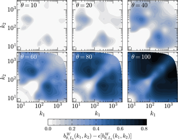
Figure 10. Contour plots of the WBCs with statistical noise level subtracted for density fields at times θ = 10, 20, 40, 60, 80, and 100. In these plots, values of the WBCs less than the statistical noise level are set to be zero.
Download figure:
Standard image High-resolution image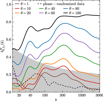
Figure 11. Summed WBC for density fields at times θ = 1, 10, 20, 40, 60, 80, and 100 (solid lines). The summed WBC for the phase-randomized data obtained from the density field at θ = 100 is indicated by the black dashed line and that of the initial density field (θ = 1) is indicated by the brown solid line as a comparison. The gray area represents the region where the summed WBC is less than the statistical noise level.
Download figure:
Standard image High-resolution imageIn Figure 12, we consider the evolution of the total WBC with time in the consecutive Segments I–IV. An interesting phenomenon is that the degree of nonlinearity in Segment II, the underdense region, is much higher than the noise level at the initial time, and this nonlinearity is less evolved. On the other hand, the nonlinearity is more evolved in overdense regions, although it is very weak at the initial time. In particular, Segment III, as a highly overdense region, has the strongest nonlinearity at late times. This implies that structure formation occurs mainly in Segment III. Furthermore, we examine the scale coupling for these segments by measuring their WBC and summed WBC at different times and corresponding results are shown in Figures 13 and 14. Consistent with the results in Figure 12, the estimated WBC and summed WBC in Segment II exhibit significant values between widely separated scales at the initial time because the matter distribution within such an underdense region is left-skewed. Both the WBC and summed WBC in Segment II barely evolve with time, indicating that there is almost no structure formation in this region. Also, Segment III shows a notable coupling between scale bands 20 ≲ k ≲ 100 and 100 ≲ k ≲ 500 at the initial stages, due to the matter distribution in such a highly overdense region being right-skewed. Unlike Segment II, the WBC and summed WBC of Segment III evolve the most dramatically, which indicates that the matter becomes increasingly clustered. For Segments I and IV, the bicoherences are below or close to the statistical noise level at the initial stages and evolve slowly with time, which means that the matter experiences moderate structure formation in these two slightly overdense regions.

Figure 12. Time evolution of the total WBC from the initial time θ = 1–100 in Segments I,–IV. The marker "N" indicates the noise level for each segment.
Download figure:
Standard image High-resolution image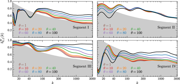
Figure 13. The summed WBC of four consecutive segments marked I–IV at times θ = 1, 10, 20, 40, 60, 80, and 100. The gray region of each subplot indicates where the summed WBC is below the statistical noise level.
Download figure:
Standard image High-resolution image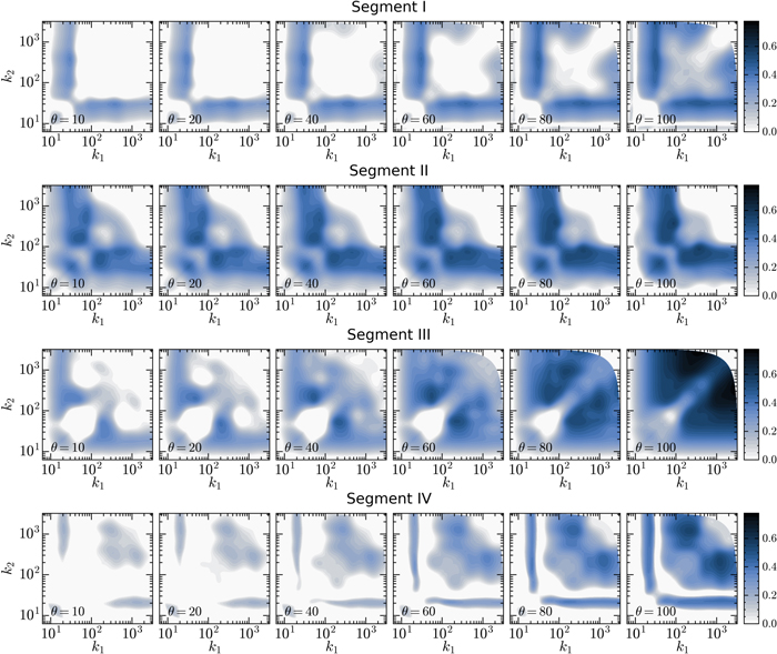
Figure 14. WBC with statistical noise subtracted, i.e., ![${b}_{\theta ,L}^{W}({k}_{1},{k}_{2})-\epsilon [{b}_{\theta ,L}^{W}({k}_{1},{k}_{2})]$](https://content.cld.iop.org/journals/0004-637X/934/1/77/revision1/apjac752cieqn43.gif) for local segments at times θ = 10, 20, 40, 60, 80, and 100. For an easier visual description, values of the WBC less than the statistical noise level are set to be zero in each subplot.
for local segments at times θ = 10, 20, 40, 60, 80, and 100. For an easier visual description, values of the WBC less than the statistical noise level are set to be zero in each subplot.
Download figure:
Standard image High-resolution image4.2. Wavelet Analysis of the Density Fields of the TNG100 Simulation
In previous sections, we focused on the wavelet analysis of the nonlinear evolution of the 1D Zel'dovich density field, revealing the considerable potential of the CWT for characterizing the matter clustering. Therefore, we further apply the 3D continuous wavelet method to the analysis of the TNG100 simulation. For simplicity, we consider the 3D isotropic CWT methods based on the GDW described in Appendix B, which is the simplest extension of the 1D case. We first perform the isotropic CWT of the 3D density fields of the total matter, DM, gas, and stars
6
at redshift z = 0. In order to avoid the aliasing, we take the maximum scale as  , where kNyq =1024π/Lbox is the Nyquist frequency of the density grid. For the purpose of presentation, WTs of density slices at three scales are shown in Figure 15. By visual inspection, We see that for all matter components, only large voids and filaments are captured at the large scale of k ≈ 0.35 hMpc−1, whereas as the scale becomes smaller, the WT is increasingly accurate in tracking the finer web-like structure of the universe. More quantitative statements can be made by using statistics formulated on the WT.

Figure 15. 2D slices of density fields δf
(r) + 1 and their WT Wf
(k, r), where f stands for the total matter, DM, gas, and stars from top to down, respectively. These slices are 75 × 75 h−2Mpc2, with a thickness of 73.242 h−1 kpc (one cell scale). The left panels show the density fields at redshift z = 0, and the next panels are their wavelet coefficients at scales k ≈ 0.35, 0.90, and 6.08 hMpc−1, respectively. Notice that the wavelet scale w is replaced by its equivalent Fourier wavenumber k according to the relation  , which is obtained following the method in Section 2.5.
Download figure:
Standard image High-resolution imageIn Figure 16, we compare the global wavelet and Fourier power spectra for different matter distributions. It can be seen that these two types of spectra for each matter have a similar shape. The global WPS of the total matter falls slightly below that of the DM at small scales. The gas becomes significantly less clustered than DM at intermediate and small scales, while the stellar mass shows a very strong clustering. However, the magnitude of the WPS is different from the Fourier power spectrum. More precisely, the deviations between these two spectra are measured by the ratio between them, which appears to be roughly a constant determined by Equation B13.
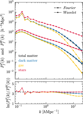
Figure 16. Top panel: the global wavelet and Fourier power spectra for different matter components at redshift z = 0. We show results for the total matter, DM, gas, and stars, as labeled. Bottom panel: the ratio between the global WPS and Fourier power spectrum for each matter component. The horizontal dashed line denotes the constant  given by Equation (B13).
Download figure:
Standard image High-resolution imageTo study the impact of a large-scale environment on the matter clustering, we divide the whole simulation volume  into
into  sub-volumes of
  , where Nsub is set to be 8 and hence the side length Lb
/Nsub is 9.375 h−1Mpc. In Figure 17, we show the local WPSs of the total matter spatial distribution measured in the sub-volumes. These local WPSs are separated into six categories, according to the mean densities of sub-volumes as follows:
, where Nsub is set to be 8 and hence the side length Lb
/Nsub is 9.375 h−1Mpc. In Figure 17, we show the local WPSs of the total matter spatial distribution measured in the sub-volumes. These local WPSs are separated into six categories, according to the mean densities of sub-volumes as follows:
- 1.
 ,
, - 2.,
- 3.,
- 4.,
- 5.,
- 6.,


where  denotes the local mean density of the total matter within a sub-volume. We see that the local WPSs are greater for sub-volumes with higher local mean density for scales up to a few times 0.1 hMpc−1. To make it more explicit, we consider the mean of the local WPSs over all sub-volumes within each density interval, which is shown below:

where the density interval  is specified by the abovementioned list (i)–(vi). These results are presented in Figure 18. Obviously, at the largest scales,
  in all density intervals converge to the global WPS, while as scales become smaller, discrepancies between
  in different density intervals as well as the global WPS become more pronounced. We noticed that the mean local WPS in
  is the most enhanced among all density intervals, particularly at scales around 3 hMpc−1, where they are dominated by the most massive halos, as pointed out by van Daalen & Schaye (2015). As the local mean density
  gets smaller, the mean local WPS gets smaller. In
  , the mean local WPSs are most severely suppressed on scales of k ∼ 3 hMpc−1. Therefore, our results suggest that most massive halos tend to reside in the densest environments, while those less dense environments show a deficit of massive halos, which are qualitatively consistent with the results of Fisher & Faltenbacher (2018) and Zhu et al. (2022).

Figure 17. Local WPSs of the total matter  measured from
  sub-volumes of V = 9.3753
h−3Mpc3. The color represents the local mean density
sub-volumes of V = 9.3753
h−3Mpc3. The color represents the local mean density  of each sub-volume.
Download figure:
Standard image High-resolution image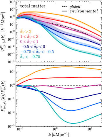
Figure 18. Top panel: the mean of local WPSs in each density interval for the total matter distribution. The shaded regions represent the standard deviations for the values above and below the mean calculated separately. As a comparison, the global WPS of the total matter distribution is indicated by the dashed line. Bottom panel: the ratio of the mean local WPS in each density interval relative to the global WPS.
Download figure:
Standard image High-resolution imageNote that the total matter density field is formed via

Combining this equation and Equation (B6), the local WPS of the total matter in a sub-volume can be separated into

in which the cross terms  encode the coherence between different matter species. This can be examined by the local WCC
  , which is defined as Equation (B7). The mean values of local WCCs in different density intervals
  are shown in Figure 19. On large scales,
  is close to one for all pairs of matter components in all density environments, whereas it deviates more from one on smaller scales, and also shows more distinct discrepancies between different density environments. Specifically, in
  , the correlation between the DM and stars remains higher than other pairs on scales of k ≳ 3 hMpc−1. However, this correlation decreases with decreasing density. This could be explained by the fact that stars are mostly formed in the center of halos, which are very few in less dense environments. For the DM and gas pair, the correlation between them is very close to 1 and hardly varies with the density environment on the scales of k ≲ 2 hMpc−1. On scales smaller than 2 hMpc−1, this correlation first decreases with decreasing density until reaching the minimum in
  and then increases with decreasing density, so that it becomes even higher than that between the DM and stars in
  . For the gas and star pair, the correlation between them shows a density dependence similar to that between the DM and gas, but it is still lower than other pairs of matter in all density environments. Within the scale range we investigate, the variation of gas-DM and gas-star correlations with scale and density may be related to the feedback processes, mainly active galactic nuclei (AGNs) feedback at z = 0, which can expel gas from halos to large distances and hence reshape the matter distribution.
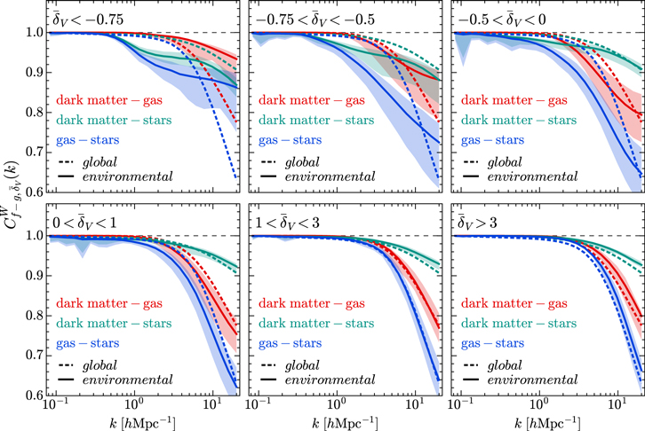
Figure 19. The mean of local WCCs in different density intervals  , where f and g stand for DM, gas or stars, respectively. The color areas represent the standard deviations for the values above and below the mean calculated separately. The global WCCs are indicated by the dashed lines for reference.
Download figure:
Standard image High-resolution imageIn order to investigate the impact of the AGN feedback on the matter clustering in different density environments, we consider the ratio between the local WPS from TNG100-1 and that from the corresponding DM-only simulation TNG100-1-Dark, i.e.,  , where f refers to the total matter, DM, and total baryons (gas+stars), respectively. The mean values of
  in different density intervals are plotted in Figure 20. For the total matter, we see that its global WPS is reduced on scales k ≳ 1 hMpc−1 relative to the DM-only's global WPS, with a 14% suppression at k ∼ 20 hMpc−1. This effect is also seen in the local WPS, but with some variation in different density environments. The change in the total matter clustering compared to that in the DM-only simulation comes from two aspects: (1) the redistribution of baryons by nongravitational physics, and (2) the change in the DM distribution resulted from the gravitational coupling of baryons and DM, which is called the back reaction (van Daalen et al. 2020). We see from Figure 20 that the former effect is the determinant of the change in the clustering of total matter for all density intervals. In particular, the clustering strength of baryons is the least suppressed in the density ranges of
  and
and  , revealing that the AGN feedback is the weakest in the densest and most underdense environments. Considering the fact that most massive halos prefer to reside in the densest environments, our results are consistent with the findings of Springel et al. (2018), showing that AGN feedback has a minimal impact on the most massive halos. As for the lowest AGN feedback in the most underdense environments, it may be related that these environments contain few or no halos.
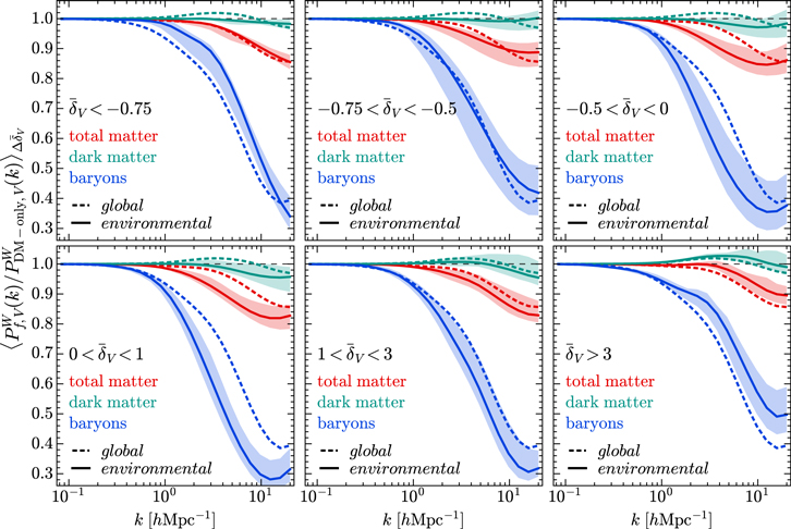
Figure 20. The mean of the ratio between the local WPSs of the total matter, DM, and baryons (gas+stars) from the TNG100-1 and the local WPS from the corresponding DM-only simulation TNG100-1-Dark in different density intervals. The color areas represent the standard deviations for the values above and below the mean calculated separately. The ratio between the global WPSs is indicated by the dashed lines for reference.
Download figure:
Standard image High-resolution image5. Discussion and Conclusions
The clustering of matter is an intricate process. In addition to redshift and scale dependence, the density environment plays a very important role in the clustering. When the usual Fourier statistics are utilized to examine the scale dependence, we are unable to take into account the effect of the environment, since the local density information contained in the physical space is smeared out. Therefore, we need better tools to consider the dependence of both scale and environment simultaneously, and the continuous WT is such a tool with good performance.
In this work, we introduce some statistical quantities formulated on the specific wavelet function, GDW, which is a real valued continuous wavelet designed by taking the first derivative of the Gaussian smoothing function with respect to the scale parameter. With such a wavelet construction scheme, the original signal can be recovered from wavelet coefficients easily. These wavelet statistics we used include the WPS, the WCC, and the WBC.
To reveal the usefulness of wavelet statistics in analyzing matter clustering, we analyze the time evolution of the 1D density distributions obtained from the Zel'dovich approximation by measuring their wavelet power spectra and bicoherences. Measurements show that the global WPS on small scales increases more significantly with time than that on large scales, which is generally in agreement with the Fourier case.
To manifest the capability of wavelet statistics to perform local spectral analysis, we divide the 1D Zel'dovich density field at each time into four consecutive segments. All the local wavelet power spectra for these segments almost converge to the global WPS at linear stages. However, the difference between the local power spectra and the global WPS becomes progressively larger with time due to nonlinear effects. In particular, the WPS of Segment III (highly overdense environment) is significantly greater than those of the other segments on scales k ≳ 40, where statistical errors are smaller, which implies that structures on these scales are generated in this region at nonlinear stages. Another striking feature is that the growth of the WPS in Segment II (underdense environment) is severely suppressed on scales k ≳ 40, meaning that there are very few structures on these scales generated in this region at later times. Moreover, measurements of the WBCs show that the scale coupling occurs mainly in Segment III, whereas there is almost no scale coupling in Segment II at late epochs. Both the WPS and the WBC in Segments I and IV exhibit similar behaviors to and fall between those in Segments II and III, probably because Segments I and IV are slightly overdense environments. These results demonstrate the great potential of wavelet statistics for taking into account the effects of both environment and scale on matter clustering.
Furthermore, we generalize the 1D CWT methods to the 3D isotropic version and apply them to the 3D density fields of the TNG100-1 simulation at redshift z = 0. Due to space limitations, WBCs of the 3D density fields are left for future works. In order to examine the impact of the large-scale environment on the matter clustering, we split the whole simulation volume evenly into 512 small cubes and then measure the local WPS and WCC for different matter species in each sub-volume. To clearly see the dependence of the matter clustering on the density environment, we consider the mean of local WPSs and WCCs over all sub-volumes within each density interval. Our main findings are summarized as follows:
- 1.On the largest scales, the clustering of the total matter shows no dependence on the density environment, whereas it increases monotonically with increasing density on scales up to several times 0.1 hMpc−1. Compared to the global WPS of the total matter, its mean local WPS is most enhanced in the density of around scales of 3 hMpc−1 where it is dominated by the most massive halos. As the density becomes smaller and smaller, the mean local WPS is more and more suppressed around scales of 3 hMpc−1, suggesting that lower density environments contain less massive halos.
- 2.For the pairs of the DM gas, DM stars, and gas stars, the cross correlations in all density environments are close to one on large scales, whereas they deviate from one significantly on small scales. Specifically, we find that the DM and stars are less correlated in less dense environments on small scales. The correlation between the DM and gas remains close to one in all environments on the scales of k ≲ 3 hMpc−1. On smaller scales, this correlation first decreases and then increases with the increasing density. The correlation between the stars and gas also shows a similar density dependence, but is lower than other pairs.
- 3.As revealed by the ratio between the local WPS from the TNG100-1 and that from its companion DM-only simulation, the impact of the AGN feedback on the matter clustering also varies with the density environment. Particularly, AGN feedback has less impact on the matter clustering in the densest environments and the most underdense environments . Compared to these extreme environments, the matter clustering strength at small scales is more suppressed by the AGN feedback in densities of .


These results are qualitatively consistent with previous research on matter clustering (e.g., van Daalen & Schaye 2015; Fisher & Faltenbacher 2018; Springel et al. 2018; van Daalen et al. 2020; Zhu et al. 2022). This encourages us that we can further apply statistics based on the continuous WT to various cosmological simulations and characterize the environmental dependence of the matter clustering and the baryonic effects on it in more detail.
Y.W. especially thanks Dr. van Milligen for helpful discussions on the statistical error estimation for wavelet statistical quantities. P.H. acknowledges the support of the Natural Science Foundation of Jilin Province, China (No. 20180101228JC), and by the National Science Foundation of China (Nos. 12047569, 12147217). In this work, we used the data from IllustrisTNG simulations. The IllustrisTNG simulations were undertaken with computing time awarded by the Gauss Centre for Supercomputing (GCS) under GCS Large-Scale Projects GCS-ILLU and GCS-DWAR on the GCS share of the supercomputer Hazel Hen at the High Performance Computing Center Stuttgart (HLRS), as well as on the machines of the Max Planck Computing and Data Facility (MPCDF) in Garching, Germany.
Appendix A: Choice of the Wavelet
In principle, there is a diverse set of wavelets available in the CWT. For instance, the most common ones are the Poisson wavelet, the Mexican hat wavelet, the spline wavelet, the Meyer wavelet, and the Morlet wavelet (see, e.g., Akujuobi 2022 for a review of wavelets). The choice of an appropriate wavelet depends on the goal of the performed analysis. In this study, we chose to use the GDW for two reasons. First, its shape matches well that of the density peak. Second, it provides a good trade-off between spatial and frequency resolution. Subsequently, we will highlight the superiority of the GDW by comparing it with the Poisson and Morlet wavelets.
The Poisson wavelet described by (Holschneider 2000) is
with Fourier transform

where the constant CPoi is used to make it have the same energy as the GDW. As can be seen from Figure A1, the Poisson wavelet is more localized in the spatial domain but less localized in the frequency domain than the GDW is. The Morlet wavelet (also called the Gabor wavelet) given by Hong & Kim (2004) is written as

which is a harmonic function with frequency η modulated by a Gaussian envelope with variance σ2, and its Fourier transform is

where the constant CMor is used to make it have the same energy as the GDW. In principle, the Morlet wavelet is not a true wavelet function, since it does not satisfy the admissibility condition, i.e.,  is infinite. This means that the Morlet WT has no inverse transform (Daubechies 1992). Only when ∣σ
η∣ is large enough, the admissibility condition is approximately satisfied. A reasonable choice would be ∣σ
η∣ ≥ 5 (Hong & Kim 2004), and here we set σ = 5, η = −1. In this case, compared to the GDW and the Poisson wavelet, the Morlet wavelet is the most extended in the spatial domain but the narrowest in the frequency domain, as shown in Figure A1.
is infinite. This means that the Morlet WT has no inverse transform (Daubechies 1992). Only when ∣σ
η∣ is large enough, the admissibility condition is approximately satisfied. A reasonable choice would be ∣σ
η∣ ≥ 5 (Hong & Kim 2004), and here we set σ = 5, η = −1. In this case, compared to the GDW and the Poisson wavelet, the Morlet wavelet is the most extended in the spatial domain but the narrowest in the frequency domain, as shown in Figure A1.

Figure A1. Top panel: the GDW, Poisson wavelet, and Morlet wavelet. Bottom panel: the respective Fourier transforms of the wavelets in the top panel.
Download figure:
Standard image High-resolution imageIn order to discern the applicability of the discussed wavelets, we use them individually to calculate the squared CWT of the 1D Zel'dovich density field at θ = 100, which is shown in Figure A2. We observe that in the Poisson case, structures of the density field are resolved quite well along the spatial axis, whereas they are very poor along the scale axis. The Morlet wavelet yields the best separation of scales but the worst separation of spatial features among these wavelets. The GDW performance is intermediate between the Poisson and the Morlet wavelets, giving moderate spatial and scale resolution. Therefore, using GDW to perform local spectral analysis may provide more reliable results.
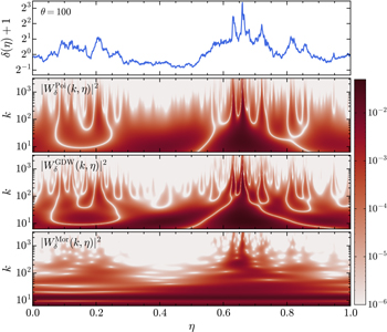
Figure A2. First panel: the 1D density field at θ = 100 obtained through Equation (23). Second panel: the squared WT  of the density field based on the Poisson wavelet, where
  . Here the scaled Poisson wavelet is defined as
  , and the relation k = 3w/2 is obtained following the method in Section 2.5. Third panel: same as the second panel, but using the GDW. Fourth panel: same as the second panel, but using the Morlet wavelet. For this wavelet, the relationship between the scale parameter and the corresponding Fourier wavenumber is
  .
.
Download figure:
Standard image High-resolution imageAppendix B: 3D Isotropic GDW and CWT
In general, the 3D CWT uses a scale vector containing three scale parameters, i.e., w = (wx , wy , wz ), which measures the scale along each of the three axes (x, y, and z), as pointed out by Wang & He (2021). For simplicity, we consider the isotropic case, in which the same scale parameter w is used for all directions. Then the isotropic CWT of the 3D field is written as

where  represents the 3D real space, and Ψ(w, r) is the isotropic GDW, which is defined by
where  is the isotropic Gaussian smoothing function, and the index κ is set to be −1/2 so that the integral ∫∣Ψ(w, r)∣2d3
r is constant. The Fourier transform of the isotropic GDW is
is the isotropic Gaussian smoothing function, and the index κ is set to be −1/2 so that the integral ∫∣Ψ(w, r)∣2d3
r is constant. The Fourier transform of the isotropic GDW is

In line with the method used to obtain Equation (6), combining Equations (B1) and (B2) yields the inverse CWT,

Recalling that the 1D wavelet-based statistics are defined through the integral over a length L, the 3D wavelet-based statistics can be defined through the integral over a volume V = L3. The local WPS defined in this way is shown below:

which is the volume average of squared wavelet coefficients within the local volume V, and hence can be written in a more compact form as

Then the local WCC between two fields, f(r) and g(r), is given by
where  .
.
For simulated cosmic fields with a periodic box of volume  , the global WPS is obtained by replacing the local volume V with the total volume Vb
,
, the global WPS is obtained by replacing the local volume V with the total volume Vb
,

and the global WCC is

where  . In the 1D case, the global WPS is a smoothed version of the Fourier power spectrum, as stated in Section 2.3. Here we go further and give a tighter relationship between the wavelet and the Fourier power spectra. According to Parseval's theorem, we have
in which we exploit the fact that GDW is isotropic, namely,  . If
. If  is also isotropic, then the above equation has a more simple form,

where  is the Fourier power spectrum. Integrating the scale factor w at both ends of this equation yields

in which  . Finally, with the help of the relation
  obtained by following the method in Section 2.5, we find that the global wavelet and Fourier power spectra differ by only one constant factor, as shown below:

Footnotes
- 3
In Wang & He (2021), we simply define GDW as ψ(w, x) ≡ ∂G(w, x)/∂w.
- 4
A detailed comparison between the GDW and the Mexican hat wavelet is given in Wang & He (2021).
- 5
Following the same logic, the relation between the wavelet scale and its equivalent Fourier wavenumber is
for the 3D isotropic CWT. - 6
Similar to what Springel et al. (2018) did in measuring the cross-correlation functions between different matter, we here put the black holes and stars together, and then labeled them as stars.
