


Abstract
The cosmic formation rate of long gamma-ray bursts (LGRBs) encodes the evolution, across cosmic times, of the properties of their progenitors and of their environment. The LGRB formation rate and the luminosity function, with its redshift evolution, are derived by reproducing the largest sets of observations collected over the last four decades, namely the observer-frame prompt emission properties of the GRB samples detected by the Fermi and Compton Gamma Ray Observatory satellites and the redshift, luminosity, and energy distributions of the flux-limited, redshift-complete samples of GRBs detected by Swift. The model that best reproduces all these constraints consists of a GRB formation rate increasing with redshift ∝(1 + z)3.2, i.e., steeper than the star formation rate, up to z ∼ 3, followed by a decrease ∝(1 + z)−3. On top of this, our model also predicts a moderate evolution of the characteristic luminosity function break ∝(1 + z)0.6. Models with only luminosity or rate evolution are excluded at >5σ significance. The cosmic rate evolution of LGRBs is interpreted as their preference for occurring in environments with metallicity  , consistent with theoretical models and host galaxy observations. The LGRB rate at z = 0, accounting for their collimation, is
  Gpc−3 yr−1 (68% confidence interval). This corresponds to ∼1% of broad-line Type Ibc supernovae producing a successful jet in the local universe. This fraction increases up to ∼7% at z ≥ 3. Finally, we estimate that at least ≈0.2−0.7 yr−1 of the Swift- and Fermi-detected bursts at z < 0.5 are jets observed slightly off-axis.
Export citation and abstract BibTeX RIS

Original content from this work may be used under the terms of the Creative Commons Attribution 4.0 licence. Any further distribution of this work must maintain attribution to the author(s) and the title of the work, journal citation and DOI.
1. Introduction
The distinctive features of long-duration gamma-ray bursts (LGRBs)—such as their detection up to high redshifts (z = 8.2–9.2; Salvaterra et al. 2009; Tanvir et al. 2009; Cucchiara et al. 2011), their association with faint blue star-forming galaxies, their positional coincidence with the brightest ultraviolet regions within their hosts (Fruchter et al. 2006), and their association with core-collapse supernovae (Hjorth & Bloom 2012)—point to a massive-star progenitor, thus establishing a direct link with the formation and relatively rapid evolution of massive stars across cosmic times. The study of increasingly larger samples of hosts has revealed the preference of LGRBs to form in subsolar-metallicity environments (Vergani et al. 2015; Perley et al. 2016; Palmerio et al. 2019). This is in agreement with the progenitor model (MacFadyen & Woosley 1999) requiring a low metallicity to maintain a high specific angular momentum at the time of the core collapse, in order to produce the GRB jet (Yoon et al. 2006). Therefore, the physical conditions for the production of a relativistic jet determine the intrinsic properties of the LGRB population, such as their characteristic luminosities and cosmic rates.
GRB population studies aim at reconstructing the population luminosity and formation rate functions. The free parameters of these functions are often constrained by reproducing sets of rest-frame and observer-frame properties (Daigne et al. 2006; Wanderman & Piran 2010; Robertson & Ellis 2012) of the detected GRB samples and properly accounting for sample incompleteness (Salvaterra et al. 2012; Ghirlanda et al. 2015; Palmerio & Daigne 2021).
In this work, we build a GRB population model (Section 2) and derive the cosmic formation rate of LGRBs and their luminosity function, together with its evolution with redshift. To this end, we exploit, for the first time, the largest set of observational constraints collected by different GRB detectors over the last four decades (Section 3). We account for the presence of relativistic jets and the orientation-dependence of the observed GRB properties. We derive the evolution of the ratio of the GRB formation rate to the cosmic star formation rate (CSFR), and test its consistency with the host metallicity bias (Section 4). We discuss the implications of our population model in Section 5. Throughout the paper, we assume a standard flat cosmology, with ΩM = 0.3 and h = 0.7.
2. The Model
We build a synthetic LGRB population model, based on two distribution functions. The GRB formation rate per unit of comoving volume ρ(z) is modeled with the parametric function (Cole et al. 2001; Madau & Dickinson 2014)
where ρ0, in Gpc−3 yr−1, is the LGRB local density rate. The choice of this functional form is motivated by its relatively small number of free parameters and, for ease of comparison, by its systematic use for fitting the CSFR (Madau & Dickinson 2014; Madau & Fragos 2017; Hopkins & Beacom 2006). Flat priors are considered for the free parameters (pz,1, pz,2, and pz,3) that can vary over wide ranges, also including the values corresponding to the CSFR. This ensures that we can recover, if present, any significant deviation of the GRB formation rate from the CSFR.
The luminosity function of LGRBs is often described in the literature by a broken power law (e.g., Salvaterra et al. 2009; Salvaterra et al. 2012):
where a1 and a2, respectively, are the indices of the power laws below and above the break luminosity Liso,b, which is left free to evolve with redshift ∝(1 + z)δ . Therefore, Liso,0 represents the break of the luminosity function at z = 0. Φ(Liso, z) is normalized to its integral and it is defined for Liso ≥ 1047 erg s−1. An alternative working hypothesis sometimes considered in the literature is the Schechter (Schechter 1976) luminosity function. We discuss in Appendix A.3 the results obtained under this different assumption. In summary, our model allows for the evolution of the GRB population both in terms of rate density (Equation (1)) and luminosity (Equation (2)).
LGRBs follow the Ep − Liso (Yonetoku et al. 2004) correlation, where Ep is the peak energy of the ν Fν
spectrum and the Ep − Eiso correlation (Amati & Frontera 2002) links the peak energy with the isotropic energy Eiso. It has been proved (Nava et al. 2012; Dai et al. 2021) that these correlations do not evolve with redshift. Following Ghirlanda et al. (2015), in our simulation we sample Equation (1), extracting a redshift, and we independently assign an Ep value sampling a broken power law. The values of Liso and Eiso corresponding to Ep are derived from the Ep − Liso and Ep − Eiso correlations, respectively, accounting for their Gaussian scatters (Nava et al. 2012). For ease of comparison with the literature, once we have derived the posterior parameter distributions of the model, we map, through the Ep − Liso correlation, the peak energy distribution function back to the luminosity function, and we provide the resulting parameter values in Table 1. GRB rest-frame durations are estimated as f · Eiso/Liso, where f is a scaling factor sampled from a free Gaussian distribution ![${\mathfrak{G}}[f| \mu ,\sigma ]$](https://content.cld.iop.org/journals/0004-637X/932/1/10/revision1/apjac6e43ieqn3.gif) .
.
Table 1. Parameters of the GRB Population Model
| ρ(z) |

|

|

|
 Gpc−3 yr−1 Gpc−3 yr−1
| ⋯ |
|---|---|---|---|---|---|
| Φ(Liso, z) |

|

|
|

| ⋯ |
![${\mathfrak{G}}[\mathrm{log}f| \mu ,\sigma ]$](https://content.cld.iop.org/journals/0004-637X/932/1/10/revision1/apjac6e43ieqn12.gif)
|

|

| ⋯ | ⋯ | ⋯ |
![${\mathfrak{G}}[\alpha | \mu ,\sigma ]$](https://content.cld.iop.org/journals/0004-637X/932/1/10/revision1/apjac6e43ieqn15.gif)
| μ = −1.0 | σ = 0.1 | ⋯ | ⋯ | ⋯ |
![${\mathfrak{G}}[\beta | \mu ,\sigma ]$](https://content.cld.iop.org/journals/0004-637X/932/1/10/revision1/apjac6e43ieqn16.gif)
| μ = −2.3 | σ = 0.1 | ⋯ | ⋯ | ⋯ |
| K | S | Σ | Y0 | X0 | |
 Eiso-
Eiso-  θjet
θjet
|

|

| 0.1 | 1 | 1 |
 Ep-
Ep-  Liso
Liso
| 0.27 | 0.56 | 0.18 | 406.7 | 3.38 × 1052 |
 Ep-
Ep-  Eiso
Eiso
| −0.12 | 0.58 | 0.20 | 406.7 | 9.10 × 1052 |
 Γ0- Γ0-  Eiso
Eiso
| 2.1 | 0.3 | 0.1 | 1 | 1052 |
Note. The parameters constrained through the MCMC (Section 2) are reported with the associated 1σ uncertainty. Their posterior distributions are shown in Figure 2. The parameters without errors are held constant. The four correlations listed are expressed in the form  , with the parameter Σ representing their scatter along the independent coordinate. Eiso, Liso, Ep, and θjet have units of erg, erg s−1, keV, and rad, respectively.
Download table as: ASCIITypeset image
It is known that GRBs are highly collimated (e.g., Ghirlanda et al. 2007). Therefore, we compute their intrinsic rate ρ(z) (Equation (1)) by accounting for the elusive bulk of the population consisting of events with jets oriented to the side of our line of sight. We assume uniform conical jets distributed with random orientations θv with respect to the line of sight. The jet opening angle values θjet appear to be correlated with Eiso (Ghirlanda et al. 2007), such that we assume a free parametric correlation θjet–Eiso. Even off-axis jets (θv > θjet) may be detected, depending on their orientation and bulk Lorentz factor Γ, characterizing the prompt emission phase. We account, for the first time within a population study of LGRBs, for the relativistic effects on the observed flux and fluence, as well as the peak energy induced by the jet orientation and the beaming through the Doppler factor  (see, e.g., Ghisellini et al. 2006). To this end, we sample the Γ–Eiso correlation reported by Ghirlanda et al. (2018), to assign Γ values to the simulated events.
The GRB prompt emission spectrum is described with the empirical Band function (Band et al. 1993), consisting of two smoothly joined power laws. To each simulated GRB we assign a low- and high-energy spectral index, extracted from the Gaussian distributions ![${\mathfrak{G}}[\alpha | \mu ,\sigma ]$](https://content.cld.iop.org/journals/0004-637X/932/1/10/revision1/apjac6e43ieqn29.gif) and
and ![${\mathfrak{G}}[\beta | \mu ,\sigma ]$](https://content.cld.iop.org/journals/0004-637X/932/1/10/revision1/apjac6e43ieqn30.gif) , respectively, whose parameters (e.g., Goldstein et al. 2012) are given in Table 1.
, respectively, whose parameters (e.g., Goldstein et al. 2012) are given in Table 1.
The population model has 12 free parameters (Table 1): [ρ0, pz,1, pz,2, pz,3] describe the GRB cosmic formation rate (Equation (1)) and [a1, a2, Liso,0, δ] define the luminosity function (Equation (2)); the remaining four parameters (μ, σ) and (K, S) describe the stretching factor of the duration distribution and the Eiso–θjet correlation, respectively. All the other parameters reported in Table 1 are fixed to their presently known values and are derived from the corresponding references given above.
The 12 free parameters are constrained by matching a set of observed distributions CJ (Section 3) and by maximizing a binned likelihood. The probability that the model distribution has mi objects in the i bin of the distribution, given that there are ri real events in this bin, follows a Poisson distribution. The total log-likelihood can be expressed as
where the internal sum is performed over n bins of each distribution of the constraint CJ (with J = 1,...,14). The observational constraint distributions CJ (described in Section 3) are built from the observed properties of the LGRB samples detected by different instruments, and are represented by the different symbols in the panels of Figure 1.
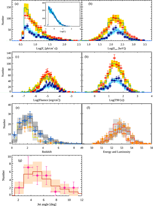
Figure 1. Observational constraints of the model population. Panel (a): distributions of peak flux on a 1.024 s timescale integrated over the 10–1000 keV energy range for Fermi/GBM (red circles) and CGRO/BATSE (blue squares) GRBs, with Fp ≥ 4 ph cm−2 s−1. The inset shows the peak flux (50–300 keV) of the BATSE GRBs reconstructed by an offline search (Stern et al. 2001), with Fp ≥ 0.3 ph cm−2 s−1. Panels (b), (c), and (d) show the Ep, fluence F (10–1000 keV), and T90 distributions (for GBM and BATSE, with the red circles and blue squares, respectively). Panel (e) shows the redshift distributions of the Swift BAT6 complete sample (orange circles) and the Swift SHOALS sample (blue stars), while panel (f) shows the Liso and Eiso (open squares and filled circles, respectively) distributions of the BAT6 sample. Panel (g) shows the jet opening angle distribution (circles). In each panel, the solid-line histogram and the shaded (dashed) region show the best model and its 1σ uncertainty, respectively, as obtained by the MCMC method described in Section 2. The model uncertainty is obtained by sampling the posterior distributions of the free parameters (shown in Figure 2) and including Poisson uncertainty.
Download figure:
Standard image High-resolution imageThe posterior distributions of the 12 free parameters are derived through a Markov Chain Monte Carlo (MCMC) method, which samples from wide uniform prior distributions of the free parameters: pz,1 ∈ [1, 6], pz,2 ∈ [0.1, 6], pz,3 ∈ [1, 9], δ ∈ [0, 5], a1 ∈ [0.5, 3], a2 ∈ [2, 5], logLiso,b ∈ [50, 53], μf ∈ [1.5, 10], σf ∈ [0.01, 6], KE−θ ∈ [9, 10.5], and SE−θ ∈ [ −0.25, −0.1]. We implement the Goodman & Weare (2010) MCMC algorithm. We work with 200 walkers running over 200 steps, and we adopt the parallel stretch move method (Foreman-Mackey et al. 2013) to reduce the computation time.
3. Observational Constraints
The free parameters of the GRB population model are constrained by reproducing a set of distributions of the observables provided by samples of GRBs detected by different missions. The numerous samples of LGRBs detected by the Gamma Burst Monitor (GBM) on board the Fermi satellite and the Burst And Transient Source Experiment (BATSE) on board the Compton Gamma Ray Observatory (CGRO) provide the peak flux (FP ) and fluence (F) distributions (panels (a) and (c) of Figure 1), as well as the observer-frame peak energy (Ep/1 + z) and duration (T90) (panels (b) and (d) of Figure 1). In order to minimize sample incompleteness, which is particularly severe at the faint end of the peak flux distribution, 4 we consider LGRBs with FP ≥ 4 ph cm−2 s−1, integrated over the 10 keV–1 MeV energy range for Fermi/GBM and the 20 keV–2 MeV range for GCRO/BATSE. This selection results in 904 GRBs (out of 1906) for Fermi/GBM (the red symbols in Figure 1) and 370 (out of 1529) for CGRO/BATSE (the blue symbols in Figure 1). The inset in Figure 1(a) shows the peak flux (50–300 keV) of 2810 CGRO/BATSE bursts in the Stern et al. (2001) catalog, with Fp ≥ 0.3 ph cm−2 s−1.
For the redshift distribution (panel (e)), we consider two well-selected Swift/BAT flux-limited samples, in which large majorities of the bursts have a redshift measurement. The BAT6 sample (Salvaterra et al. 2012; Pescalli et al. 2016) consists of LGRBs with a 15–150 keV peak flux ≥2.6 ph cm−2 s−1. The SHOALS sample (Perley et al. 2016) comprises GRBs with a 15–150 keV integrated fluence ≳10−6 erg cm−2. Both these samples have 80%–90% redshift measurements, either from afterglow or host spectroscopy. The BAT6 sample also provides the constraints on the Eiso and Liso distributions (panel (f)). Finally, we consider the jet opening angle distribution (panel (g)) of the GRBs collected in Ghirlanda et al. (2007).
Further, we also verified the consistency of our best model (Figure 5 in Appendix A.1) with the distributions of the peak flux, fluence, and duration (T90) of the samples of LGRBs observed by Swift/BAT 5 and the Gamma Ray Burst Monitor (GRBM) on board the Beppo/SAX satellite (Frontera et al. 2008).
4. Results
The model that best matches the set of observational constraints is shown by the solid histograms in Figure 1 (and in Figure 5). The shaded/dashed regions around the model line represent the 68% model uncertainty. This is computed by resampling the joint posterior distributions of the free parameters (shown in Figure 2) with 105 samples, then computing the corresponding model for each. For each fixed value of an independent variable, the shaded region shows the 16th to 84th percentile of the resulting model. The posterior distributions of the best model are shown by the corner plot in Figure 2, and their central values and 1σ uncertainty are reported in Table 1. All the parameter values are well constrained with, on average, ∼10% accuracy.
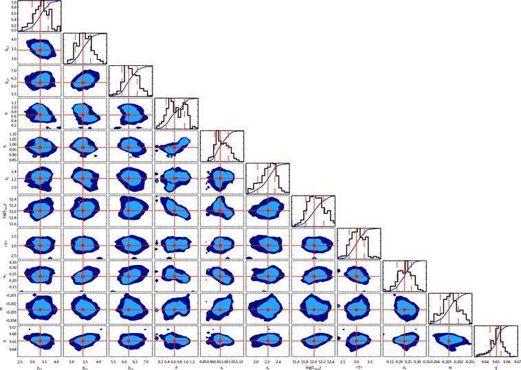
Figure 2. Corner plot showing the posterior distributions of the 12 free model parameters. The positions of the mean values of the distributions are represented by the red circles and the solid red lines in the two-dimensional plots. The shaded contours for each couple of parameters represent the 68% and 95% contours (light and dark blue, respectively). The main diagonal plots show the histograms of the posterior values of each free parameter (with the cumulative normalized distribution shown as a thin blue line), and the solid and dashed red lines mark the central value and 68% confidence interval, respectively.
Download figure:
Standard image High-resolution imageThe luminosity function has a faint-end slope ∼ −1 and a bright-end slope ∼ −2.2, with a break in luminosity at z = 0 Lb,0 = 1052 erg s−1. These values are consistent with those reported by previous studies (Wanderman & Piran 2010; Salvaterra et al. 2012). We find a mild evolution of this break, which increases with redshift as Lb = Lb,0(1 + z)0.64.
The cosmic rate of the LGRBs, ρ(z), is shown in Figure 3(a) (the solid red line). The shaded orange region represents the 1σ uncertainty, as obtained by resampling the posterior distributions of the free parameters. ρ(z) increases with redshift ∝(1 + z)3.2, it peaks at z ∼ 3, and it declines at larger redshifts ∝(1 + z)−3. These slopes are steeper and similar, respectively, when compared to those of the CSFR 6 of Madau & Dickinson (2014) (the solid blue line in Figure 3(a)).
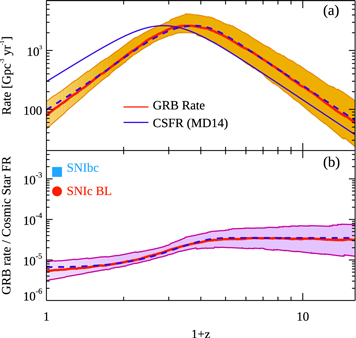
Figure 3. Top panel: GRB formation rate (red solid line) and its 1σ uncertainty (shaded region). The solid blue line shows the CSFR (Madau & Dickinson 2014). The dashed blue lines show the CSFR modified by a metallicity threshold 12+ (Appendix A.3). The blue model curves have been normalized to the peak value of the GRB formation rate. Bottom panel: GRB to CSFR ratio (the red solid line, with its 1σ uncertainty). The dashed curve, corresponding to the metallicity thresholds, is normalized to the red curve at z ∼ 3. The fractions of local supernovae of Type Ibc and Type Ic-BL are shown by the red circle and the cyan square, respectively (see Strolger et al. 2015; Perley et al. 2020).
Download figure:
Standard image High-resolution imageThe local LGRB formation rate is  Gpc−3 yr−1 (68% confidence interval). This is derived by normalizing the model population: we consider the ∼170 ± 13 bright GRBs with peak fluxes in the 15–150 keV energy range ≥2.6 ph cm2 s−1 detected by Swift/BAT over 8 yr. We assume for Swift/BAT an average duty cycle of 0.75 and a fully coded field of view of 1.4 sr. We have verified that our results are unchanged if we renormalize the population to the bright GRB sample detected by Fermi/GBM, namely 902 LGRBs with P(10–1000) ≥ 5 ph cm2 s−1, detected over 11.8 yr within its 8.8 sr field of view, also accounting for a 0.55 duty cycle. Since our population accounts for the random orientation of GRB jets in the sky, the derived local rate represents the intrinsic one.
We also performed the same analysis under the assumption of a Schechter luminosity function, and the results are reported in Appendix A.2. We find that the shape of the LGRB rate at low redshifts is unchanged (Figure 6). The Schechter scenario produces a slightly shallower decrease in the GRB formation rate at high redshifts. However, this is consistent with the CSFR, given the uncertainties on high-redshift measurements.
5. Discussion and Conclusions
The LGRB efficiency as a function of redshift, defined as the ratio between the GRB rate and the CSFR, is shown in Figure 3(b) by the solid red line. Its 1σ uncertainty (the shaded violet region in Figure 3) is computed by resampling the posterior distributions of the free parameters shown in Figure 2 105 times. For the CSFR, we have also considered the function of Madau & Dickinson (2014; the solid blue line in Figure 3(a)). In the local universe, this ratio is ∼5 ×10⁻⁵
M⊙
−1, and it increases by up to a factor of 10 at z ∼ 3. In Figure 3(b), we show with the blue and red symbols, respectively, the fraction of star formation leading to Type Ibc and Type Ic broad-line (BL) supernovae (Perley et al. 2020), assuming the core-collapse supernova rate derived by Strolger et al. (2015). We find that, in the local universe,  of Type Ic-BL supernovae produce a jet and the associated GRB event. This fraction increases with redshift up to ∼7% at z > 3.
The general trend of the GRB cosmic rate at low redshifts shows a decrease in the efficiency of GRBs being produced with decreasing redshift (Figure 3). This result argues against the claims for an increase in the LGRB efficiency toward lower redshifts (the so-called low-redshift excess—Yu et al. 2015; Petrosian et al. 2015; Tsvetkova et al. 2017; Lloyd-Ronning et al. 2019; but see also Pescalli et al. 2016; Le et al. 2020; Bryant et al. 2021) obtained through nonparametric methods. The low-redshift GRB uptick could be partially absorbed if the jet opening angle evolves with redshift (Lloyd-Ronning et al.2020).
The GRB efficiency with redshift evolution can be interpreted as being due to the increase in metallicity with cosmic time, which prevents a larger fraction of massive stars from producing GRBs (Yoon et al. 2006). In order to verify this possibility, we compute the fraction of cosmic star formation in galaxies with average metallicity below a given threshold, following the method of Robertson & Ellis (2012). We combine (Appendix A.3) the mass–metallicity relation and its redshift evolution (Maiolino et al. 2008) with the galaxy mass function (McLeod et al. 2021) and the galaxy main sequence (Tomczak et al. 2014). We find that a metallicity threshold  8.6, represented by the the dashed blue lines in Figure 3, accounts for the derived GRB efficiency evolution. The metallicity thresholds we derive are consistent with the observed GRB host galaxy metallicity (Vergani et al. 2015; Palmerio et al. 2019). To further verify this consistency, we have computed the stellar masses of galaxies with metallicities below the threshold value found, and compared them with the observed masses of a complete sample of GRB hosts (Vergani et al. 2015; Palmerio et al. 2019; the black symbols in the left panel of Figure 4). The maximum and average stellar masses (the green and blue curves in the left panel of Figure 4) are shown for
  8.6 by the dashed lines and they are consistent with the measured masses of the hosts and their redshift evolutions.
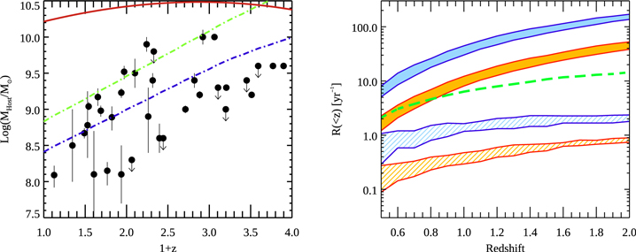
Figure 4. Left panel: mass–redshift distribution of LGRB host galaxies (black symbols; Vergani et al. 2015; Palmerio et al. 2019) compared to the average mass (blue curve) and maximum mass (green curve) corresponding to the metallicity threshold 12+ = 8.6. The red line shows the model assuming the GRB cosmic rate to be proportional to the CSFR. Right panel: Fermi (blue) and Swift (orange) cumulative detection rates (the shaded and dashed regions show the 1σ uncertainty) as a function of redshift. The dashed regions refer to off-axis events. The solid filled regions represent the total (on-axis and off-axis). The green dashed line shows the rate of the observed Swift GRBs with measured redshifts. This shows a reduction in the efficiency of the ground-based redshift measurement at z > 0.6.
Download figure:
Standard image High-resolution imagePrevious LGRB population studies (e.g., Firmani et al. 2004; Salvaterra et al. 2012; Palmerio & Daigne 2021) have showed that a pure density evolution (PDE) of the GRB formation rate, where the luminosity function is invariant with redshift, and a pure luminosity evolution (PLE), where the GRB formation rate is proportional to the CSFR, cannot be distinguished on the basis of the GRB peak flux and luminosity–redshift distributions. Our best model is intermediate between these two extreme scenarios, and, indeed, we find both the GRB formation rate evolving with redshift (Figure 3(b)) and a mild evolution of the characteristic GRB luminosity ∝(1 + z)0.64 (Table 1). We exclude at more than 5σ significance the extreme cases of PLE and PDE. Moreover, the PLE is also excluded by the host galaxy mass distribution (see the red line in Figure 4). The finding of the evolution of the LGRB characteristic luminosity ∝(1 + z)0.64 could hide the changes in some properties of the progenitors with redshift, possibly ruled by their metallicity (Yoon et al. 2006), which could induce a flattening of the initial mass function (Fryer et al. 2022).
This possibility can be tested by the increasing fraction of GRBs detected at high redshift, as envisaged by the next-generation missions optimized for this purpose (e.g., the Transient and High Energy Sky and Early Universe Surveyor, or THESEUS—Amati et al. 2021; or the Gamow Explorer—White et al. 2020).
Our population model, which implements the jet opening angles of GRBs and accounts for the observed properties as a function of the viewing angle, allows us to estimate the fraction of GRBs detected by Fermi/GBM and Swift/BAT that are observed off-axis, i.e., θv > θjet. The right panel of Figure 4 shows the expected cumulative rate as a function of redshift for Fermi/GBM (blue filled stripes) and Swift/BAT (orange filled stripes). The hatched curves show the detection rates of off-axis events according to our population. We estimate that ∼10% of the LGRBs detected by Fermi and Swift at z < 0.5, corresponding to a rate of 0.2–0.7 yr−1, should be observed off-axis. This fraction reduces to less than 3% at z < 2. In this work, we have adopted a uniform jet structure consistent with that suggested by study of the luminosity function of LGRBs (Pescalli et al. 2015). Therefore, our results should be considered as a conservative lower limit, since a universal structured jet should produce a larger fraction (e.g., Salafia et al. 2015) of detected off-axis events.
We acknowledge support from ASI-INAF agreement No. 2018-29-HH-0. We acknowledge PRIN-MIUR 2017 (grant 20179ZF5KS) and the "Figaro" premiale project (1.05.06.13). We thank S. Vergani, G. Ghisellini, and O. S. Salafia for constructive discussions. We acknowledge L. Amati and N. White, and the respective THESEUS and Gamow Explorer collaborations, for stimulating interactions over the past few years.
Appendix: Appendix Information
A.1. Consistency Checks
In order to verify the consistency of our model with the GRB samples detected by other instruments, we considered the full Swift/BAT and BeppoSAX/GRBM (Frontera et al. 2008) samples. We applied a peak flux cut, extracting 536 Swift/BAT GRBs with a 15–150 keV peak flux Fp ≥ 0.5 phot cm−2 s−1. Their observer-frame distributions are shown by the green asterisks in the top panels of Figure 5. For Beppo/SAX, we considered the 118 GRBs with a peak flux, integrated in the 40–700 keV energy range, Fp ≥ 10−6 erg cm−2 s−1. The Beppo/SAX distributions are shown by the pink asterisks in the bottom panels of Figure 5. The population model is shown by the solid histogram and shaded regions.
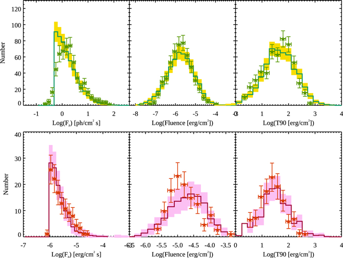
Figure 5. Consistency checks of the population model with the distributions of the peak flux, fluence, and duration of the GRBs detected by the Swift/BAT satellite (top row) and Beppo/SAX (bottom row). The Swift/BAT GRBs (green symbols) are obtained by selecting GRBs with a peak flux (15–150 keV) ≥ 0.5 ph cm−2 s−1, while the Beppo/SAX GRBs (pink symbols) are selected with a peak flux (40–700 keV) ≥ 10−6 erg cm−2 s−1. The model is shown by the solid lines, and its 1σ uncertainty (described as in Figure 1) by the solid filled histogram.
Download figure:
Standard image High-resolution imageA.2. Schechter Luminosity Function
We considered the possibility that the GRB luminosity function is described by a Schechter function (Schechter 1976), namely a power law with a high-luminosity exponential cutoff. This model has two free parameters, the slope of the power law α and the cutoff luminosity Lc
. We fix the minimum luminosity of this function to 1047 erg s−1. With this model, we can reproduce all the observational constraints described in Section 3. We obtain α = 1.15 ± 0.15 and  . The resulting GRB formation rate is shown in Figure 6 by the black line (and its 1σ uncertainty by the shaded region). For comparison, the CSFRs of Madau & Fragos (2017; blue line) and Madau & Dickinson (2014; green line) are shown. The modified CSFRs obtained with metallicity threshold cuts at 12+log(O/H) ≤ 8.6 and 8.4 are shown by the dashed and dotted–dashed lines, respectively. The GRB formation rate obtained under the Schechter assumption is consistent within its uncertainties with that obtained with a broken-power-law luminosity function, although it is slightly shallower at high redshifts.

Figure 6. GRB formation rate (black solid line) and its 1σ uncertainty (shaded region) obtained with the model described in Section 1, but assuming a Schechter luminosity function instead of Equation (2). The solid blue line shows the CSFR as derived by Madau & Fragos (2017) and the solid green line shows that obtained by Madau & Dickinson (2014). The dashed (dotted–dashed) lines are the CSFR functions modified by a metallicity threshold 12+ (8.4), respectively (Appendix A.3). The blue and green model curves have been normalized to the peak value of the GRB formation rate.
Download figure:
Standard image High-resolution image
A.3. Metallicity Bias Model
Following the formalism of Robertson & Ellis (2012), we estimate the fraction of star formation occurring in galaxies with metallicity below a given threshold as
where R⋆(M, z) is the star formation rate–stellar mass relation (M is the galaxy stellar mass in units of M⊙) and ϒ(M, z) is the galaxy mass function. Both these functions evolve with the redshift z. For R⋆(M, z), we assume the relation of Tomczak et al. (2014), and for ϒ(M, z) we consider the recently reported double Schechter galaxy mass function of McLeod et al. (2021). M⋆,th(z) is the maximum mass corresponding the the metallicity threshold,
obtained by inverting Equation (2) of Maiolino et al. (2008). The values of K(z) and M0(z) are interpolated from those reported in Table 5 of their paper. We also corrected (through the 0.04 term) for the different assumption of a Chabrier initial mass function in the host galaxy mass estimates shown in Figure 4.
Footnotes
- 4
The peak fluxes are reported in the Fermi online spectral catalog (https://heasarc.gsfc.nasa.gov/W3Browse/fermi/fermigbrst.html) and the 5B BATSE catalog (https://heasarc.gsfc.nasa.gov/W3Browse/cgro/bat5bgrbsp.html), as obtained by fitting the peak spectrum with the Band function.
- 5
- 6
For ease of comparison, this is rescaled to the value of the GRB formation rate at its peak.