


Abstract
The boundaries of solar coronal holes are difficult to uniquely define observationally but are sites of interest in part because the slow solar wind appears to originate there. The aim of this article is to explore the dynamics of interchange magnetic reconnection at different types of coronal hole boundaries—namely streamers and pseudostreamers—and their implications for the coronal structure. We describe synthetic observables derived from three-dimensional magnetohydrodynamic simulations of the atmosphere of the Sun in which coronal hole boundaries are disturbed by flows that mimic the solar supergranulation. Our analysis shows that interchange reconnection takes place much more readily at the pseudostreamer boundary of the coronal hole. As a result, the portion of the coronal hole boundary formed by the pseudostreamer remains much smoother, in contrast to the highly distorted helmet-streamer portion of the coronal hole boundary. Our results yield important new insights on coronal hole boundary regions, which are critical in coupling the corona to the heliosphere as the formation regions of the slow solar wind.
Export citation and abstract BibTeX RIS

Original content from this work may be used under the terms of the Creative Commons Attribution 4.0 licence. Any further distribution of this work must maintain attribution to the author(s) and the title of the work, journal citation and DOI.
1. Introduction
The solar wind streams outwards from the Sun to fill the heliosphere. It is typically observed to be either fast and steady or slow and unsteady, with these two types of wind also exhibiting differences in their composition (McComas et al. 1998; Abbo et al. 2016). The origin of the slow wind remains to be fully understood, although it appears to be associated with the boundaries of coronal holes (Abbo et al. 2010; Brooks et al. 2015; Macneil et al. 2019) (originally identified as dark regions in coronal emission where the plasma density is low; Cranmer 2009). These coronal hole boundaries are well correlated with the boundary between closed and open magnetic fluxes as determined from models. It is proposed, therefore, that interchange magnetic reconnection between open and closed flux is responsible for some of the properties of the slow wind (Fisk et al. 1998; Fisk 2003; Antiochos et al. 2011).
The boundaries of coronal holes are difficult to define uniquely in observations (Reiss et al. 2021). Indeed, they are rarely seen as a sharp transition in any emission line but rather often appear "fuzzy" or "ragged" (Kahler & Hudson 2002). Undoubtedly one factor contributing to this fuzziness is plasma and magnetic field dynamics. Therefore, in this paper, we use "coronal hole boundary" to mean the boundary between open and closed magnetic fluxes. Continual interchange reconnection can mix plasma from the dense (closed-field) region and the more tenuous (open-field) region, meaning that the plasma along reconnecting field lines never reaches a true thermodynamic equilibrium. The transition region between these two types of field lines, as defined by variation in plasma parameters, is expected to have an appreciable width due to continuous reconnection across a range of spatial scales (Karpen et al. 2012; Rappazzo et al. 2012; Pontin & Wyper 2015; Wyper et al. 2016). The apparent width of this layer may be further increased where photospheric flows lead to the corrugation of the coronal hole boundary so that the connectivity changes from open to closed multiple times along the line of sight.
2. Simulation Details
Here we build on previous simulations of interchange reconnection dynamics at the boundary between open and closed magnetic fluxes in the corona (Higginson et al. 2017a, 2017b; Aslanyan et al. 2021). We consider an isolated, midlatitude coronal hole bounded to the north by a pseudostreamer and to the south by a helmet streamer. A planar cut-through part of the simulation domain is shown in Figure 1, showing regions of open and closed magnetic field lines. The pseudostreamer is the small, red, dome-like structure in the top right of the solar disk, the helmet streamer of interest is the large red streamer on the right limb of the Sun, and the coronal hole of interest is indicated by the wedge of blue between the two. The initial magnetic field geometry and plasma parameters were taken directly from Wyper et al. (2021), whereupon the grid resolution was increased for this simulation.
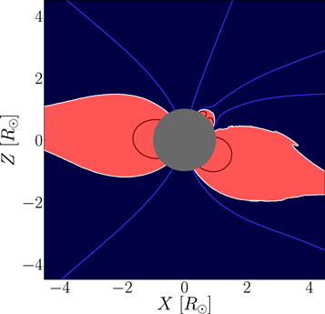
Figure 1. Vertical cut through the three-dimensional MHD simulation domain showing magnetic field structure. Outside the photosphere (gray), regions filled with open magnetic field lines are colored blue, closed regions colored red, and the border between them highlighted by the white line (not itself a field line). Sample field lines are indicated in blue and red respectively. The small isolated closed region in the top right is the pseudostreamer.
Download figure:
Standard image High-resolution imageThe time-dependent magnetic field structure in the solar corona was computed using the Adaptively Refined Magnetohydrodynamic Solver, as reported in DeVore (1991). This code solves the three-dimensional magnetohydrodynamic (MHD) equations with gravity, assuming an isothermal plasma with a temperature T = 1 MK. Consequently, while the magnetic field dynamics and effects such as reconnection are well resolved (due to the low numerical dissipation), the code does not produce a realistic coronal temperature and density profile. The simulations began with a static magnetic field equilibrium computed using the potential field source surface model from the photosphere to an outer boundary at 30 R⊙. The system was subsequently allowed to relax into a dynamic equilibrium including an outflowing wind. Following this relaxation phase, flows were applied on the photospheric boundary, leading to a dynamic evolution, as described in the following section.
At selected times in the MHD simulation, magnetic field lines have been integrated to build up a binary open/closed classification of a volume close to the photosphere. Here, a "closed" field line connects at both ends to the photosphere while an "open" field line connects the photosphere to the outer radial boundary of the domain. One way to visualize the geometry of the open and closed magnetic field lines that give rise to observations of coronal holes is to consider the last closed-flux surface—a separatrix in three dimensions demarcating the border between open and closed field lines. At the beginning of the simulation, this surface is shown in Figure 2(a), colored by the radius from the center of the Sun. The perspective is in the plane of Figure 1, looking at the midlatitude and northern polar coronal holes from the top-right corner; the white line there is a cut through the last closed-flux surface. The "true" magnetically defined coronal hole boundary is the line where the last closed-flux surface intersects the photosphere. Such a boundary is shown relative to synthetic EUV images (as described below) in Figures 2(b) and (c).
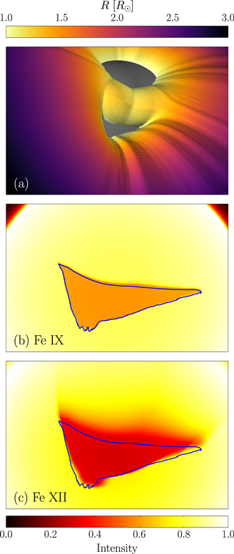
Figure 2. (a) Visualization of the last closed-flux surface around the Sun (gray sphere) in the vicinity of the midlatitude coronal hole. The viewing perspective is from approximately the top-right corner of Figure 1. Magnetic field lines inside the surface are closed, while any field line connected to the two visible coronal holes is open. Synthetic emission from atomic iron with charge states (b) Fe ix and (c) Fe xii at the beginning of the simulation. The lower end of the intensity scale is identically zero in all cases, while its upper end has been adjusted for each charge state. The images of synthetic emission are along the same axis but zoomed in relative to panel (a). The difference in intensity between the coronal hole and the surrounding regions arises due to the higher density and temperature of the plasma in the closed-field region. The blue lines indicate the coronal hole boundary, where the last closed-flux surface intersects the photosphere.
Download figure:
Standard image High-resolution imageWe postprocessed the resulting fully 3D MHD equilibrium with temperatures and densities obtained from the HYDRAD code (Bradshaw & Klimchuk 2011). HYDRAD is a self-consistent one-dimensional code that includes empirical coronal heating, thermal conduction, and radiative losses. Using this code, we computed two radially dependent temperature and density profiles that extend from the solar surface to the limit of the MHD domain using a representative coronal heating profile, as shown in Figure 3. In the first case, we imposed a flow-through boundary condition that resulted in a transonic wind solution, while in the second case we used a reflecting boundary condition that resulted in a near-static solution corresponding to the largest possible closed-loop solution for our model. Each of the two profiles contains a model chromosphere above which the temperature rises abruptly through the transition region while the density falls to coronal values. At every point in the 3D MHD simulation domain, we assigned a temperature and density based on the radius of that point from the first HYDRAD profile if the local magnetic field line was open and from the second profile if it was closed. This approach captures the generic difference in the plasma structure of a closed versus open flux tube but does not rigorously calculate the plasma structure of a fully dynamic 3D corona and wind, which, in any case, would be highly dependent on whatever assumptions are made for the coronal heating and solar wind acceleration mechanisms. Because we are not attempting to match some particular set of observations and are using only a generic model for the magnetic field and driving motions, our simple approach is sufficient to predict the qualitative observational difference between coronal holes and closed regions. Note that the closed-field profile is systematically hotter and denser, especially at larger heights.

Figure 3. Density and temperature obtained from the HYDRAD code with boundary conditions corresponding to open and closed field lines, respectively.
Download figure:
Standard image High-resolution imageThe temperature and density profiles are used to generate an image of line emission from selected ion species using the FOMO code (Van Doorsselaere et al. 2016). FOMO computes the emissivity of a selected ion at a given wavelength on a three-dimensional grid. The emissivity is obtained from the local temperature and density using the CHIANTI database (Landi et al. 2013) assuming the plasma is in thermal equilibrium. The line-of-sight emissivity  of coronal plasma is then integrated to build up images. We choose two charge states of iron that emit in the following EUV wavelengths: 17.1 nm (Fe ix) and 19.4 nm (Fe xii). These wavelengths would correspond to channels of the AIA instrument on board the Solar Dynamics Observatory if other sources of emission were considered negligible and the instrument response function was ignored. The emissivity in each of these wavelengths reaches a peak at varying heights above the photosphere due to the increasing temperature. Emission from open field lines is consistently lower due to the lower densities and temperatures, as described above.
Imaging of the different wavelengths allows the shape of the coronal hole above the photosphere to be determined, as shown at the beginning of the simulation in Figures 2(b) and (c). The view is along the same line of sight but zoomed in relative to the image of the last closed flux surface. The viewing angle is 30° above the ecliptic, which would be observable by the Solar Orbiter or by other spacecraft if an analogous coronal hole existed at the solar equator. The shape of the "true" coronal hole boundary is indicated by the blue lines. The Fe ix emission, which comes from just above the photosphere, closely matches the shape of the coronal hole boundary. However, the Fe xii emission from higher in the corona follows its shape less closely. The coronal hole appears to be enlarged to the north, where pseudostreamer field lines curve out of the field of view, and narrower in the south, where helmet-streamer field lines curve into the field of view. Line-of-sight effects and perspective clearly play important roles in determining the extent of this effect, which should be present in actual observations. The primary limitations of our conclusions are the simplified temperature and density models for plasma on closed and open field lines. Many effects are likely to be present in the real corona such as thermal nonequilibrium, time-dependent heating, and others not modeled in this work, which could well complicate the identification of coronal hole boundaries in observations.
3. Results
Following the relaxation, we have performed two separate simulations with photospheric flow patterns alternatively at the southern ("helmet-streamer drive") and northern ("pseudostreamer drive") coronal hole boundaries as described in detail in Aslanyan et al. (2022). We evolved our MHD model for a total of 10 hr while applying photospheric motions intended to mimic supergranulation. Specifically, a set of flows in the manner of vortices is imposed on the lower photospheric boundary. Each of these vortical flows lasts approximately 5.5 hr (partially overlapping in time with the others) with a diameter of ≳25 Mm. The time envelope is sinusoidal, with a maximum flow speed ∼10 km s−1. Overall, the vortices are made somewhat larger and much faster than realistic supergranules due to computational limitations. However, footpoints of field lines are moved by no more than a supergranular scale under the influence of each vortex, as is the case for real supergranules. Clearly, the driving employed is a simplified representation of true photospheric motions, as, for example, the driving at scales below supergranulation (unresolvable in the simulation) is ignored. However, what our boundary flows do reproduce, importantly, is the complex mixing that leads to the development of small-scale structures and is generically found in the analyses of observed photospheric motions (e.g., Yeates et al. 2012; Candelaresi et al. 2018; Chian et al. 2019). Such analyses additionally show that the diverging/converging part of the flow induces negligible complexity in the coronal field, justifying our choice of purely vortical motions (Yeates et al. 2012; Candelaresi et al. 2018). We emphasize that the detailed nature of the coronal hole boundary deformation may not exactly mimic any true solar evolution, but the driving contains the relevant characteristic properties to allow a physically relevant comparison between helmet-streamer and pseudostreamer boundary segments.
Temperature, density, and EUV emission are obtained by postprocessing the dynamic magnetic field structure at any selected time as described above.
In each of the two cases, the driving flows inject energy into the domain, deforming the magnetic field from the initial configuration. The stresses accumulate on the helmet-streamer and pseudostreamer separatrix surfaces, inducing interchange reconnection (as in Aslanyan et al. 2021). The last closed flux surface and EUV images in the two wavelengths of interest are shown at the end of both simulations in Figure 4, all from the same perspective. The location of the driving can be seen from the contortion of the low-emission region, most clearly from the Fe ix ions close to the photosphere. We find that the coronal hole boundary is visibly much more complicated in the case where the boundary of the helmet streamer has been driven due to differing interchange reconnection dynamics. One major cause of this disparity is the difference in length between the field lines within the pseudostreamer and helmet streamer. A given footpoint motion produces proportionately greater stress on the shorter pseudostreamer field lines, stimulating interchange reconnection more readily. We expect the overall deformation of the coronal hole boundary seen in these simulations to match observed levels of deformation on the Sun after several days when accounting for the faster flow speeds in our simulations.

Figure 4. Last closed-flux surface and synthetic emission in the vicinity of the coronal hole at the end of the simulations. The coronal hole boundary as defined by magnetic field connectivity is indicated by the blue lines. Photospheric driving flows have been imposed at the helmet streamer (left column) and pseudostreamer (right column). The height of the peak emission of the indicated charge states is ordered to increase going down the page. Note the greater complexity of the coronal hole boundary in the case of the driven southern boundary with the helmet streamer, compared to the northern pseudostreamer boundary.
Download figure:
Standard image High-resolution imageTesting these findings observationally from EUV images requires a robust analysis technique, which is ideally scale independent. One approach to analyze the geometric complexity of objects of arbitrary spatial dimension is the "box-counting" fractal dimension (Ott 2002), defined as

where the object occupies a number N(w) of boxes, each of width w. This metric has been applied to curves in two-dimensional space with a wide range of scales from microscopic defects to the borders of countries. For example, a straight line has a box-counting fractal dimension D = 1, while the well-known Koch snowflake of infinite length bounding a finite area has  . The first step to compute D is to extract the shape of the observed coronal hole boundary. In Figure 5(a), we show the apparent shape of the coronal hole extracted from the synthetic Fe ix emission at the end of the pseudostreamer drive simulation by means of simple intensity thresholding. More advanced methods have also been applied to EUV observations. If the image is divided into square boxes of size w, an algorithm can then count the number of boxes N(w) that lie over the coronal hole boundary. Boxes that satisfy this criterion for two values of w are shown in Figures 5(b) and (c). The fractal dimension D is then obtained from a linear regression as the negative slope of
  plotted against
  .
.
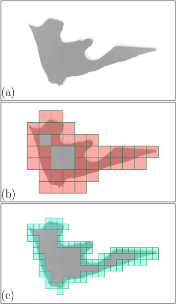
Figure 5. Illustrative method for computing the fractal dimension of a coronal hole using the box-counting method. (a) A binary map obtained from the synthetic image in Figure 4(d). The map is overlaid with square boxes of varying size w. The number of boxes that contain part of the boundary N(w) is counted, such as for (b) w = 8 and (c) w = 4. The fractal dimension is the negative slope of  against
  .
.
Download figure:
Standard image High-resolution imageTable 1 lists the box-counting fractal dimension D for all the synthetic coronal hole images shown above. The analysis quantitatively supports the intuitive assessment that the helmet-streamer-driven case is more complicated than the pseudostreamer-driven case, which in turn is more complicated than the coronal hole at the start of the simulations. The images of Fe xii emission have a systematically lower fractal dimension than the Fe ix because of the difficulty in identifying a sharp transition boundary in the former case, but the trend continues nonetheless. The box-counting method can be applied to open or piecewise curves. For a realistic coronal hole, driven everywhere on its perimeter and likely bounded by pseudostreamers and helmet streamers alike, the method can be applied to different parts of the border in turn. For practical purposes, there is a lower limit on w stemming from the resolution of an instrument or the size of pixels on a detector. To isolate the mechanism described presently from other processes not considered in this study, we propose comparing the average fractal dimension 〈D〉 of a statistically significant set of labeled coronal hole boundaries.
Table 1. Coronal Hole Fractal Dimension D for the Synthetic Images as Indicated
| Case | Figure | Fractal dimension |
|---|---|---|
| Start, Fe ix | 2(b) | 1.079 |
| PS-drive, Fe ix | 4(c) | 1.138 |
| HS-drive, Fe ix | 4(d) | 1.246 |
| Start, Fe xii | 2(c) | 1.035 |
| PS-drive, Fe xii | 4(e) | 1.096 |
| HS-drive, Fe xii | 4(f) | 1.178 |
Download table as: ASCIITypeset image
Another approach to quantify the differing complexity of the coronal hole in the two simulations, which may be more difficult to reproduce for observations, is to consider its perimeter at the photosphere. In order to avoid the "coastline paradox" (infinite boundary length for a finite area), we choose a single resolution for our analysis. The time history of the perimeter computed in this manner is shown in Figure 6. The total area of the coronal hole remains approximately constant—the supergranular motion deforms the boundary but does not force an expansion or contraction. A modest increase in the perimeter (by a factor of ∼1.2) is observed in the case where the pseudostreamer boundary is driven, with this increase saturating at around 20,000 s. By contrast, when the helmet-streamer boundary is driven, a systematic increase in the perimeter length is observed, which has still not saturated by the end of the simulation. An eventual saturation is expected only when the interchange reconnection balances the complexity being injected by the driving. We note that the factor by which the length increases in the two simulations is likely to be influenced by the magnetic Reynolds number, and so the relative increases rather than absolute increases are most noteworthy. We also note that time-dependent effects and varying field line lengths will further complicate the emission signatures as discussed in the first two sections of this article. Future studies should resolve these issues by augmenting the magnetohydrodynamic model with equations of thermodynamics, as was demonstrated in, e.g., Lionello et al. (2009) or van der Holst et al. (2014), though the step up in computational complexity and cost is substantial.

Figure 6. Perimeter of the coronal hole throughout simulations. The boundary is driven at the helmet streamer and pseudostreamer as indicated. The perimeter has been calculated at the photosphere and normalized to its value at the beginning of the simulation.
Download figure:
Standard image High-resolution image
4. Conclusion
This work predicts a marked difference between the parts of coronal hole boundaries formed by streamers and by pseudostreamers on the basis of different interchange reconnection dynamics. This result provides important new insights into these coronal hole boundary regions, namely, that the complexity of the coronal hole boundary along driven helmet-streamer structures appears greater than the complexity of the boundary along pseudostreamer structures, as evidenced by both coronal hole boundary segment length and fractal dimension. These regions are critical in coupling the corona to the heliosphere as the formation regions of the slow solar wind. We believe that this effect should be generic and, as illustrated in the synthetic images presented here, readily observable. Some care should be taken to distinguish this effect from variations below the supergranular scale. While some indication of this effect has been documented (Kahler & Hudson 2002), a necessary next step is to search for such systematic variations in high-resolution EUV/X-ray observations.
This work was performed using resources provided by the Cambridge Service for Data Driven Discovery (CSD3) operated by the University of Cambridge Research Computing Service, provided by Dell EMC and Intel using Tier-2 funding from the Engineering and Physical Sciences Research Council (capital grant EP/P020259/1), and DiRAC funding from the Science and Technology Facilities Council. V.A. is supported by the Science and Technology Facilities Council, grant number ST/S000267. R.B.S. is supported by the Office of Naval Research 6.1 basic research program. A.K.H. and R.B.S. were in part supported by the NASA Parker Solar Probe WISPR program. S.K.A. was supported by the NASA LWS Program. The authors would like to thank Emily Mason for fruitful discussions about coronal hole perimeters.