


Abstract
Quasars (QSOs) are extremely luminous active galactic nuclei currently observed up to redshift z = 7.642. As such, they have the potential to be the next rung of the cosmic distance ladder beyond Type Ia supernovae, if they can reliably be used as cosmological probes. The main issue in adopting QSOs as standard candles (similarly to gamma-ray bursts) is the large intrinsic scatter in the relations between their observed properties. This could be overcome by finding correlations among their observables that are intrinsic to the physics of QSOs and not artifacts of selection biases and/or redshift evolution. The reliability of these correlations should be verified through well-established statistical tests. The correlation between the ultraviolet and X-ray fluxes developed by Risaliti & Lusso is one of the most promising relations. We apply a statistical method to correct this relation for redshift evolution and selection biases. Remarkably, we recover the the same parameters of the slope and the normalization as Risaliti & Lusso. Our results establish the reliability of this relation, which is intrinsic to the QSO properties and not merely an effect of selection biases or redshift evolution. Hence, the possibility to standardize QSOs as cosmological candles, thereby extending the Hubble diagram up to z = 7.54.
Export citation and abstract BibTeX RIS

Original content from this work may be used under the terms of the Creative Commons Attribution 4.0 licence. Any further distribution of this work must maintain attribution to the author(s) and the title of the work, journal citation and DOI.
1. Introduction
The quest for standard candles at high redshifts is still open, with the aim of extending the Hubble diagram out beyond the epoch of reionization. Since the discovery of gamma-ray bursts (GRBs) as extragalactic sources, hosts of high-redshift sources have been identified, including GRB 090423 (Tanvir et al. 2009) and GRB 090429B (Cucchiara et al. 2011). Recently, quasars, or quasi-stellar objects (QSOs), have also been observed at high redshifts, reaching up to z = 7.54 (Bañados et al. 2018) and z = 7.64 (Wang et al. 2021). One of the biggest challenges for the use of these objects as standardizable candles is the large scatter in the relations among their intrinsic properties. Since 2002, many authors in the GRB community have investigated the possibility of using GRB relations as cosmological probes (Dainotti et al. 2008, 2010, 2011a, 2011b, 2013a, 2013b, 2015a, 2015b, 2016, 2017, 2018, 2020a, 2020b, 2021a, 2021c, 2021d, 2021e; Cardone et al. 2010; Dainotti & Del Vecchio 2017; Postnikov et al. 2014; Dainotti & Amati 2018; Srinivasaragavan et al. 2020; Cao et al. 2022a, 2022b). The search for high-redshift standard candles has been boosted by the Hubble tension, a 4σ–6σ discrepancy between the direct measurements of local H0 and H0 inferred from cosmological models, most notably the value reported by the Planck observation within the ΛCDM model. Additional high-z standardized probes beyond Type Ia supernovae (SNe Ia), such as GRBs and QSOs, could be instrumental in shedding light on this problem (Capozziello et al. 2020a, 2020b; Dainotti et al. 2021b, 2022a; Bargiacchi et al. 2021; Moresco et al. 2022).
QSOs are extremely luminous active galactic nuclei (AGNs). Their emission cannot be explained by standard stellar processes and requires a different kind of mechanism, e.g., mass accretion onto the central supermassive black hole (see, e.g., Srianand & Gopal-Krishna 1998; Horowitz & Teukolsky 1999; Netzer 2013; Kroupa et al. 2020). This mechanism can indeed explain the observed properties of QSO emission, especially (as far as we are concerned) the UV and X-ray emissions. The accretion disk emits photons in the UV band, which are then processed through the inverse Compton effect by an external plasma of relativistic electrons, giving rise to X-ray emission. This physical explanation, while plausible, fails to account for the stability of the X-ray emission. Ultimately, one needs an efficient energy transfer between the accretion disk and the external relativistic "corona" to explain such stable emission. The physical origin of this link between the two AGN regions is not known yet. However, some models have been proposed (see, e.g., Lusso & Risaliti 2017) yielding relations that have been confirmed by the empirical correlation between UV and X-ray QSO luminosities. One of the most remarkable QSO correlations proposed so far is the so-called Risaliti–Lusso relationship among the fluxes in the UV and X-ray bands, based on the nonlinear relation between their UV and X-ray luminosities (Tananbaum et al. 1979; Avni & Tananbaum 1982, 1986; Kriss & Canizares 1985; Vignali et al. 2003; Steffen et al. 2006; Just et al. 2007; Lusso et al. 2010; Lusso & Risaliti 2016; Bisogni et al. 2021). The relation is extremely powerful because, if true, it allows one to standardize QSOs across a wide range of luminosities. This relation has been applied as a cosmological tool, and more generally the QSOs community is currently investigating the application of QSOs in other methods as cosmological tools and the possible problems associated with them (e.g., Khadka et al. 2021a, 2021b). In terms of luminosities, the Risaliti–Lusso relation may be expressed as 12

where β and γ are (constant) fitting parameters and

where UV and X refer to 2500 Å and 2 keV, respectively.
We here point out that the formula is written in a way for which the LX is derived by LUV since the UV photons are emitted by the accretion disk that represent the "seeds" for the X-ray emission of the corona through inverse Compton scattering. Indeed, if one can turn off the disk the corona will immediately follow, but the opposite is not true. If one can turn off the corona, the disk will still emit its luminosity regardless.
We note that luminosities are obtained applying a K-correction. The K-correction is defined as 1/(1 + z)1−α where α is the spectral index of the sources and it is assumed to be 1 for the sources, leading to K = 1, so hereafter the K-correction has been omitted following Lusso et al. (2020). In Equation (1), once we substitute Equation (2), the dependence on the luminosity distance DL becomes evident. This relation has been confirmed using various samples of QSOs, but with a very large intrinsic dispersion, hereafter denoted with δ; δ ∼ 0.35/0.40 dex in logarithmic units (e.g., Lusso et al. 2010). Only recently has it been pointed out that this dispersion has mainly an observational and non-intrinsic origin (Lusso & Risaliti 2016). This finding has allowed the intrinsic scatter to be reduced to δ ∼ 0.2 dex and has rendered this relation suitable for cosmological analyses, turning QSOs into reliable cosmological tools. We refer to Lusso & Risaliti (2016), Risaliti & Lusso (2019), and Lusso et al. (2020) for a more detailed description of the physics of this relation and its cosmological use.
This method has been developed only very recently and still needs to be tested and checked against different possible issues mainly related to selection biases, the dependence of the relation on the black hole mass and accretion rate in the AGN, and redshift evolution; thus further tests are needed to probe its reliability. Some of its issues are highlighted in Yang et al. (2020) and Khadka & Ratra (2021, 2022).
To fully cast light on the intrinsic nature of this relation, here we perform for the first time in the literature its correction for selection biases and the effects of redshift evolution with reliable statistical methods. If such biases were present, they could invalidate its reliability from a physical point of view and as a cosmological application. More precisely, if the correlation was merely induced by selection biases and redshift evolution, the slope of the correlation after correction for the biases and the evolution should have been compatible with a slope of zero within 5σ. This is not the case, and as we demonstrate here, the slope of the Risaliti–Lusso relation is not compatible with zero even at the 52.9σ level after we apply the corrections. In this paper, we explore the standardization of QSOs in view of future cosmological applications. In Section 2, we discuss in detail the QSO sample we use. Section 3 is devoted to the statistical analysis and the discussion of both selection biases and redshift evolution. In Section 4, we consider the Risaliti–Lusso correlation with the aim of verifying its intrinsic nature. In Section 5 we summarize our results and discuss future perspectives.
2. The Sample
We use the most up-to-date sample of Risaliti–Lusso QSOs (Lusso et al. 2020). This is composed of 2421 sources in the redshift range z = 0.009–7.54. These sources have been carefully selected for cosmological studies addressing possible observational issues, such as dust reddening, host-galaxy contamination, X-ray absorption, and Eddington bias, as detailed in Lusso et al. (2020). In particular, all QSOs with a spectral energy distribution (SED) that shows reddening in the UV and significant host-galaxy contamination in the near-infrared, are removed, leaving only sources with extinction E(B − V) ≤ 0.1. This requirement is fulfilled by selecting only the sources that satisfy  , where Γ1,UV and Γ2,UV are the slopes of a log(ν)–log(νLν
) power law in the rest frame 0.3–1 μm and 1450–3000 Å ranges respectively, and ν and Lν
denote the frequency and the luminosity per unit of frequency. The specific values Γ1,UV = 0.82 and Γ2,UV = 0.4 refer to a SED with zero extinction. In addition, X-ray observations where photon indices (ΓX) are peculiar or indicative of X-ray absorption are excluded by requiring ΓX + ΔΓX ≥ 1.7 and ΓX ≤ 2.8 if z < 4 and ΓX ≥ 1.7 if z ≥ 4, where ΔΓX is the uncertainty on the photon index. Finally, the remaining observations are filtered to correct for the Eddington bias.
, where Γ1,UV and Γ2,UV are the slopes of a log(ν)–log(νLν
) power law in the rest frame 0.3–1 μm and 1450–3000 Å ranges respectively, and ν and Lν
denote the frequency and the luminosity per unit of frequency. The specific values Γ1,UV = 0.82 and Γ2,UV = 0.4 refer to a SED with zero extinction. In addition, X-ray observations where photon indices (ΓX) are peculiar or indicative of X-ray absorption are excluded by requiring ΓX + ΔΓX ≥ 1.7 and ΓX ≤ 2.8 if z < 4 and ΓX ≥ 1.7 if z ≥ 4, where ΔΓX is the uncertainty on the photon index. Finally, the remaining observations are filtered to correct for the Eddington bias.
The final cleaned sample is hence composed only of sources satisfying  , where
  stands for a filtering threshold value and
  is the X-ray flux expected from the observed UV flux assuming the Risaliti–Lusso FX–FUV relation with fixed γ and β within the flat ΛCDM model with ΩM
= 0.3 and H0 = 70 km s−1 Mpc−1. Flim is the flux limit of the specific observation estimated from the catalog. The value of
is the X-ray flux expected from the observed UV flux assuming the Risaliti–Lusso FX–FUV relation with fixed γ and β within the flat ΛCDM model with ΩM
= 0.3 and H0 = 70 km s−1 Mpc−1. Flim is the flux limit of the specific observation estimated from the catalog. The value of  required in this filter is 0.9 for the Sloan Digital Sky Survey (SDSS) SDSS-4XMM and XXL subsamples and 0.5 for the SDSS-Chandra.
For any QSO, all the multiple X-ray observations that survive the filters above are finally averaged to minimize the effects of X-ray variability. The cleaned sample used in this work is the product of all these selection criteria.
3. Statistical Analysis to Overcome Selection Biases and Redshift Evolution
We apply the statistical method of Efron & Petrosian (1992, EP), which is able to correct for selection biases and redshift evolution, thereby uncovering intrinsic correlations in extragalactic objects (such as QSOs and GRBs). The reliability of this procedure has already been demonstrated via Monte Carlo simulations for GRBs (Dainotti et al. 2013b). We detail the method in the Appendix, while here we only summarize the crucial points required by the present work.
Following the approach in Dainotti et al. (2013a, 2015a, 2017, 2021a), we can correct for the evolution and obtain the local variables, in our case the luminosities. These new variables denoted with ' are the so-called "de-evolved variables," since the evolution has been removed. Such a removal may be achieved using the function g(z) = (1 + z)k
where the k parameter mimics the evolution with redshift and the new, de-evolved luminosities  are obtained from the original L via
  . The functional form for g(z) can be a simple power law (Dainotti et al. 2013a, 2017), similarly to this one, or a more complex function such as
  shown in Singal et al. (2011), where Z = 1 + z, which allows for a more rapid evolution up to redshift zcrit than the less rapid one at higher redshifts. This is a good fit for a QSO data set based on SDSS with many QSOs at z > 3 (Singal et al. 2013, 2016, 2019). In this work, we use the latter form with a fiducial critical redshift zcrit = 3.7, which is the most suitable value given the high-redshift distribution of the QSOs determined in Singal et al. (2013), but we also check our results against the specific functional form, allowing also for a simple power law. Interestingly, the same g(z) was shown to reproduce the observed luminosity function of AGNs (Singal et al. 2013).
Here, we detail our results of the EP method for the studied parameters for the whole sample of 2421 QSOs considering the evolutionary form with zcrit = 3.7. The EP method takes into account both possible biases from incomplete data and redshift evolution of observables by using an adaptation of the Kendall τ statistic (see Dainotti et al. 2013b and Section 7 of Dainotti et al. 2015a for a more detailed description). This test allows determination of the correlation between two generic variables (xi , yi ) and the best-fit values of parameters describing their correlation function by defining the parameter τ as
where  is the rank of yi
in a set associated with it, and
is the rank of yi
in a set associated with it, and  and
and  are its expectation value and variance, respectively. For untruncated data the associated set includes all of the data with xj
< xi
. In our case in which we have truncation, the associated set for zi
contains all QSOs with
are its expectation value and variance, respectively. For untruncated data the associated set includes all of the data with xj
< xi
. In our case in which we have truncation, the associated set for zi
contains all QSOs with  and zj
≤ zi
. Here j and i denote objects of the associated set and the overall QSO sample, respectively, and
and zj
≤ zi
. Here j and i denote objects of the associated set and the overall QSO sample, respectively, and  is the minimum luminosity that would still allow us to detect an object at a given zi
. More specifically,
is the minimum luminosity that would still allow us to detect an object at a given zi
. More specifically,  is computed for each data point considering the position of the data in samples including all the objects that can be detected for particular observational limits; see Efron & Petrosian (1992) for further details. If two variables are independent,
  should be distributed continuously between 0 and 1 with
  and
and  . Independence is rejected at the n
σ level if ∣τ∣ > n. With this statistic, we find the parameterization that best describes the evolution. For the present study, we are interested in analyzing the redshift evolution of QSO UV and X-ray luminosities to test their degree of correlation in the
. Independence is rejected at the n
σ level if ∣τ∣ > n. With this statistic, we find the parameterization that best describes the evolution. For the present study, we are interested in analyzing the redshift evolution of QSO UV and X-ray luminosities to test their degree of correlation in the  and
and  spaces. To eliminate the dependence of the redshift on our variables of interest, we require τ(k) = 0, which implies the de-evolved luminosities are statistically independent of the redshift. The value of k corresponding to τ = 0 gives us the exact redshift evolution of LUV and LX within 1σ, determined from ∣τ∣ ≤ 1, according to our chosen functional form for g(z). Here, we detail the computations to derive the evolutionary coefficients and follow the same procedure for both LUV and LX.
From the measured flux we compute the luminosity for each QSO assuming a flat ΛCDM model with ΩM = 0.3 at the current time and H0 = 70 km s−1 Mpc−1. Note that in this investigation it is shown that the values of the evolutionary parameters for QSOs do not evolve significantly with the cosmological parameters such as ΩM and H0. Thus, we can safely use this test with any given cosmological model and we explicitly use this test later in Section 3.1. There is also an ongoing discussion on the validity of the Risaliti–Lusso relation and its effectiveness beyond z ∼ 1.5 due to discrepancies between QSOs and SNe Ia; for example, see Yang et al. (2020) and Khadka & Ratra (2021, 2022). However, this discussion is beyond the scope of the current paper.
We also compute the flux limit Flim and the corresponding luminosity  . According to Dainotti et al. (2013a, 2015a, 2017), Levine et al. (2022), and Dainotti et al. (2022b), the samples used to derive the evolutionary effects should not be less than 90% of the original ones and the population of X-rays and UV should resemble as far as possible the overall distribution. To this end, conservative choices regarding the limiting values are needed.
Specifically, we have chosen  for the UV and
  for the X-rays, which respectively guarantee samples of 2362 (97.6%) and 2379 (98.3%) QSOs. We have also verified through the means of the Kolmogorov–Smirnov (KS) test that the full and the cut samples in both X-rays and UV come from the same parent population. Indeed, the probability of the null hypothesis that the two samples are drawn from the same distribution cannot be rejected at p = 0.47 for the UV and p = 0.85 for X-rays.
The limiting values for LUV and LX corresponding to these values of Flim are shown with a black continuous line in the left and right panels of Figure 1, respectively, over the whole set of data points represented by red circles. We then apply the τ test to the data sets trimmed with values of the fluxes mentioned above and obtain the trend for τ(k) shown in the left and right panels of Figure 2 for the UV and X-rays, respectively. As already explained, τ = 0 and ∣τ∣ ≤ 1 provide us with the best-fit value and the associated 1σ error for the evolutionary parameter k. For the UV and X-rays we obtain k = 4.36 ± 0.08 and k = 3.36 ± 0.07, respectively. It is remarkable that the evolutionary function of the UV in our sample is compatible within 2.4σ with the optical evolutionary coefficient kopt obtained in Singal et al. (2013), where the same form of g(z) is used. In their paper they found kopt = 3.0 ± 0.5 and corrected the luminosity function with the central value. Thus, the new luminosity function can be representative of the observed luminosity function, but it will be constructed with the local luminosities (de-evolved luminosities), and thus they will be rescaled by the g(z) functions. Indeed, similarly to Singal et al. (2013), we expect that the results of our luminosity function are in agreement with the ones in the literature.
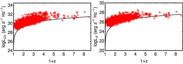
Figure 1. Redshift evolution of LUV (left panel) and LX (right panel) in units of erg s−1 Hz−1 for the whole QSO sample (red circles). The black line in both panels shows the limiting luminosity chosen according to the prescription described in Section 3.
Download figure:
Standard image High-resolution image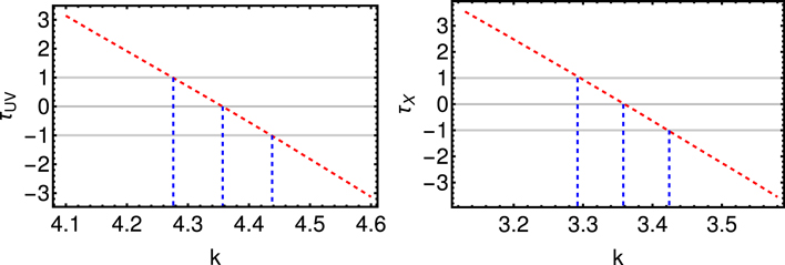
Figure 2. τ(k) function (dashed red line) for both the UV (left panel) and X-ray (right panel) analyses. The point τ = 0 gives us the k parameter for the redshift evolution of LUV and LX, while ∣τ∣ ≤ 1 (gray lines) is the 1σ uncertainty on it (dashed blue lines).
Download figure:
Standard image High-resolution imageHowever, we note that if a different method regarding the choice of the limiting luminosity is applied, the evolutionary functions are smaller (see Singal et al. 2022). The method detailed in Singal et al. (2022) takes into consideration a different limit for each source as  where the ratio of an object's j's indicates the significance σj
relative to its minimum significance
where the ratio of an object's j's indicates the significance σj
relative to its minimum significance  . This ratio is used to calculate the minimum X-ray flux for each source. In addition, we may note that in Singal et al. (2022) the K-correction has been applied to each source, while in our case the K-correction is assumed to be 1. Another major difference is that the sample used in the case of Singal et al. (2022) is taken from the SDSS DR7 (Schneider et al. 2010), whereas in our case we use a sample of 2421 sources from the newest release SDSS DR14 (Pâris et al. 2018). It is definitely interesting to consider this more complex approach with the flux limits in a forthcoming paper.
We have performed an additional test to legitimate our choice for Flim and prove that the evolutionary coefficients depend only weakly on these choices. In both X-ray and UV bands, we compute the evolutionary coefficient k for different limiting values Flim. Specifically, we started with a value of Flim that preserves the original sample and then analyzed a range of values for Flim. If we span 0.5 magnitude in the UV starting from  and in X-rays starting from
  we obtain a compatibility within 1σ. Even if we span one order of magnitude starting from the same Flim values in fluxes both in UV and in X-rays, the results for the evolutionary coefficient remain compatible within 2σ. This analysis proves that the results for the evolutionary coefficients do not depend on the specific choice of Flim for a wide range of their values.
Inserting our values of k in g(z), we then compute the new de-evolved luminosities, denoted with ', and the associated uncertainties for the whole original QSO sample. The comparison between these quantities and the initial ones is shown in Figure 3 in the ( ,
,  ) plane. Compared to the initial ones, the computed luminosities span a smaller region of the (
 ,
,  ) plane and show a slightly greater dispersion (δ ∼ 0.22 against δ ∼ 0.21, as evaluated in Section 4). This fact is expected because the g(z) function, once the best-fit values for k are used, yields a greater correction (i.e., lower de-evolved values) for higher luminosities. In addition, we have accounted for the error on the determination of k by propagating the errors on the g(z) function. This naturally increases the associated uncertainties on the luminosities. The correction for g(z) affects the spread of the luminosities, and hence the dispersion of the correlation, which is consequently larger. To summarize, the dispersion increases due to the larger spread of the luminosities and it is minimally affected by the error propagation due to g(z). In other words, the dispersion yielded by the function g(z) is larger than the contribution given by the additional errors due to g(z). Larger errors on the variables may reduce the dispersion, but in this case not by enough to balance the increase in the dispersion due to the function g(z).
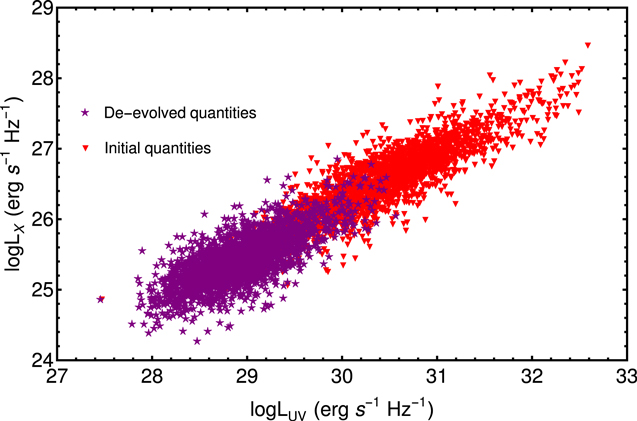
Figure 3. Comparison between initial (red) and de-evolved (purple) quantities in the ( ,
,  ) plane.
Download figure:
Standard image High-resolution imageWe also would like to point out that in a very recent paper (Dainotti et al. 2021d) it has been shown that this method is reliable regardless of the choice of the limiting values for several sample sizes for short GRBs (samples of 56, 34, and 32 GRBs). Thus, the discussion of Bryant et al. (2021) on the EP method and its applicability are not a concern given the approach and the reliability of the results in Dainotti et al. (2021d).
3.1. Impact of Cosmology on the g(z) Function
In order to compute the evolutionary parameter, k, for the luminosities one has to assume initial fiducial values of cosmological parameters. This could possibly lead to a circularity problem in cosmological measurements. We investigate the relation between the evolutionary parameter k and cosmology by repeating the evaluation of k following the same procedure over a set of 50 ΩM
values ranging from 0 up to 1. Results of this computation are shown in Figure 4. We note here that there is no change in the value of k when H0 is varied. This happens because of the relation between H0, the luminosity, and redshift. The Hubble constant is responsible only for an overall scaling of the distribution of the luminosities according to Equation (2). This does not change the number of associated sets for each redshift since both the luminosities and the limiting luminosities are scaled in the same way through the distance luminosity. Thus, there is no impact of H0 on k. The behavior of the k parameter as a function of ΩM
is not negligible in a wide range of investigated values, but its values remain compatible within 1σ for ΩM
= 0.3 for the sets of ΩM
∈ (0.20, 0.45) and ΩM
∈ (0.22, 0.41) for cases of  and
and  respectively. The 1σ, 2σ, and 3σ ranges are shown in red, orange, and green. The black line indicates the value of k for ΩM
= 0.3, which is our reference value given that we correct the Risaliti–Lusso relation with a g(z) based on ΩM
= 0.3. These ranges of values exceed the values of the most up-to-date cosmological measurements of ΩM
with SNe Ia (ΩM
= 0.298 ± 0.022, Scolnic et al. 2018) within error bars. Thus, we do not expect this effect to have a significant impact on cosmological constraints. We note that this study is important for any probe and it will be included in future analysis when QSOs are applied as cosmological probes. This method is very general and it can also be applied for any astrophysical sources observed at cosmological redshifts.
respectively. The 1σ, 2σ, and 3σ ranges are shown in red, orange, and green. The black line indicates the value of k for ΩM
= 0.3, which is our reference value given that we correct the Risaliti–Lusso relation with a g(z) based on ΩM
= 0.3. These ranges of values exceed the values of the most up-to-date cosmological measurements of ΩM
with SNe Ia (ΩM
= 0.298 ± 0.022, Scolnic et al. 2018) within error bars. Thus, we do not expect this effect to have a significant impact on cosmological constraints. We note that this study is important for any probe and it will be included in future analysis when QSOs are applied as cosmological probes. This method is very general and it can also be applied for any astrophysical sources observed at cosmological redshifts.
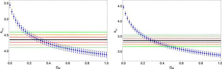
Figure 4. The dependence on the evolutionary parameter k for the LUV (left panel) and LX (right panel) luminosities on ΩM . The 1σ, 2σ, and 3σ ranges of the values of k are shown in red, orange, and green, respectively. The black line indicates the value of k for ΩM = 0.3 indicated in the text.
Download figure:
Standard image High-resolution image4. The Intrinsic logLX –logLUV Correlation
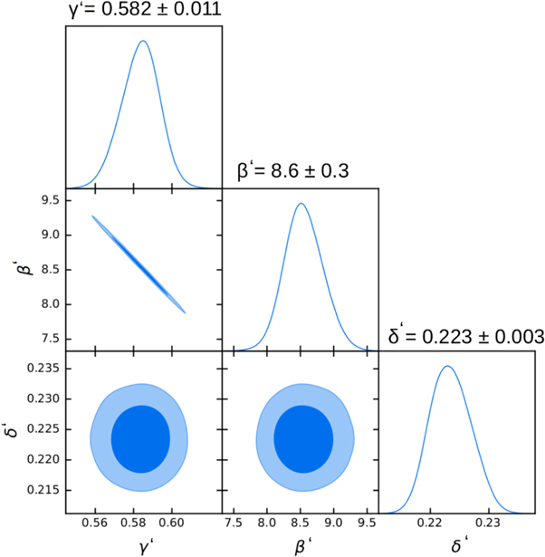
Having overcome the impact of selection biases and redshift evolution, we can now test whether the UV–X Risaliti–Lusso relation still holds between the de-evolved luminosities we computed. We compute the fitting parameters through a Bayesian technique, the D'Agostini method (D'Agostini 2005), to check whether the new de-evolved parameters—of the normalization, β', and the slope,  —are consistent within 1σ with the parameters not corrected for evolution, β and γ. We additionally use the Python package emcee (Foreman-Mackey et al. 2013) to further verify our results. These methods have the advantage of accounting for both error bars on x and y axes and an intrinsic dispersion δ. The likelihood used in the D'Agostini procedure is the following:
where σ(logLUV, i ) and σ(logLX, i ) are the uncertainties on the UV and X-ray fluxes, respectively.
The D'Agostini methods or similar ones are the most suitable because in our case we expect an intrinsic scatter in the UV–X relation and the error bars on both variables are not negligible. These two fitting techniques give completely consistent results within 1σ. Assuming a linear model of the form logL'X = γ' × logL'UV + β' with intrinsic dispersion δ, the resulting best-fit values for the free parameters and their associated 1σ uncertainties from the D'Agostini fit method are: γ' = 0.582 ± 0.011, β' = 8.6 ± 0.3, and δ = 0.223 ± 0.003. We show the corner plot corresponding to these values in Figure 5, where the covariance between  and
and  is just a mere effect of the fact that we perform the fit without normalizing the variables.
Figure 5. Results from the D'Agostini fit method assuming a linear model  for the de-evolved luminosities with intrinsic dispersion
  .
.
Download figure:
Standard image High-resolution image
Given our results, we have proven that the correlation is intrinsic to the physics of QSOs and not an artifact of selection biases and/or redshift evolution and that it can be used to turn QSOs into reliable cosmological probes. Remarkably, evolutionary parameters derived from the simple power law or the more complex function lead to the same results for the intrinsic slope of the correlation. While the simple power law g(z) = (1 + z)k
yields significantly different values for k in the UV and X-ray analyses, with discrepancies of 4.4σ and 5.3σ respectively, it leads to values for  ,
,  , and
, and  parameters consistent within 1σ with the values obtained from our other evolution function, as detailed in Table 1. Thus, we have shown that the relation is reliable against the specific choice of g(z) in the EP method. Therefore, any approach that involves the use of this correlation to derive cosmological parameters should take into account the evolutionary function for the luminosities, otherwise we could possibly see a trend of varying β and γ due to the fact that the evolution has not been removed.
Table 1. Best-fit Values and 1σ Uncertainties of  ,
,  , and
, and  Assuming Two Different Functional Forms for g(z)
| g(z) |

| β' |

|
|---|---|---|---|
| (Zk × 3.7k )/(Zk + 3.7k ) | 0.582 ± 0.011 | 8.6 ± 0.3 | 0.223 ± 0.003 |
| Zk | 0.578 ± 0.010 | 8.8 ± 0.3 | 0.223 ± 0.004 |
Note. For the sake of clarity, Z = 1 + z, as in the main text.
Download table as: ASCIITypeset image
To test the reliability of our results we check whether our fitting model assumes the scatter about the line to be Gaussian. We perform this test with both Anderson–Darling and Shapiro–Wilk normality tests on the whole QSO sample, but we do not recover a normal distribution. On the other hand, we do recover it if we apply a 3σ clipping on the sample while fitting the linear relation. This procedure removes iteratively the outliers from the fitting at a chosen value of σ from the fitting itself. In our case, we choose 3σ. Specifically, the sigma-clipping procedure removes only 1.2% of sources and remarkably does not change the best-fit values for the slope and the normalization, while it removes possible outliers. This procedure, which is an iterative method, has been previously reliably applied to this relation by Bargiacchi et al. (2021) and is commonly used when using QSOs for cosmological applications. Applying the two normality tests on this new cut sample, we recover a Gaussian distribution as we get pvalue = 0.18 from the Shapiro test and the result from the Anderson test that the null hypothesis that the sample comes from a normal distribution cannot be rejected at more than 15% significance level.
The best-fit values of γ' and δ' completely agree with the most recent ones reported in Lusso et al. (2020), which are obtained with a different approach in which de-evolved observables are not taken into account. Indeed, in that work, the FX–FUV relation is fitted in redshift bins so narrow that the spread in luminosity distance can be neglected compared to the intrinsic dispersion of the relation, and thus fluxes can be considered as proxies for luminosities. In this way, Lusso et al. (2020) establish the non-evolution of the slope γ with the redshift and find γ = 0.586 ± 0.061 and δ = 0.21 ± 0.06 with a simple forward fitting method. We stress that the method adopted here is completely nonparametric. To summarize, we show that  , since it has no statistically meaningful change compared to γ, undergoes no evolution, which is consistent with what is shown in Figure 8 of Lusso et al. (2020).
In the Lusso et al. (2020) analysis, the intercept fitted is not β itself, but a combination of β, γ, and the luminosity distance, so we cannot make an immediate comparison. Nevertheless, our value of β' after the correction for evolution is exactly the one expected from the literature (i.e., β ∼ 8.5) and the latest works on QSOs as standardizable candles (see, e.g., Risaliti & Lusso 2019; Lusso et al. 2020; Bisogni et al. 2021). These results establish that the Risaliti–Lusso relation is intrinsic to the physical processes in QSOs and is not a consequence of possible selection biases and redshift evolution, because it does not change once we have removed them. Other works have investigated several sources of selection bias due to the change in the viewing angle (Prince et al. 2021), but in a subsequent paper no such trend was found in the data (Prince et al. 2022). This supports the argument for no evident bias effects or none that have yet been investigated further.
5. Summary and Conclusions
In this work, we tested the reliability of the Risaliti–Lusso relation used to standardize QSOs as cosmological candles against selection biases and redshift evolution. With this aim, we applied the statistical method of Efron & Petrosian (1992), which is specifically designed to overcome these effects, to the sample of 2421 QSOs described in Lusso et al. (2020). More precisely, we identified the flux limit to be applied to both the measured UV and X-ray fluxes on the basis that it preserved at least 90% of the original population and ensures a good resemblance to the overall distribution. In particular, we chose  for the UV and
  for the X-rays. Using data sets trimmed to these values of the fluxes, we then found the redshift evolution of UV and X-ray luminosities under the assumption of a functional form
  , with Z = 1 + z and zcrit = 3.7 (Singal et al. 2013, 2016, 2019), using an adaptation of the Kendall τ statistic, as described in Section 3. This method provides us with k = 4.36 ± 0.08 and k = 3.36 ± 0.07 for UV and X-ray evolution, respectively. These evaluations of the evolutionary coefficients allow us to compute the de-evolved luminosities
  for the whole original sample, which we fit with two different techniques assuming the linear model
  . The latter is exactly the same form as the Risaliti–Lusso relation, but using de-evolved luminosities. We obtained completely consistent results from all the fitting methods applied; specifically from the D'Agostini fit
  ,
,  . and
. and  , where
  is the intrinsic dispersion of the relation and we quote 1σ uncertainties.
These results are independent of changes in the specific choice of the functional form assumed for the evolution and of the initial choices of the limiting fluxes for more than one order of magnitude, as we have demonstrated by testing also the case of a simple power law (see Table 1) and for different flux limits.
In summary, the values of the slope and the normalization obtained completely agree with results from the literature on QSOs as standardizable candles (see, e.g., Risaliti & Lusso 2019; Lusso et al. 2020; Bisogni et al. 2021), which make use of completely different methodology. This shows that the Risaliti–Lusso relation persists once selection biases and redshift evolution are removed, and as a result, it is completely intrinsic to the physics of QSOs. In conclusion, the outcome of this investigation paves the way to new routes for the possibility to standardize quasars through the Risaliti–Lusso relation as cosmological candles, thereby extending the Hubble diagram up to z = 7.54.
M.G.D. acknowledges the Division of Science and NAOJ for the support. E.Ó.C. was supported by the National Research Foundation of Korea grant funded by the Korea government (MSIT) (NRF-2020R1A2C1102899). D.S. is partially supported by the US National Science Foundation, under grant No. PHY-2014021. M.M.S.-J. would like to acknowledge SarAmadan grant No. ISEF/M/400121.
Appendix: Details on the EP Method
To help the reader in navigating through the statistical EP method we include here a more mathematical background on this procedure. Truncated data play a crucial role in the statistical analysis of astronomical observations. Indeed, the original example quoted in the EP method concerns a set of measurements on QSOs. The EP method allows one to overcome the problem of truncation effects with a two-dimensional extension of the unbinned Lynden-Bell's C- method (Lynden-Bell 1971), rediscovered by statisticians Woodroofe (Woodroofe 1985), Wang (Wang et al. 1986), Petrosian (Petrosian 1992), and Efstathiou (Efstathiou et al. 1988).
The Lynden-Bell–Woodroofe–Wang (LBWW) method is established by a theorem that this is the unique nonparametric maximum likelihood estimator of randomly truncated univariate data, analogous (and mathematically similar) to the famous Kaplan–Meier estimator (Kaplan & Meier 1958) for randomly censored data. This means that there is no better estimator available if the assumptions hold. In addition to the Efron–Petrosian studies, it is the foundation of other methods such as a two-sample test, correlation, linear regression, and Bayesian analysis. Details appear in Dörre & Emura (2019).
Although we have preferred to develop our own code in Mathematica, we here acknowledge that there are public codes for the LBWW estimator, its confidence bands, Efron–Petrosian, and related procedures given in the CRAN packages "DTDA" "double.truncation" in the public-domain R statistical software environment. (A cookbook is provided by Dörre & Emura 2019.)
A simple example of this method appears in the textbook by Feigelson & Babu (2012). In this case the statistic V/Vmax method, first introduced by Schmidt (1968), underestimates the luminosity function in the fainter bins. V/Vmax is a measure of the uniformity of the spatial distribution of sources (initially applied to radio sources and later applied to X-ray sources too). This method is based on the ratio of the volume (V) enclosed at the redshift of an object to the volume (Vmax) that would be enclosed at the maximum redshift at which the object would be detectable. The luminosity function measured with the V/Vmax method performs less well (an example is shown in Feigelson & Babu 2012) than the Lynden-Bell estimator. For a more recent discussion of one-dimensional luminosity function methods see Yuan & Wang (2013).
Footnotes
- 12
For the sake of simplicity we always use log instead of log10.