


Abstract
The slow solar wind is generally believed to result from the interaction of open and closed coronal magnetic flux at streamers and pseudostreamers. We use three-dimensional magnetohydrodynamic simulations to determine the detailed structure and dynamics of open-closed interactions that are driven by photospheric convective flows. The photospheric magnetic field model includes a global dipole giving rise to a streamer together with a large parasitic polarity region giving rise to a pseudostreamer that separates a satellite coronal hole from the main polar hole. Our numerical domain extends out to 30R⊙ and includes an isothermal solar wind, so that the coupling between the corona and heliosphere can be calculated rigorously. This system is driven by imposing a large set of quasi-random surface flows that capture the driving of coronal flux in the vicinity of streamer and pseudostreamer boundaries by the supergranular motions. We describe the resulting structures and dynamics. Interchange reconnection dominates the evolution at both streamer and pseudostreamer boundaries, but the details of the resulting structures are clearly different from one another. Additionally, we calculate in situ signatures of the reconnection and determine the dynamic mapping from the inner heliosphere back to the Sun for a test spacecraft orbit. We discuss the implications of our results for interpreting observations from inner heliospheric missions, such as Parker Solar Probe and Solar Orbiter, and for space weather modeling of the slow solar wind.
Export citation and abstract BibTeX RIS

Original content from this work may be used under the terms of the Creative Commons Attribution 4.0 licence. Any further distribution of this work must maintain attribution to the author(s) and the title of the work, journal citation and DOI.
1. Introduction
A long-standing grand challenge problem in Heliophysics has been to determine, in detail, how the solar photosphere and corona connect to the heliosphere (e.g., Abbo et al. 2016; Parenti et al. 2021). The ultimate goal is to be able to relate a parcel of plasma and embedded magnetic field measured in situ at 1 au, for example, to their origins back on the Sun. Dating back to the discovery of the solar wind (Parker 1958; Neugebauer & Snyder 1962), a vast number of observational (e.g., Neugebauer 2012; Thieme et al. 1989, 1990; Reisenfeld et al. 1999; McComas et al. 1995; Crooker et al. 2012), theoretical (e.g., Wang et al. 2007; Fisk & Zurbuchen 2006; Antiochos et al. 2011), and modeling (e.g., Arge et al. 2011; Lionello et al. 2014; van der Holst et al. 2014) studies have been devoted to solving this connection problem. In fact, the presently operating Parker Solar Probe (PSP) and Solar Orbiter (SO) missions were explicitly designed to attack the connections problem by taking measurements as close to the Sun as possible (Fox et al. 2016; Müller et al. 2020).
In spite of all this work, the problem of connecting the solar wind to the corona is far from solved, especially for the so-called slow wind (Abbo et al. 2016). This wind is observed to originate from a region at or near the open/closed magnetic field boundary (Burlaga et al. 2002) and is widely believed to involve the interaction of closed and open flux (Suess et al. 1996; Fisk et al. 1998; Antiochos et al. 2011). There are two major features of the Sun's photosphere that make the connection problem so difficult to solve. First is the distribution of magnetic flux at the photosphere. Typically, the photospheric flux is observed to have structure of intermediate complexity in that there is a global dipole component, but there are also large-scale concentrations of flux due to active regions and their dispersal via rotational and meridional flows and surface diffusion. Assuming even the simplest possible coronal model, the potential-field source surface (PFSS; e.g., Altschuler & Newkirk 1969; Schatten et al. 1969; Hoeksema 1991), the distribution of open flux, and the open/closed boundary generally exhibit enormous complexity stemming directly from the photospheric flux distribution. This result is the origin of the so-called separatrix-web or S-Web, which is essentially the mapping of the open/closed boundary in the corona onto some radial surface out in the heliosphere where the quasi-steady field is open, e.g., at 10R⊙ (Bohlin 1970). The S-Web captures all the separatrix and quasi-separatrix surfaces due to the open/closed boundary, and thereby, indicates possible locations for slow wind in the heliosphere.
The S-Web has been studied, in detail, in recent years (Antiochos et al. 2011; Titov et al. 2011; Crooker et al. 2012; Scott et al. 2018, 2019, 2021), and these studies have shown that there are two primary types of open/closed boundaries that contribute to this Web and, thereby, serve as sources of slow wind. One that is always present is the helmet streamer belt and associated heliospheric current sheet (HCS). It has long been known that the HCS is always embedded in slow wind (Burlaga et al. 2002). The other primary type of open/closed boundary is that of pseudostreamers (Wang et al. 2007), which were originally identified as plasma sheets (Hundhausen 1972) or unipolar streamers (Riley & Luhmann 2012). These structures are invariably associated with large parasitic polarity regions near or in a large coronal hole. The open/closed boundaries due to such parasitic regions will produce S-Web arcs in the heliosphere. These arcs may be formed either directly by the separatrix surfaces associated with the parasitic polarity or by narrow corridors of open flux at the photosphere created by the presence of the polarities. In either case, they are expected to be locations of slow wind (Antiochos et al. 2012; Higginson et al. 2017; Aslanyan et al. 2021). In our study below, we calculate the corona-heliosphere connection for both types of important open/closed boundaries, streamers, and pseudostreamers.
The second feature of the solar photosphere that complicates the corona-heliosphere connection is that the photosphere is always dynamic. The primary forms of the dynamics are the global-scale motions, rotation, and meridional flows, and the convective motions, granulation, and supergranulation flows. Since the global-scale motions have timescales of order a month or so, they are likely to produce only a quasi-steady evolution of the corona-heliosphere connection because this timescale is long compared to the timescale for setting up a steady wind, of order days. At the other extreme, the granular flows are small scale, <1 Mm, and short duration, ∼5 minutes, so that individually we assume that they add only some wave noise to the corona-heliosphere connection. Magnetic field lines could be displaced much further stochastically by successive granules, though in the present work we assume that the large-scale magnetic topology would be preserved in such cases due to rapid interchange reconnection. This is supported by high resolution EUV images of coronal loops, such as from TRACE (Schrijver et al. 1999), and high resolution magnetohydrodynamic (MHD) simulations (Knizhnik et al. 2017). The supergranular flows, however, have timescale of order a day and substantial scale, ∼30 Mm, so they are likely to have a major effect on any open/closed boundary and on the corona-heliosphere connection, in general.
In fact, a number of in situ measurements appear to show direct evidence of supergranular structuring of the solar wind. Borovsky (2008, 2016) have argued that the flux-tube structure seen in the magnetic field of the wind has its origins in the photospheric supergranular cells. Furthermore, Viall and coworkers have claimed that the quasiperiodic structures observed in primarily slow wind may be due to supergranular structuring (Viall et al. 2008; Viall & Vourlidas 2015; Kepko et al. 2016). More recently, Fargette et al. (2021) have traced PSP measurements back to the Sun and have claimed that the so-called switchbacks observed by PSP (Bale et al. 2019) are modulated on the supergranular scale.
From the discussion above we conclude that in order to solve the corona-heliosphere connection problem, we must understand the supergranular driven dynamics of helmet streamer and pseudostreamers open/closed boundaries. The numerical simulations described below are an essential first step toward achieving this understanding.
2. Simulation Geometry
2.1. The ARMS Code
The Adaptively Refined Magnetohydrodynamic Solver (ARMS) code (DeVore 1991) has been used to simulate the solar corona. The code is well suited for capturing the dynamics of interchange reconnection by allowing an irregular grid to be constructed and, optionally, adapted to resolve regions of interest. Each grid block is further subdivided into 8 × 8 × 8 regularly spaced sub-cells. In the present simulations, the plasma is kept isothermal at T = 1 MK, and all kinetic effects are ignored. We do not impose an explicit resistivity, but instead rely on numerical diffusion as a mechanism to enable magnetic reconnection to take place. One consequence of this approach is that such a resistivity depends on the size of the simulation grid, rather than intrinsic plasma properties. Nonetheless, grid refinement studies conducted as part of previous works (Knizhnik et al. 2019; Aslanyan et al. 2021) have shown that current sheet formation and related phenomena are largely insensitive to the level of grid refinement, provided that the resolution is sufficient to fully capture any large-scale motions. To ensure this, all the spatial regions where current sheets form are covered by the maximum possible grid refinement. The detailed simulation setup, including the regions of high refinement is described below.
2.2. Magnetic Field Geometry and Boundary Conditions
We consider a magnetic geometry in which a coronal hole is isolated at midlatitudes, bounded from the north by a pseudostreamer (see Titov et al. 2011 for a complete discussion) and from the south by a portion of the global helmet streamer. To achieve this, a set of magnetic dipoles has been placed so as to create a region of parasitic polarity (see Wyper et al. 2021 for further details). The initial magnetic field was computed using a PFSS model and the plasma was initialized with the spherically symmetric, radial, isothermal Parker solar wind solution (Parker 1958). The inner and outer radial boundaries allow the passage of mass into and out of the simulation domain, which, when combined with the initial plasma solution, leads to the formation of a dynamic wind in the open field regions as shown in Figure 1(c). To begin, the initial magnetic field PFSS solution and the initial Parker isothermal solar wind solution are not in equilibrium with each other. We therefore allow the system to relax until the magnetic field and solar wind reach a dynamic equilibrium state. At this point long-term variations in the total mass and energy in the simulation domain are smaller than 2% of the final values of these quantities.
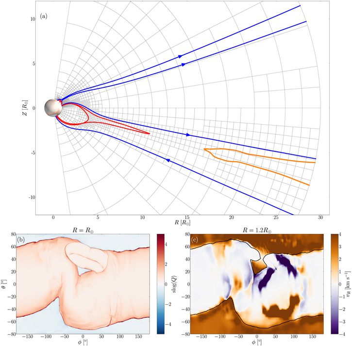
Figure 1. (a) Vertical slice through the simulation domain showing projections of magnetic field lines colored by their connectivity: red—closed, blue—open, orange—disconnected from photosphere. Field direction for the open field lines is indicated by the arrows. Blocks in the simulation grid are denoted by the gray lines. (b) Map of the squashing factor Q at the photosphere. Positive (negative) Q denotes closed (open) magnetic field lines. (c) Radial plasma velocity just above the photosphere showing outflow in the open regions. The black curve indicates the open/closed boundary at the radius indicated. Also visible are some transient upflows and downflows on closed field lines.
Download figure:
Standard image High-resolution imageThe magnetic field line structure in a 2D cut that contains both the helmet streamer and pseudostreamer is shown in Figure 1(a). As is standard, the helmet streamer (shown in red) lies radially beneath the HCS, across which the radial field changes sign (see open field lines that extend down to the solar surface), located in this cut at a latitude around θ = −20°. In the dynamic equilibrium state, the field within the HCS itself is continually opening and closing resulting in the disconnection event shown here between the red and orange field lines. The magnetic field structure that separates the polar coronal hole from the midlatitude coronal hole (located at 20° ≲ θ ≲ 65°, −50° ≲ ϕ ≲ 50°, see Figure 1(b)) is comprised of the separatrix surfaces of three (principal) coronal magnetic null points. The separatrix surfaces of two of these nulls together form a dome that encloses closed magnetic flux (red field lines in Figure 1(a) at around 45° north, and in Figure 3), while a portion of the separatrix of the third (central) null extends as a separatrix curtain out into the heliosphere (Titov et al. 2011). Both spine lines of the eastern and western null points are in the closed field region, meaning that the S-Web structure that partitions the flux of the polar and midlatitude coronal holes is formed entirely by this separatrix surface (Scott et al. 2021). These properties are stable throughout the simulations. Due to the very weak field in the vicinity of the eastern null, different numbers of nulls are found in that region at different times during the simulations due to small-scale fluctuations (that lead to either a null bifurcation or the emergence of a null through the photosphere). For an in-depth discussion of the topology of our relaxed state see Wyper et al. (2021).
We evaluate and visualize the magnetic geometry using the squashing factor Q (Titov et al. 2002), typically displayed on a plane of constant radius (but always calculated between the solar surface and the outer boundary at R = 30R⊙). A positive (negative) sign of Q denotes closed (open) magnetic field lines passing through each point. The distribution of Q in the initial state is shown in Figure 1(b). The magnitude of Q provides a measure of the complexity of the field line mapping in the local vicinity (e.g., Titov et al. 2002). A compact flux tube that passes through one domain boundary corresponds to a low magnitude of Q if it maintains its cross section; it corresponds to a high magnitude of Q if it is highly deformed. It follows that ∣Q∣ tends to infinity at separatrices where the field line mapping is discontinuous (though note that the finite resolution will always lead to a large but finite value of Q in the numerical realization).
The simulation grid extends in radius R from the photosphere at R⊙ to the outer boundary at 30R⊙, in polar angles (latitudes) θ between ±81°, and covers all azimuthal angles (longitudes) ϕ. The simulation grid has been refined where plasma parameters vary strongly and at likely sites for interchange reconnection, such as separatrices. Up to a radius of 1.3R⊙ (which is sufficiently above the top of the pseudostreamer), the entire coronal hole and pseudostreamer are maximally refined. Furthermore, the highest level of refinement follows the open/closed boundary of the northern branch of the helmet streamer (which meets the south of the coronal hole) radially outward—see Figure 1(a).
2.3. Imposed Surface Flows
We impose flows at the lower radial boundary at the photosphere and thereby stimulate field lines to undergo interchange reconnection. The overall flow pattern at the photosphere is made up of circular cells, each of which takes the following divergence-free functional form:


where v0 is a constant,  is the Gaussian function with scaling factor c, centered on (θ, ϕ) = (θc
, ϕc
), and
is the Gaussian function with scaling factor c, centered on (θ, ϕ) = (θc
, ϕc
), and  . Each cell has a time-dependent envelope given by

with a period T and start time t0.
Two sets of 14 such rotational cells are set up in separate locations as shown in Figure 2 whereby the boundaries of (a) the helmet streamer and (b) pseudostreamer are driven in separate simulations. We refer to these simulations hereafter as HS-drive and PS-drive, respectively. We choose similar flow patterns for both simulations, differing mostly by a single translational factor, i.e., the flow pattern at the pseudostreamer has been bodily shifted southwards for the HS-drive simulation. The rotational cells overlap in space, but are staggered to start at three separate times. In both simulations all cells are driven for a single period with T = 20,000 s and have identical values of v0 to give maximum flow speeds of ∼10 km s−1 at the photosphere. This value is chosen as it is much less than characteristic speeds in the corona, and for computational expedience. The identical sign of v0 gives the same rotation direction to all cells and leads to an injection of helicity into the system.
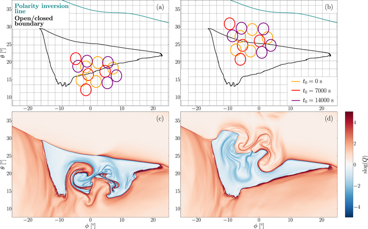
Figure 2. Locations of rotational cells at the photosphere (R = R⊙) relative to the initial (t = 0) open/closed boundary and polarity inversion line for two separate simulations with drive at (a) the helmet streamer and (b) the pseudostreamer. Each cell has a period T = 20,000 s with start times as indicated; note that the circles represent contours of peak velocity and that the cell extends a distance outside it. The gray lines indicate the boundaries of blocks in the computational grid. After the driving has concluded in both cases at t = 10 hr, maps of the squashing factor Q at the photosphere are shown for (c) the HS-drive simulation and (d) the PS-drive simulation.
Download figure:
Standard image High-resolution imageWe note that each of the driving cells is of comparable size to a supergranule. However, this driver is not intended to mimic exactly observed photospheric driving patterns. Detailed analysis (Langfellner et al. 2015) shows that supergranular flows may be decomposed into a pair of diverging/converging and rotational components. The flows in our simulations resemble the former. The latter are excluded as they do not inject substantial complexity into the coronal field, but provide substantial computational challenges for simulations in which the lower boundary is at the photosphere. While the typical flow speed is faster than observed on the photosphere, footpoints of field lines are moved by no more than a supergranular scale under the influence of each vortex, as is the case for real supergranules. However, the characteristics of the overall flow profile are representative of observed flows in the sense that on the Sun the random appearance and disappearance of granular/supergranular convection cells injects twist into the coronal field.
3. Magnetic Field Dynamics and Reconnection
Our purpose here is to explore where and how interchange reconnection occurs, the distribution of newly opened magnetic flux, and implications for the heliospheric field and plasma. We first identify the locations of reconnection in the two simulations by examining the distribution of current in the volume. Although the code solves the ideal MHD equations, numerical dissipation acting on the grid scale permits reconnection where very large gradients of B develop. The particular locations at which reconnection occurs are determined by a combination of the magnetic field topology and the driving.
In response to the boundary driving the coronal field becomes stressed and the geometry of the open/closed boundary (separatrix surfaces) becomes distorted. An isosurface of the current density is shown in Figure 3, for the PS-drive simulation. Filaments of current are seen to extend upwards on the corrugated surface of the separatrix dome from the driven region on the photosphere. In addition, a current accumulation can be seen along the apex of the dome, running from the central null point toward the eastern and western nulls. This corresponds to the location of the separator field line that is formed by the intersection of the null point separatrices. Thus, in line with established theory, reconnection around the nulls and separators is responsible for the opening and closing of flux (Scott et al. 2021, and references therein).
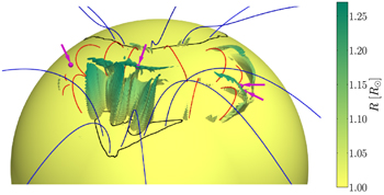
Figure 3. Isosurface of current density at t = 10 hr in the driven pseudostreamer (PS-drive) simulation. The colors indicate height above the photosphere. The instantaneous open/closed boundaries of the coronal holes at the photosphere are indicated by the black lines. Select closed (red) and open (blue) field lines are shown. Four magnetic nulls are denoted by the pink spheres, indicated by similarly colored arrows.
Download figure:
Standard image High-resolution imageFor the HS-drive simulation a similar corrugation occurs, this time of the helmet streamer separatrix surface. This corrugation is found to extend all the way up to the apex of the helmet streamer, indicating that the interchange reconnection occurs in the lower part of the HCS. Although in PFSS models the HCS is a tangential discontinuity of B, here it has a finite width and contains a mixture of closed, open, and disconnected field lines. An example of a closed field line extending up into the HCS that could take part in interchange reconnection with adjacent open field lines is the elongated red field line shown in Figure 1(a).
4. Opening and Closing of Flux by Interchange Reconnection
The prescribed boundary flow advects the footpoints of magnetic field lines at the surface, causing those field lines to exhibit a twist that propagates radially outward. The deformation of the equilibrium field, and in particular, the open/closed boundary can be seen for both sets of flow patterns in the resultant maps of the squashing factor Q; these are shown at t = 36,000 s = 10 hr, after the flows have terminated, in Figures 2(c) and (d), respectively. Under the framework of ideal MHD, we would expect frozen-in field lines to passively maintain their overall topology. In such a case where interchange reconnection is absent, the open/closed boundary would be advected in an identical manner to a set of passive test particles under the influence of a known velocity field (the set of rotational cells).
We can therefore identify field lines that have undergone interchange reconnection as precisely those that deviate from the ideally advected motion at the photosphere (see Aslanyan et al. 2021 for further details). This classification after the surface flows have terminated at t = 10 hr is shown in Figure 4 for both simulations discussed above. Red and blue regions correspond to photospheric plasma elements for which the corresponding coronal field line has the same classification at the start and end of the simulation—closed or open, respectively. The greenish brass-colored plasma elements are threaded by field lines that transition from open to closed during the simulation, while the gray regions on the photosphere correspond to regions of newly opened flux.

Figure 4. Regions of the photosphere (R = R⊙) at t = 36,000 s = 10 hr classified by their magnetic connectivity status as labeled. Note that the unconnected classification is reserved for maps at R > R⊙.
Download figure:
Standard image High-resolution imageIt is clear from the maps of Q (see Figure 2) that the driver at the pseudostreamer and helmet streamer have fundamentally different effects on the magnetic field. The two comparable flow patterns produce a geometrically more complex open/closed boundary when they act on the helmet streamer compared with the pseudostreamer. The reason for this can be understood by considering the different nature of the interchange reconnection process in the two cases. Broadly speaking, the geometry of the open/closed boundary is determined by a balance between the driving—which on average acts to increase the complexity—and the reconnection, which acts to reduce the stored magnetic energy and thus on average reduce the complexity. At the pseudostreamer the reconnection is comparatively efficient, since (i) the reconnection site is low in the corona, and (ii) current sheets that form at nulls and separators are singular in the ideal limit, so that any finite dissipation will lead to reconnection. On the other hand, at the helmet streamer boundary the reconnection site is much higher, and the communication time from the solar surface to the reconnection site low in the HCS is longer. As a result the magnetic stress can be distributed over a much greater length of field lines, and dynamic current sheet thinning will occur over a longer timescale due to the increased communication time. In Figure 2(a), for example, the integrated field line length from photosphere to apex is ∼10R⊙ for the long closed helmet streamer field line and only ∼0.3R⊙ for the closed pseudostreamer field lines.
To quantify the above we obtain the instantaneous form of the open/closed boundary from discretized Q maps with grid size ∼0 02 in both directions, as summarized in Table 1. Surface flows in both simulations lead to an increase in the perimeter of the coronal hole, but it is significantly larger in the HS-drive simulation; the area remains nearly constant in both cases. Taken together, these factors suggest that the magnetic field lines around the pseudostreamer are comparatively more susceptible to interchange reconnection. We anticipate that the higher geometric complexity of the open/closed boundary at the helmet streamer than pseudostreamers should be a general result.
Table 1. Basic Topographic Properties of the Coronal Hole at the Start of the Simulations (t = 0) and After the Surface Flows Have Completed (t = 10 hr) for the Two Simulations
| Boundary | Perimeter [Mm] | Area [Mm2] |
|---|---|---|
| Start | 1243 | 34,502 |
| HS-drive | 2492 | 34,020 |
| PS-drive | 1346 | 33,864 |
Download table as: ASCIITypeset image
Once the connectivity at the photosphere is identified, we can integrate the field lines outward to generate a corresponding map at any arbitrary radius (clearly above a certain radius only open field lines—blue and gray regions—will be present). Such maps at R = 20R⊙ are given in Figures 5(a) and (b) for the HS-drive and PS-drive simulations, respectively. In the context of release of plasma into the solar wind we are particularly interested in field lines that are newly opened (or reconnected open) since the start of the simulation. We overlay the locations of this class of field lines over the normalized current in Figures 5(c) and (d). There is a strong overlap between newly formed current concentrations and regions through which reconnected open field lines pass in both cases. It should be noted that such current concentrations appear to form even in simulations where interchange reconnection does not occur, such as when only the center of the coronal hole is driven. Any statistical links between the two phenomena are to be explored in future simulations and observational studies.

Figure 5. Comparisons of the magnetic connectivity at 20R⊙ for drive at the helmet streamer (left column) and pseudostreamer (right column). The instantaneous connectivity at t = 10 hr is shown in (a) and (b) respectively, colored as in Figure 4 (top row); in particular, the gray regions are threaded by reconnected open field lines, the orange by field lines unconnected to the photosphere. In panels (c) and (d) the regions of reconnected open field lines (gray) are overlaid on the normalized current, showing a broad relation between these phenomena. The total number of times the field lines at each point have changed to or from reconnected open are shown in panels (e) and (f). The solid black curves denote the polarity inversion lines at the end of the simulations, while the dashed curves are separated from it by 2°.
Download figure:
Standard image High-resolution imageFigures 4, 5(a), and 5(b) show the cumulative connectivity change from the start to the end of the driving period at their respective radii. However, it is also instructive to analyze the time history during the simulations, particularly the reconnected open field lines (gray). This is illustrated in Figures 5(e) and (f) in the following manner: starting at the beginning of the simulation until t = 10 hr at each point in space, located at R = 20R⊙, we count the number of times that the field line passing through that point changes its identification to or from reconnected open. The cumulative changes in the connectivity type for each point of latitude and longitude are equivalent to measurements from a corotating spacecraft as field lines sweep past or undergo reconnection. At this radius, the majority of field lines are open in one way or another. Given that none of the field lines begin the simulation as reconnected by definition, a point that ends the simulation threaded by a reconnected open field line must have cumulatively undergone an odd number of such changes.
We observe that interchange-reconnected flux fills a substantial portion of the coronal hole—being found far from the helmet streamer and pseudostreamer—in both simulations. Moreover, we find that this filling occurs unevenly, with many locations observing interchange-reconnected open field lines intermittently as indicated by Figures 5(e) and (f). In other words, connectivity of a given point changes from reconnected open to always open and back again multiple times throughout the evolution. This is particularly apparent in the HS-drive simulation. This is likely to have important consequences for the wind speed on those field lines, discussed further below.
Comparing the results of the PS-drive and HS-drive simulations, we find some large-scale characteristics that are consistent with the predictions made by Aslanyan et al. (2021). First, the newly opened flux is not found at random locations in the heliosphere, but rather in thin fingers or filaments that extend outwards from the corresponding S-Web feature (HS or PS). This was shown by Aslanyan et al. (2021) to be an imprint of the boundary driving, and the length scales of such features should therefore be determined in part by the scale of granular and supergranular driving on the solar surface. Second, the newly opened flux is found further from the original (equilibrium) location of the helmet streamer (for HS-drive) than the pseudostreamer (for PS-drive). This results from a combination of increased expansion factor at the helmet streamer and the greatly increased deformation of the helmet streamer boundary discussed above.
5. Possible in situ Orbital Measurements
5.1. Heliosphere-photosphere Connectivity
A common feature of the two simulations is that newly opened magnetic field lines are found in distinct bundles along the coronal hole boundary (see Figure 4). The extension of these flux bundles out into the heliosphere will form filaments, a series of which may be encountered during a spacecraft fly-through. We simulate such an encounter of a hypothetical spacecraft by choosing a circular orbit at 20R⊙, inclined by −3° so as to pass through the helmet streamer in the HS-drive simulation (Figure 6) and by 8◦ so as to pass through the stalk of the pseudostreamer in the PS-drive simulation (Figure 7). Although it is likely that most spacecraft would orbit the Sun in the ecliptic (i.e., inclined by 0◦), our choice of inclinations can be interpreted as tilting our simulation domain—shifting the midlatitude coronal hole to the north or south. Note that we assume the fly-through to take place instantaneously through our simulation domain at the end of the simulation at t = 10 hr.
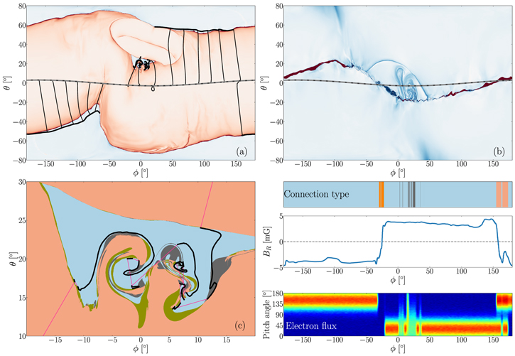
Figure 6. Circular orbit at R = 20R⊙ through the simulation domain at −3° inclination, as indicated by the dashed gray line. (a) Orbit relative to Q at the photosphere, showing magnetic field lines (approximately vertical on the page) connecting the orbit down to a path on the photosphere, as indicated by the solid black lines. (b) Orbit relative to Q at R = 20R⊙. (c) Details of the path on the photosphere in the region of the coronal hole. The narrow pink lines indicate discontinuities in the ground trace. (Lower right) The connection type, magnetic field polarity, and synthetic strahl electron spectrum along this orbit.
Download figure:
Standard image High-resolution image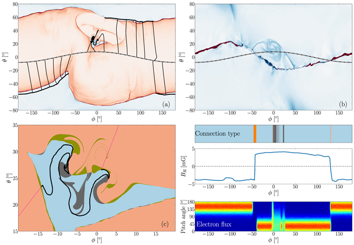
Figure 7. Circular orbit at R = 20R⊙ through the simulation domain at 8◦ inclination, as indicated by the dashed gray line. (a) Orbit relative to Q at the photosphere, showing magnetic field lines (approximately vertical on the page) connecting the orbit down to a path on the photosphere, as indicated by the solid black lines. (b) Orbit relative to Q at R = 20R⊙. (c) Details of the path on the photosphere in the region of the coronal hole. The narrow pink lines indicate discontinuities in the ground trace. (Lower right) The connection type, magnetic field polarity, and synthetic strahl electron spectrum along this orbit.
Download figure:
Standard image High-resolution image
This trajectory is illustrated in panels (a) and (b) of both figures by the dashed gray line. In panel (a) field lines are traced down to the solar surface from selected points on the trajectories. In panel (c) we zoom in to show the detailed ground trace of the spacecraft within the coronal hole.
What is remarkable in both simulations is the complicated geometry of that ground trace, indicating that through time the spacecraft will sample plasma on a field line that is (instantaneously) connected by a footpoint location that meanders through the coronal hole. The convoluted ground trace contrasts sharply with equivalent estimates for connectivity based on a potential field extrapolation for the same photospheric distribution of Br . The true photosphere exhibits magnetic complexity at smaller scales than are resolvable by these simulations, which would exacerbate the erratic ground trace.
For the PS-drive simulation (Figure 7) the ground trace forms a single connected path that transitions multiple times from always open to newly opened field lines. Due to the greater complexity of the open/closed boundary geometry discussed in the previous section, the ground trace of the spacecraft trajectory in the HS-drive simulation is even more complex. In this case the ground trace path appears to exhibits multiple discontinuous jumps (identified by pink lines in Figure 6(c)). In the present simulations these jumps are an artifact of the finite time resolution of our spacecraft trajectory (the mapping can only be discontinuous at a separatrix surface, and none are present at those points). They occur at QSLs in which the mapping has a strong gradient. These layers are found to spread throughout a large portion of the coronal hole open flux as shown, e.g., in Figure 6. In reality there are likely to be open separatrix surfaces embedded within coronal holes, so that truly discontinuous jumps are more common than seen here.
5.2. Implications for Solar Wind Outflow
A spacecraft on one of the trajectories in Figures 6 and 7 could make meaningful deductions about magnetic field connectivity from in situ measurements, even if the full structure and time history of the field remains unknown. In the lower right panel of these two figures we plot both the field line connectivity type and the radial component of the magnetic field along the trajectory. As expected, crossings of the HCS can be identified by a change in the sign of BR , together with the identification of either extended closed field lines or disconnected magnetic flux (i.e., magnetic flux that is not connected to the solar surface). Additionally, for 0° ≲ ϕ ≲ 40°, the connectivity changes multiple times between historically open and newly opened field. In reality, the time-dependent release of closed field plasma onto open field lines would be expected to change the bulk outflow speed on those field lines. Thus the newly opened field lines should exhibit different plasma properties such as flow speed. Due to the simplified isothermal assumption used in our simulations this does not occur, since the plasma in the closed field is not hotter and denser than in the open field. Relaxing this assumption will be undertaken in future work. One way that connectivity is often assessed is to examine the electron strahl. To compare with such observations we have produced synthetic spectra for the electron strahl (shown in the lower right of Figures 6 and 7), taking into account both the connectivity and field polarity. For long-term open field lines (with connectivity labeled blue), we assume strong unidirectional flux at one of two angles depending on the polarity; for closed field lines (labeled red) the flux is bidirectional. For the recently reconnected open field lines (labeled gray), we assume that the flux remains unidirectional, but has been broadened across pitch angles relative to the long-term open field lines.
Looking at the synthetic spectrum in Figure 6, for example, we see a unidirectional signal from open field lines for −180° < ϕ ≲ −50° of the orbit. There follows a brief gap in the strahl due to field lines unconnected to the photosphere as the orbit passes through the HCS, where the field polarity reverses. Just beyond ϕ > 0° are regions of alternating broad and narrow strahl corresponding to open field lines that are intermittently reconnected and not. Further along for ϕ > 150° are bidirectional signals from closed field lines and a second polarity reversal. Detection of intermittent strahl broadening or comparable effects by a real spacecraft, as seen in both the orbits simulated here, would serve to indicate a direct observation of reconnected open field lines.
6. Conclusions
We have presented three-dimensional MHD simulations of the solar corona extended to 30R⊙. The model of interchange reconnection driven by flows mimicking supergranulation includes both a helmet streamer and pseudostreamer. We find key differences in the susceptibility of these two types of magnetic structures to interchange reconnection, with the shorter field lines of a pseudostreamer appearing to reconnect from open to closed more readily than a helmet streamer. The boundary between a coronal hole and a helmet streamer is therefore predicted to be more corrugated and complicated than that of a pseudostreamer.
We confirm that supergranulation at the photosphere causes the localization of interchange-reconnected field lines, and therefore the outflow of closed field plasma, to narrow channels even away from the photosphere. The time history of these field lines is erratic, with many of them reconnecting multiple times or being advected by flowing plasma.
We have used our simulation to show how reconnected field lines may be detected from orbit by signatures in the spectrum of strahl electrons. As a spacecraft passes through the above-mentioned narrow channels of reconnected flux, we posit that it would detect a periodic variation in the fast electron pitch angles. We show that the track of orbit-connected magnetic field lines at the photosphere may be significantly more complicated than those predicted by pure PFSS models.
Our results have critical implications for observations and modeling of the Sun-heliosphere connection. With respect to the magnetic field connectivity, it is evident from Figures 6 and 7 that once the effects of photospheric dynamics are included, then even with in situ measurements close to the Sun, such as those from PSP and SO, determining the exact photospheric locations of the footpoints of heliospheric field lines is unlikely to be possible. The satellite footpoint-trajectories of Figures 6 and 7 have too much fine structure to resolve and this fine structure will inevitably change rapidly in time as a result of interchange reconnection. We conclude that near open/closed boundaries, the magnetic connectivity can be determined only in an approximate sense, over the scale of a supergranule or so. This conclusion will be even more valid for the plasma connectivity. A long-standing goal of missions like PSP and SO is to connect the properties of some parcel of plasma measured in situ in the heliosphere with the plasma properties determined via remote sensing observations of its coronal origins. Our results imply that this origin can be determined only down to the scale of a supergranule, which may introduce considerable uncertainty in the initial coronal properties of the heliospheric plasma.
Another important implication of our results pertains to models of the so-called switchbacks (Bale et al. 2019). Several authors have proposed that their origin is due to interchange reconnection (e.g., Drake et al. 2021; Liang et al. 2021). We do find copious interchange reconnection at the open/closed boundary and this reconnection is structured by the supergranular flows, in agreement with the recent observations (Fargette et al. 2021). Our present simulations, however, have too low spatial resolution to capture accurately important structures, such as magnetic plasmoids, formed during the reconnection. Furthermore, the simulations do not include key plasma thermodynamics such as thermal conduction and radiation, so they cannot be expected to produce switchbacks. We suggest, however, that future simulations very similar to those above, but with higher resolution and more realistic plasma energetics, will be able to make a definitive determination of whether interchange reconnection is, in fact, the origin of the highly intriguing phenomenon of switchbacks.
This work was performed using resources provided by the Cambridge Service for Data Driven Discovery (CSD3) operated by the University of Cambridge Research Computing Service, provided by Dell EMC and Intel using Tier-2 funding from the Engineering and Physical Sciences Research Council (capital grant EP/P020259/1), and DiRAC funding from the Science and Technology Facilities Council. V.A. is supported by the Science and Technology Facilities Council, grant No. ST/S000267. R.B.S. is supported by the Office of Naval Research 6.1 basic research program. A.K.H. and R.B.S. were in part supported by the NASA Parker Solar Probe WISPR program. S.K.A. was supported by the NASA LWS Program.