Pressure–Strain Interaction as the Energy Dissipation Estimate in Collisionless Plasma

The picture of turbulence cascade as developed by Taylor, von Kármán, Kolomogorov, and others (de Kármán & Howarth 1938; Taylor 1938; Kolmogorov 1941a, 1941b) describes energy transfer across scales from an energy-containing range, through an inertial range and into a dissipation range where fluctuations are converted into internal energy. This basic picture is readily adapted to magnetohydrodynamics (MHD; Biskamp 2003), a magnetofluid model (Moffatt 1978) often applied as an approximation to low-density high-temperature cosmic plasmas (Parker 1979) such as the solar wind (Breech et al. 2008). Recently there has been increasing interest in advancing descriptions of turbulence in more complex plasma models (Bowers & Li 2007; Parashar et al. 2009; Howes et al. 2011). In particular there is impetus to understand dissipation for kinetic plasmas in which the classical collisional approach becomes inapplicable, and therefore also inapplicable are standard closures that capture dissipation as empirical descriptions in terms of fluid scale variables. Fortunately, instead of studying specific dissipative mechanisms at kinetic scales, such as wave–particle interactions (Hollweg 1986; Hollweg & Isenberg 2002; Gary & Saito 2003; Markovskii et al. 2006; Gary et al. 2008; Howes et al. 2008; Chandran et al. 2010; He et al. 2015), field–particle correlations (Klein & Howes 2016; Chen et al. 2019; Klein et al. 2020), or heating by coherent structures and reconnection (Dmitruk et al. 2004; Retinò et al. 2007; Sundkvist et al. 2007; Parashar et al. 2011; Perri et al. 2012; TenBarge & Howes 2013; He et al. 2018), an alternative strategy based on the energy transfer process is available. One can proceed by tracing available pathways that lead to deposition of internal (or thermal) energy. "Dissipation" here simply refers to a degradation of fluid scale and electromagnetic fluctuations into internal energy (Matthaeus et al. 2020). This increase in internal energy is eventually "thermalized" by collisions and entropy production (Liang et al. 2019; Pezzi et al. 2019a), but this irreversibility is not our focus here.

Different dissipation proxies based on the energy transfer process have been adapted to estimate the dissipation rate. A von Kármán–Howarth picture (de Kármán & Howarth 1938) of turbulent decay was extended for MHD (Hossain et al. 1995; Wan et al. 2012b), in which the global decay rate of energy is controlled by the von Kármán decay law at energy-containing scales (Wan et al. 2012b; Wu et al. 2013; Zank et al. 2017; Bandyopadhyay et al. 2018c, 2018b, 2019). The energy dissipation rate is estimated by the energy decay rate. The energy loss at energy-containing scales is then transferred across scales in the MHD inertial range. To obtain the inertial range energy transfer rate, the Yaglom relation (Politano & Pouquet 1998; Sorriso-Valvo et al. 2007; Stawarz et al. 2009; Coburn et al. 2015; Bandyopadhyay et al. 2018a) and its extensions (Podesta 2008; Wan et al. 2009; Osman et al. 2011; Banerjee & Galtier 2013; Verdini et al. 2015; Hadid et al. 2017; Hellinger et al. 2018; Andrés et al. 2019; Ferrand et al. 2019, 2022) have been adapted, in which the energy dissipation rate is estimated by the energy transfer rate. The transferred energy ultimately goes into the internal energy reservoir, which is often evaluated by the rate of work done by the electric field on particles for species α, j _α · E (Zenitani et al. 2011; Wan et al. 2012a, 2015; Chasapis et al. 2018a; Ergun et al. 2018; Phan et al. 2018; Lu et al. 2019; Vörös et al. 2019; Pongkitiwanichakul et al. 2021) and more recently by the pressure–strain interaction for species α, $-\left({{\boldsymbol{P}}}_{\alpha }\cdot {\rm{\nabla }}\right)\cdot {{\boldsymbol{u}}}_{\alpha }$ (Yang et al. 2017a, 2017b; Chasapis et al. 2018b; Sitnov et al. 2018; Yang 2019; Zhong et al. 2019; Bandyopadhyay et al. 2020a; Jiang et al. 2021; Bacchini et al. 2022).

One observable feature is that the aforementioned dissipation rate estimates dominate at different scales. Two standard ways to disentangle the multiscale properties in configuration space are scale-filtering representations and lag dependent structure functions. Scale filter (Germano 1992) is based on real space coarse-graining at a specified length scale, which is widely used in Large Eddy Simulation computational methods (Meneveau & Katz 2000; Pope 2004), in analytical theory (Eyink 2003; Aluie 2013), and recently in promising applications to turbulence in plasma models (Yang et al. 2017a; Camporeale et al. 2018; Eyink 2018; Yang et al. 2019; Cerri & Camporeale 2020; Teaca et al. 2021). Structure functions such as the von Kármán–Howarth relation (de Kármán & Howarth 1938; Monin & Yaglom 1975), defined in terms of increments, have a long history in turbulence theory (Frisch 1995). Here we are concerned with energy balance across scales, measured using the von Kármán–Howarth equation (Verdini et al. 2015; Hellinger et al. 2018; Ferrand et al. 2019; Adhikari et al. 2021) and filtered Vlasov–Maxwell equations (Yang et al. 2017a; Matthaeus et al. 2020). In both scale-filtering and structure function representations, crucial elements are energy loss at large scales, energy flux in an intermediate range, and dissipation at small scales. So we compare corresponding scale filtered and structure function decompositions and clarify the relationship between energy dissipation estimates at different scales.

A number of studies have been devoted to investigate the multiplicity of dissipation rate estimates (Yang et al. 2019; Bandyopadhyay et al. 2020b; Matthaeus et al. 2020; Pezzi et al. 2021; Bandyopadhyay et al. 2021; Zhou et al. 2021). In this paper, we specifically address the role of the pressure–strain interaction for species α, $-\left({{\boldsymbol{P}}}_{\alpha }\cdot {\rm{\nabla }}\right)\cdot {{\boldsymbol{u}}}_{\alpha }$, in two aspects. On the one hand, different pathways contributing to the global evolution of energies are traced, as used in Du et al. (2018) Pezzi et al. (2019b) Song et al. (2020), and Bacchini et al. (2022), which illustrates the difference between $-\left({{\boldsymbol{P}}}_{\alpha }\cdot {\rm{\nabla }}\right)\cdot {{\boldsymbol{u}}}_{\alpha }$ and j _α · E . On the other hand, the scale decomposition of these pathways is realized using the von Kármán–Howarth equation and filtered Vlasov–Maxwell equations, which illustrates the relationship among the von Kármán decay law, the Yaglom relation, and $-\left({{\boldsymbol{P}}}_{\alpha }\cdot {\rm{\nabla }}\right)\cdot {{\boldsymbol{u}}}_{\alpha }$. We make a detailed comparison of these elements using kinetic plasma simulations. Major findings are: first, that the potential deficiency of the Yaglom relation for estimation of the dissipation rate, especially for the turbulence without well-defined inertial range, is exemplified; second, that energy balance across scales is established, even when the Yaglom relation and its subsidiary assumptions are not valid; and third, that the quantitatively correct description of dissipation in kinetic plasma is that computed from the pressure–strain interaction.

2.1. Energy Balance Equations

There are multiple forms of energy available for participation in energy transfer in collisionless plasma. These include: electromagnetic energy ${E}^{m}=\left({{\boldsymbol{B}}}^{2}+{{\boldsymbol{E}}}^{2}\right)/(8\pi )$, where B and E are magnetic and electric fields; fluid flow kinetic energy of species α ${E}_{\alpha }^{f}={\rho }_{\alpha }{{\boldsymbol{u}}}_{\alpha }^{2}/2$, where ρ_α is the mass density and u _α is the fluid velocity; and corresponding internal energy ${E}_{\alpha }^{\mathrm{th}}=\tfrac{1}{2}{m}_{\alpha }\int {\left({\boldsymbol{v}}-{{\boldsymbol{u}}}_{\alpha }\right)}^{2}{f}_{\alpha }\left({\boldsymbol{x}},{\boldsymbol{v}},t\right)d{\boldsymbol{v}}$, with mass m_α and velocity distribution function f_α . The first three moments of the Vlasov equation, in conjunction with the Maxwell equations, yield the time evolution of the energies:

$$\begin{eqnarray}&&{\partial }_{t}{E}_{\alpha }^{f}+{\rm{\nabla }}\cdot \left({E}_{\alpha }^{f}{{\boldsymbol{u}}}_{\alpha }+{{\boldsymbol{P}}}_{\alpha }\cdot {{\boldsymbol{u}}}_{\alpha }\right)=\left({{\boldsymbol{P}}}_{\alpha }\cdot {\rm{\nabla }}\right)\cdot {{\boldsymbol{u}}}_{\alpha }+{{\boldsymbol{j}}}_{\alpha }\cdot {\boldsymbol{E}},\end{eqnarray} \tag{ 1 }$$

$$\begin{eqnarray}&&{\partial }_{t}{E}_{\alpha }^{\mathrm{th}}+{\rm{\nabla }}\cdot \left({E}_{\alpha }^{\mathrm{th}}{{\boldsymbol{u}}}_{\alpha }+{{\boldsymbol{h}}}_{\alpha }\right)=-\left({{\boldsymbol{P}}}_{\alpha }\cdot {\rm{\nabla }}\right)\cdot {{\boldsymbol{u}}}_{\alpha },\end{eqnarray} \tag{ 2 }$$

$$\begin{eqnarray}&&{\partial }_{t}{E}^{m}+\displaystyle \frac{c}{4\pi }{\rm{\nabla }}\cdot \left({\boldsymbol{E}}\times {\boldsymbol{B}}\right)=-{\boldsymbol{j}}\cdot {\boldsymbol{E}},\end{eqnarray} \tag{ 3 }$$

where the subscript α = e, i represents the species, P _α is the pressure tensor, h _α is the heat flux vector, j = ∑_α j _α is the total electric current density, j _α = n_α q_α u _α is the electric current density of species α, and n_α and q_α are the number density and the charge of species α, respectively. Note that the spatial transport terms (i.e., the second terms on the left-hand side) are globally conservative and cancel out under certain boundary conditions, e.g., periodic.

From these equations, one can see the roles of several energy transfer pathways. For example, the electric work, j _α · E , exchanges electromagnetic energy with fluid flow energy for species α, while the pressure–strain interaction, $-\left({{\boldsymbol{P}}}_{\alpha }\cdot {\rm{\nabla }}\right)\cdot {{\boldsymbol{u}}}_{\alpha }$, represents the conversion between fluid flow and internal energy for species α. The pressure–strain interaction can be further decomposed as

$$\begin{eqnarray}&&\langle -\left({{\boldsymbol{P}}}_{\alpha }\cdot {\rm{\nabla }}\right)\cdot {{\boldsymbol{u}}}_{\alpha }\rangle =\langle -{p}_{\alpha }{\rm{\nabla }}\cdot {{\boldsymbol{u}}}_{\alpha }-{{\boldsymbol{\Pi }}}_{\alpha }:{{\boldsymbol{D}}}_{\alpha }\rangle =p{\theta }_{\alpha }+{{PiD}}_{\alpha },\end{eqnarray} \tag{ 4 }$$

where 〈 ⋯ 〉 denotes spatial average, p_α = P_α,ii /3, Π_α,ij = P_α,ij − p_α δ_ij , and ${D}_{\alpha ,{ij}}=\left({\partial }_{i}{u}_{\alpha ,j}+{\partial }_{j}{u}_{\alpha ,i}\right)/2-\,\left({\rm{\nabla }}\cdot {{\boldsymbol{u}}}_{\alpha }\right){\delta }_{{ij}}/3$. p θ_α and PiD_α denote compressible and incompressible parts, respectively.

2.2. Scale-filtering Representation

To disentangle the scale-by-scale dynamics, it is useful to define a filter (Germano 1992) at scale ℓ, operating on the velocity and electromagnetic fields. With a properly defined filtering kernel ${G}_{{\ell }}\left({\boldsymbol{r}}\right)={{\ell }}^{-d}G\left({\boldsymbol{r}}/{\ell }\right)$, where d is the spatial dimension and $G\left({\boldsymbol{r}}\right)$ is a nonnegative and normalized boxcar window function so that ∫d^d rG( r ) = 1, the field f( x , t) is filtered at scale ℓ as

$$\begin{eqnarray*}&&\begin{array}{l}{\bar{f}}_{{\ell }}({\boldsymbol{x}},t)=\int {d}^{d}{{rG}}_{{\ell }}({\boldsymbol{r}})f({\boldsymbol{x}}+{\boldsymbol{r}},t).\end{array}\end{eqnarray*}$$

The low-pass filtered ${\bar{f}}_{{\ell }}({\boldsymbol{x}},t)$ only contains information at length scales ≥ ℓ. The Favre-filtered (density-weighted-filtered) field (Favre 1969) is defined as

$$\begin{eqnarray*}&&\begin{array}{l}{\tilde{f}}_{{\ell }}={\overline{\rho f}}_{{\ell }}/{\bar{\rho }}_{{\ell }}.\end{array}\end{eqnarray*}$$

We drop the subscript ℓ for notation simplicity. An overbar $\bar{f}$ denotes a filtered quantity, and a tilde $\tilde{f}$ denotes a density-weighted (Favre) filtered quantity.

Proceeding with the Vlasov–Maxwell equations, the resolved kinetic and electromagnetic energy equations at scale ℓ (Yang et al. 2017a; Eyink 2018; Matthaeus et al. 2020) are

$$\begin{eqnarray}&&{\partial }_{t}{\widetilde{E}}_{\alpha }^{f}+{\rm{\nabla }}\cdot {{\boldsymbol{J}}}_{\alpha }^{u}=-{{\rm{\Pi }}}_{\alpha }^{{uu}}-{{\rm{\Phi }}}_{\alpha }^{{uT}}-{{\rm{\Lambda }}}_{\alpha }^{{ub}},\end{eqnarray} \tag{ 5 }$$

$$\begin{eqnarray}&&{\partial }_{t}{\overline{E}}^{m}+{\rm{\nabla }}\cdot {{\boldsymbol{J}}}^{b}=-\sum _{\alpha }{{\rm{\Pi }}}_{\alpha }^{{bb}}+\sum _{\alpha }{{\rm{\Lambda }}}_{\alpha }^{{ub}},\end{eqnarray} \tag{ 6 }$$

where ${\widetilde{E}}_{\alpha }^{f}=\tfrac{1}{2}{\bar{\rho }}_{\alpha }{\tilde{{\boldsymbol{u}}}}_{\alpha }^{2}$ is the filtered fluid flow energy; ${\overline{E}}^{m}=({\bar{{\boldsymbol{B}}}}^{2}+{\bar{{\boldsymbol{E}}}}^{2})/(8\pi )$ is the filtered electromagnetic energy; ${{\boldsymbol{J}}}_{\alpha }^{u}\,={\widetilde{E}}_{\alpha }^{f}{\tilde{{\boldsymbol{u}}}}_{\alpha }+{\bar{\rho }}_{\alpha }{\tilde{{\boldsymbol{\tau }}}}_{\alpha }^{u}\cdot {\tilde{{\boldsymbol{u}}}}_{\alpha }+{\overline{{\boldsymbol{P}}}}_{\alpha }\cdot {\tilde{{\boldsymbol{u}}}}_{\alpha }$ and ${{\boldsymbol{J}}}^{b}=\left(c\overline{{\boldsymbol{E}}}\times \overline{{\boldsymbol{B}}}\right)/(4\pi )$ are the spatial transport; ${{\rm{\Pi }}}_{\alpha }^{{uu}}=-\left({\bar{\rho }}_{\alpha }{\tilde{{\boldsymbol{\tau }}}}_{\alpha }^{u}\cdot {\rm{\nabla }}\right)$ $\cdot {\tilde{{\boldsymbol{u}}}}_{\alpha }-{q}_{\alpha }/c{\bar{n}}_{\alpha }{\tilde{{\boldsymbol{\tau }}}}_{\alpha }^{b}\cdot {\tilde{{\boldsymbol{u}}}}_{\alpha }$ is the sub-grid-scale (SGS) flux of fluid flow energy across scales due to nonlinearities, where ${\tilde{{\boldsymbol{\tau }}}}_{\alpha }^{u}=\widetilde{{{\boldsymbol{u}}}_{\alpha }{{\boldsymbol{u}}}_{\alpha }}-{\tilde{{\boldsymbol{u}}}}_{\alpha }{\tilde{{\boldsymbol{u}}}}_{\alpha }$, ${\tilde{{\boldsymbol{\tau }}}}_{\alpha }^{b}=\widetilde{{{\boldsymbol{u}}}_{\alpha }\times {\boldsymbol{B}}}-{\tilde{{\boldsymbol{u}}}}_{\alpha }\times \tilde{{\boldsymbol{B}}};$ ${{\rm{\Pi }}}_{\alpha }^{{bb}}=-{q}_{\alpha }{\bar{n}}_{\alpha }{\tilde{{\boldsymbol{\tau }}}}_{\alpha }^{e}\cdot {\tilde{{\boldsymbol{u}}}}_{\alpha }$ is the SGS flux of electromagnetic energy across scales due to nonlinearities, where ${\tilde{{\boldsymbol{\tau }}}}_{\alpha }^{e}=\tilde{{\boldsymbol{E}}}-\bar{{\boldsymbol{E}}};$ ${{\rm{\Phi }}}_{\alpha }^{{uT}}=-\left({\overline{{\boldsymbol{P}}}}_{\alpha }\cdot {\rm{\nabla }}\right)\cdot {\tilde{{\boldsymbol{u}}}}_{\alpha }$ is the rate of flow energy converted into internal energy through filtered $-\left({{\boldsymbol{P}}}_{\alpha }\cdot {\rm{\nabla }}\right)\cdot {{\boldsymbol{u}}}_{\alpha };$ ${{\rm{\Lambda }}}_{\alpha }^{{ub}}=-{q}_{\alpha }{\bar{n}}_{\alpha }\widetilde{{\boldsymbol{E}}}\cdot {\tilde{{\boldsymbol{u}}}}_{\alpha }$ is the rate of conversion of fluid flow energy into electromagnetic energy through filtered − j _α · E .

We can avoid the complication of the interchange between fluid flow and electromagnetic energy and the spatial transport by summing Equations (5) and (6) over species and averaging over space, which yields

$$\begin{eqnarray}&&\mathop{\underbrace{{\partial }_{t}\left\langle \sum _{\alpha }{\widetilde{E}}_{\alpha }^{f}+{\overline{E}}^{m}\right\rangle }}\limits_{{T}_{f}-\epsilon }=-\mathop{\underbrace{\left\langle \sum _{\alpha }\left({{\rm{\Pi }}}_{\alpha }^{{uu}}+{{\rm{\Pi }}}_{\alpha }^{{bb}}\right)\right\rangle }}\limits_{{F}_{f}}-\mathop{\underbrace{\left\langle \sum _{\alpha }{{\rm{\Phi }}}_{\alpha }^{{uT}}\right\rangle }}\limits_{{D}_{f}}.\end{eqnarray} \tag{ 7 }$$

The spatial transport terms are globally conservative under suitable boundary conditions, e.g., periodic. is the total dissipation rate. In the absence of an exact expression of dissipation in collisionless plasma simulations, the dissipation rate is computed by $\epsilon =-d\left\langle {\sum }_{\alpha }{E}_{\alpha }^{f}+{E}^{m}\right\rangle /{dt}$. The first term is the time-rate-of-change of energy at scales ≥ ℓ, which is 0 at large enough ℓ and − at ℓ → 0. In analogy with the structure function representation in Section 2.3, the first term is written as ${T}_{f}=\epsilon +{\partial }_{t}\left\langle {\sum }_{\alpha }{\widetilde{E}}_{\alpha }^{f}+{\overline{E}}^{m}\right\rangle$, which is the time-rate-of-change of energy at scales < ℓ and equals at large enough ℓ (e.g., larger than energy-containing scales) and 0 at ℓ → 0. The remaining terms are the nonlinear cross-scale energy flux F_f and the deposition of internal energy received from the cascade D_f . Similar to Equation (4), the filtered pressure–strain interaction is decomposed as

$$\begin{eqnarray}&&\begin{array}{l}\langle {{\rm{\Phi }}}_{\alpha }^{{uT}}\rangle =\langle -\left({\overline{{\boldsymbol{P}}}}_{\alpha }\cdot {\rm{\nabla }}\right)\cdot {\tilde{{\boldsymbol{u}}}}_{\alpha }\rangle =\langle -{\bar{p}}_{\alpha }{\rm{\nabla }}\cdot {\tilde{{\boldsymbol{u}}}}_{\alpha }\rangle -\langle {\overline{{\boldsymbol{\Pi }}}}_{\alpha }:{\widetilde{{\boldsymbol{D}}}}_{\alpha }\rangle \\ \quad =\ {\overline{p\theta }}_{\alpha }+{\overline{{PiD}}}_{\alpha }.\end{array}\end{eqnarray} \tag{ 8 }$$

2.3. Structure Function Representation

The energy distribution among scales can also be defined by considering two-point correlations or the related second-order structure functions. We proceed with the incompressible Hall MHD model due to its relative analytical simplicity. The associated von Kármán–Howarth equation (de Kármán & Howarth 1938; Monin & Yaglom 1975; Verdini et al. 2015; Hellinger et al. 2018; Ferrand et al. 2019; Adhikari et al. 2021) in structure function form is

$$\begin{eqnarray}&&\begin{array}{l}\mathop{\underbrace{{\partial }_{t}S({\ell })/4}}\limits_{-{T}_{s}}+\mathop{\underbrace{{{\rm{\nabla }}}_{{\ell }}\cdot \left[{\boldsymbol{Y}}({\ell })/4+{\boldsymbol{H}}({\ell })/8\right]}}\limits_{-{F}_{s}}\\ \quad =\ -\epsilon +\mathop{\underbrace{{D}_{\mu }({\ell })+{D}_{\eta }({\ell })}}\limits_{{D}_{s}},\end{array}\end{eqnarray} \tag{ 9 }$$

where ℓ is the spatial lag, ∇_ℓ is the gradient with respect to the lag ℓ, $S({\ell })=\langle \rho {\left(\delta {\boldsymbol{u}}\right)}^{2}\rangle +\langle {\left(\delta {\boldsymbol{B}}\right)}^{2}\rangle$ is a second-order structure function, u is the bulk fluid velocity, and δ u = u ( x + ℓ) − u ( x ) defines the increment. ${\boldsymbol{Y}}({\ell })=\langle {\left(\delta {\boldsymbol{u}}\right)}^{2}\delta {\boldsymbol{u}}+{\left(\delta {\boldsymbol{B}}\right)}^{2}\delta {\boldsymbol{u}}-2\left(\delta {\boldsymbol{B}}\cdot \delta {\boldsymbol{u}}\right)\delta {\boldsymbol{B}}\rangle$ is a third-order structure function, ${\boldsymbol{H}}({\ell })=\langle 2\left(\delta {\boldsymbol{B}}\cdot \delta {\boldsymbol{j}}\right)\delta {\boldsymbol{B}}-{\left(\delta {\boldsymbol{B}}\right)}^{2}\delta {\boldsymbol{j}}\rangle$ is the Hall term, and ${D}_{\mu }({\ell })=\mu {{\rm{\nabla }}}_{{\ell }}^{2}\langle {\left(\delta {\boldsymbol{u}}\right)}^{2}\rangle /2$ and ${D}_{\eta }({\ell })=\eta {{\rm{\nabla }}}_{{\ell }}^{2}\langle {\left(\delta {\boldsymbol{B}}\right)}^{2}\rangle /2$ are the viscous and resistive terms, respectively.

Several points concerning Equation (9) warrant clarification. First, the terms in Equation (9) are functions of lag vector (ℓ_x , ℓ_y , ℓ_z ). Upon averaging over directions, the terms in Equation (9) only depend on lag length ℓ, and T_s , F_s , and D_s denote omnidirectional forms of the three terms in Equation (9). Second, Equation (9) refers to a fluid model, so u = (m_i n_i u _i + m_e n_e u _e )/(m_i n_i + m_e n_e ) and ρ = m_i n_i + m_e n_e are dominated by contributions from ions. Third, for the incompressible model used here, we neglect the spatial and time variability of density and set it to be a constant that equals the spatially and temporally averaged density. The kinetic plasma simulations used here are weakly compressed, which are shown in detail in Sections 4 and 5. The incompressible model therefore remains a credible approximation for our simulations. For strongly compressed plasmas, e.g., the turbulent magnetosheath, more elaborate compressive models (Banerjee & Galtier 2013; Hadid et al. 2017; Andrés et al. 2019; Ferrand et al. 2022) are required. Next, the interpretation of S/4 is that it is related to the energy at scales < ℓ. To see this, let the lag ℓ → 0, so that S/4 tends to zero, while it equals the fluid flow and magnetic energy at large ℓ. The second term F_s measures the energy flux through the surface of a lag sphere of radius ℓ. Finally, the viscous and resistive term D_s has the property that for incompressible MHD, it converges to the dissipation rate = μ〈∇ u : ∇ u 〉 + η〈∇ b : ∇ b 〉 in the limit ℓ → 0. Since this study proceeds with kinetic plasma simulations, we cannot compute and D_s directly, which instead are derived by $\epsilon =-d\left\langle {\sum }_{\alpha }{E}_{\alpha }^{f}+{E}^{m}\right\rangle /{dt}$ and D_s = − T_s − F_s .

2.4. Association with Dissipation Rate Estimates

To appreciate the physical content of the comparisons below, it is necessary to understand both the differences and the similarities of the energy balance of Equations (1)–(3), the scale-filtering formulation in Equation (7) and the structure function formulation of Equation (9), and their associations with the dissipation rate. The energy balance equations show direct causality between the global evolutions of energies and j _α · E and $-\left({{\boldsymbol{P}}}_{\alpha }\cdot {\rm{\nabla }}\right)\cdot {{\boldsymbol{u}}}_{\alpha }$, while the scale-filtering and structure function formulations show details of energy distributions and dissipation proxies across scales.

The scale filter as implemented in Equation (7) contains the scale-decomposed energy budget of the full Vlasov–Maxwell model. This includes compressive and wave–particle effects and contributions from both protons and electrons. The structure function model as implemented in Equation (9) is a purely fluid construct (incompressible Hall MHD). As such it lacks compressible effects, wave–particle interactions, and other non-Hall kinetic effects. Therefore, we anticipate that the correspondence between Equations (7) and (9) may remain credible at MHD scales, identified tentatively as scales larger than ion inertial length.

Even still, the scale-decomposed formulations share common elements in the physics they represent. Both are expressions of conservation of energy across scales and are composed of (i) the rate-of-change of energy at scales < ℓ, T_f , and T_s ; (ii) energy transfer across scale ℓ, F_f , and F_s , leading to the possibility of an inertial range; and (iii) measures of energy dissipation, D_f , and D_s . These elements are in direct association with energy dissipation proxies based on the energy transfer process. For example, the time derivative terms T_f and T_s at energy-containing ℓ represent the energy decay rate, which can be taken as a dissipation estimate. According to the von Kármán decay law (Wan et al. 2012b; Wu et al. 2013; Zank et al. 2017; Bandyopadhyay et al. 2018b, 2019),

$$\begin{eqnarray}&&{\epsilon }_{{vK},\pm }=-\displaystyle \frac{d{({Z}^{\pm })}^{2}/2}{{dt}}=\displaystyle \frac{{\alpha }_{\pm }}{2}\displaystyle \frac{{({Z}^{\pm })}^{2}{Z}^{\mp }}{{L}_{\pm }},\end{eqnarray} \tag{ 10 }$$

where α_± are positive constants, Z^± are the rms fluctuation values of the Elsässer variables, and L_± are similarity length scales (correlation lengths are usually used); the energy decay rate is given by _vK = (_vK,+ + _vK,−)/2. The terms F_f and F_s are related to the inertial range energy transfer rate, giving rise to the widely used Yaglom relation (Politano & Pouquet 1998; Sorriso-Valvo et al. 2007; Stawarz et al. 2009; Coburn et al. 2015; Verdini et al. 2015; Bandyopadhyay et al. 2018a)

$$\begin{eqnarray}&&{\epsilon }_{{Ym}}=-{{\rm{\nabla }}}_{{\ell }}\cdot \left(\displaystyle \frac{{\boldsymbol{Y}}}{4}+\displaystyle \frac{{\boldsymbol{H}}}{8}\right),\end{eqnarray} \tag{ 11 }$$

which can be taken as a dissipation estimate. Although the exact expression of D_s is not known in our kinetic plasma simulations, the term D_f shown in Equation (7) is the spatial average of the filtered pressure–strain interaction, which can estimate the fluid flow energy conversion into internal energy.

In summary, the intent of energy balance equations in Section 2.1 is to illuminate global behaviors, while the scale-filtering and structure function representations in Sections 2.2 and 2.3 aim at scale dependence. Detailed treatments based on the three aforementioned formulations are useful to describe the extent to which these dissipation proxies are correlated and their domain of validity.

Vlasov–Maxwell solutions are obtained with particle in cell (PIC) codes; for run parameters, see Table 1. Here we make use of 2.5D and 3D kinetic simulations with no external drive. So both are decaying initial value problems.

Table 1. 2.5D and 3D PIC Simulation Parameters: Domain Size L; Grid Points in Each Direction N; Ion-to-electron Mass Ratio m_i /m_e ; Guide Magnetic Field in Z-direction B₀; Initial Magnetic Fluctuation Amplitude δ b; Plasma β; Average Number of Particles of Each Species per Grid ppg

Dimension	L(di )	N	mi /me	${B}_{0}\hat{z}$	δ b/B0	β	ppg
2.5D	150	4096	25	1.0	0.5	0.6	3200
3D	42	2048	50	0.5	1.0	0.5	150

Download table as:  ASCIITypeset image

The 2.5D case was performed using the code P3D (Zeiler et al. 2002) in a 2.5D geometry with turbulent fluctuations in (x, y) plane but no variation in the z-direction. All physical quantities have all three components of the vectors. The simulation was performed in a periodic domain, whose size is L ≃ 150d_i , where d_i is the ion inertial length, with 4096² grid points and 3200 particles of each species per cell (∼1.07 × 10¹¹ total particles). The ion-to-electron mass ratio is m_i /m_e = 25, and the ratio ω_pe /ω_ce = 3, where ω_pe is the electron plasma frequency and ω_ce is the electron cyclotron frequency. The run was started with uniform density n₀ = 1.0 and Maxwellian-distributed ions and electrons with temperature T₀ = 0.3. The uniform magnetic field is B₀ = 1.0 directed out of the plane, and plasma β = 0.6. The velocity and magnetic perturbations are transverse to B₀, typical of "Alfvénic" modes. They were seeded at time t = 0 by populating Fourier modes for a range of wavenumbers 2 ≤∣ k ∣ ≤ 4 with random phased fluctuations and a specific spectrum. The run was evolved for more than $300{\omega }_{{ci}}^{-1}$. This simulation was also used in Parashar et al. (2018), Yang et al. (2019), Matthaeus et al. (2020), and Bandyopadhyay et al. (2021).

The 3D case was obtained using the VPIC code (Bowers et al. 2008). The simulation was conducted in a fully periodic 3D domain of size L ≃ 42d_i with resolution of 2048³ cells and 150 particles per cell per species (∼2.6 × 10¹² total particles). The ion-to-electron mass ratio is m_i /m_e = 50, and the ratio ω_pe /ω_ce = 2. The initial conditions correspond to uniform plasma with density n₀, Maxwellian-distributed ions and electrons of equal temperature T₀, uniform magnetic field B₀ in the z-direction, and plasma β = 0.5. Turbulent fluctuations were seeded at time t = 0 by imposing a large-scale isotropic spectrum of velocity and magnetic fluctuations having polarizations transverse to the guide magnetic field B₀. The run was evolved for about $170{\omega }_{{ci}}^{-1}$. Further details of this simulation can be found in V. Roytershteyn et al. (2014, in preparation).

We study the time evolution of global volume averages of energy to find the electromagnetic work 〈 j _α · E 〉 versus the pressure–strain interaction $\langle -\left({{\boldsymbol{P}}}_{\alpha }\cdot {\rm{\nabla }}\right)\cdot {{\boldsymbol{u}}}_{\alpha }\rangle$, the incompressive PiD_α versus compressive p θ_α conversion of energy, and ion (α = i) versus electron (α = e) heating. Accurate integrals of energy transfer pathways over time require small time steps, and this time-integrated procedure is rather expensive for the 3D PIC simulation. Therefore, the analysis in this section is only conducted using the 2.5D PIC simulation.

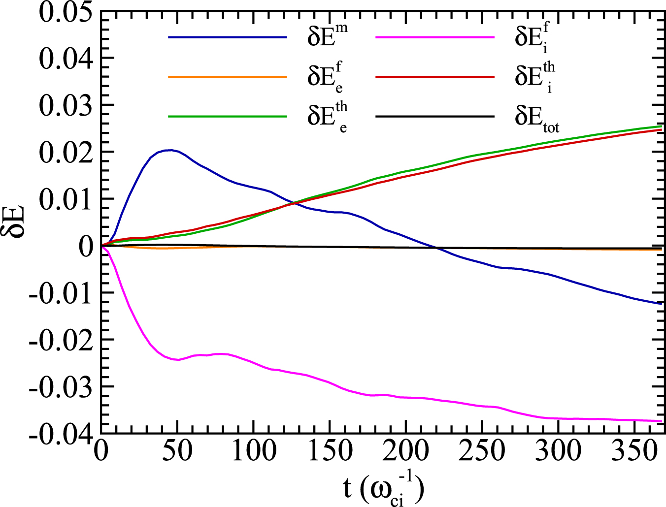
Figure 1 shows the global energy balance by tracking time evolution of the electromagnetic energy 〈E^m 〉, the fluid flow energy of each species $\langle {E}_{\alpha }^{f}\rangle$, and the internal energy of each species $\langle {E}_{\alpha }^{\mathrm{th}}\rangle$. The total energy $\langle {E}_{{tot}}\rangle =\langle {E}^{m}+{E}_{i}^{f}+{E}_{e}^{f}+{E}_{i}^{\mathrm{th}}+{E}_{e}^{\mathrm{th}}\rangle$ is well conserved, indicating the validity of this simulation. Note that the electrons gain slightly more internal energy compared to the ions. The stronger electron energization is in conflict with the findings of Cranmer et al. (2009), Bandyopadhyay et al. (2020a), and Hughes et al. (2014), which all favor stronger ion heating; note that this is consistent with what was observed in Bandyopadhyay et al. (2021), who found stronger electron heating in turbulent magnetic reconnection. As suggested in early studies, the partitioning of heating between ions and electrons depends on turbulence amplitude (Wu et al. 2013; Matthaeus et al. 2016; Hughes et al. 2017) and plasma β (Howes 2010; Vech et al. 2017; Parashar et al. 2018).

Zoom In Zoom Out Reset image size

From Equations (1)–(3), two pathways, the electric work 〈 j _α · E 〉 and the pressure–strain interaction $\langle -\left({{\boldsymbol{P}}}_{\alpha }\cdot {\rm{\nabla }}\right)\cdot {{\boldsymbol{u}}}_{\alpha }\rangle$, contribute to the global energy exchange between forms. Their time histories are shown in Figure 2. One can observe that the global average of the electric work of each species 〈 j _α · E 〉 in Figures 2(a) and (b) oscillates significantly over time at high frequencies. This is likely an artifact of the artificial value of ω_pe /ω_ce in our simulation, and may be remedied by time averaging the results over a plasma oscillation period (Haggerty et al. 2017). The global average of the pressure dilatation of each species p θ_α in Figures 2(c) and (d) also exhibits oscillations, which is attributable to the compression arising from acoustic waves. Since the run we use here is weakly compressible, the incompressive channel PiD_α is favored obviously over the compressive channel p θ_α for both ions and electrons. Therefore, the global average of the pressure–strain interaction of each species $\langle -\left({{\boldsymbol{P}}}_{\alpha }\cdot {\rm{\nabla }}\right)\cdot {{\boldsymbol{u}}}_{\alpha }\rangle$ mainly results from the incompressive part PiD_α . However, we cannot rule out the possibility of stronger p θ_α at some locations. For example, as shown in the magnetosheath (Chasapis et al. 2018b), the turbulent current sheet (Pezzi et al. 2021; Bandyopadhyay et al. 2021) and the electron diffusion region (Zhou et al. 2021), the local compressive part could dominate over the local incompressible part. Note that there is one peak with magnitude much larger than the others in the beginning at $t({\omega }_{{ci}}^{-1})=4.5$. This is due to the initial negligible electric field, which responds quickly to obey a solution of the Vlasov–Maxwell system.

Zoom In Zoom Out Reset image size

Global energy balance in Equations (1)–(3) is shown in Figure 3, where the changes of energies contrast with the cumulative time-integrated pathways. These integrals have been numerically computed through the trapezoidal rule and over time inteval $[9,\,t]({\omega }_{{ci}}^{-1})$ to avoid the effect of the peaks at $t({\omega }_{{ci}}^{-1})=4.5$ shown in Figure 2. According to Equation (2), the internal energy variation of species α, $\delta {E}_{\alpha }^{\mathrm{th}}$, should be equal to the cumulative integral of $\langle -\left({{\boldsymbol{P}}}_{\alpha }\cdot {\rm{\nabla }}\right)\cdot {{\boldsymbol{u}}}_{\alpha }\rangle$, which is confirmed in Figure 3. One can see that the cumulative time integrated $\langle -\left({{\boldsymbol{P}}}_{\alpha }\cdot {\rm{\nabla }}\right)\cdot {{\boldsymbol{u}}}_{\alpha }\rangle$ is almost superposed on the change of internal energy for both electrons and ions. The slight difference mainly results from the level of accuracy of the energy conservation recovered in the simulation and the numerical error of time integration.

Zoom In Zoom Out Reset image size

As expected from Equation (3), the cumulative time integrated 〈− j · E 〉 is in good agreement with the change of the electromagnetic energy, δ E^m . This adds evidence to the idea that despite being adopted widely to estimate heating rate, the electric work 〈 j · E 〉 is not in direct association with either the internal energy increase or the temperature enhancement. Instead, the change of the internal energy takes place directly through the pressure–strain interaction, $\langle -\left({{\boldsymbol{P}}}_{\alpha }\cdot {\rm{\nabla }}\right)\cdot {{\boldsymbol{u}}}_{\alpha }\rangle$, for both ions and electrons.

Further examining Figure 3, we see that the change of the fluid flow energy $\delta {E}_{\alpha }^{f}$ shows similar trends to the cumulative $\langle {{\boldsymbol{j}}}_{\alpha }\cdot {\boldsymbol{E}}+\left({{\boldsymbol{P}}}_{\alpha }\cdot {\rm{\nabla }}\right)\cdot {{\boldsymbol{u}}}_{\alpha }\rangle$, in accordance with Equation (1). The nonnegligible offsets of the two curves arise in large part from the cumulative numerical error associated with the high-frequency oscillations in 〈 j _α · E 〉 shown in Figure 2.

The preceding section investigates global properties of energy conversion in detail. Another important property of plasma turbulence is that it encompasses a vast range of scales. Therefore justification for the identification of relevant dissipation proxies at different scales is crucial. Two simple but essential approaches to resolve or decompose turbulent fields over varying scales are the scale-filtering technique, and structure function technique, which give rise to Equations (7) and (9), respectively.

To proceed numerically using Equation (9), the term ∂_t S(ℓ)/4 is computed by $\left(S({\ell },t+{\rm{\Delta }}t)-S({\ell },t)\right)/{\rm{\Delta }}t$. The gradient ∇_ℓ is computed in lag (ℓ_x , ℓ_y ) space spanning [0, 75d_i ] × [0, 75d_i ] with 256² mesh points in the 2.5D case, and in lag (ℓ_x , ℓ_y , ℓ_z ) space spanning [0, 21d_i ] × [0, 21d_i ] × [0, 21d_i ] with 64³ mesh points in the 3D case. To extract the lag length dependence, we apply directional averaging to obtain lag-length-dependent versions of the quantities T_s , F_s , and D_s .

The analysis procedure selects a time shortly after the mean square current density reaches its maximum, by which time the turbulence is fully established. We use four time snapshots (i.e., $t=97.5{\omega }_{{ci}}^{-1},\,102.5{\omega }_{{ci}}^{-1},\,107{\omega }_{{ci}}^{-1},\,111.5{\omega }_{{ci}}^{-1}$) in the 2.5D case and two time snapshots (i.e., $t=45{\omega }_{{ci}}^{-1},\,50{\omega }_{{ci}}^{-1}$) in the 3D case. These snapshots are separated by time lag ${\rm{\Delta }}t\sim 5{\omega }_{{ci}}^{-1}$. All of the following results are averaged over these time snapshots. Figure 4 shows magnetic energy spectra for the 2.5D case at $t=97.5{\omega }_{{ci}}^{-1}$ and the 3D case at $t=45{\omega }_{{ci}}^{-1}$, where k^−5/3 and k^−8/3 power laws are shown for reference in the range k < 1/d_i and 1/d_i < k < 1/d_e , respectively.

Zoom In Zoom Out Reset image size

In comparison to the 2.5D simulation, the setup of the 3D kinetic simulation is less than optimal, for example, in its relatively small domain size. The expectation follows that, for the 3D case, the interval of MHD inertial scales will be more limited and not well separated from the injection scale. The spectra are characterized with an upturn at high wavenumbers, which is a cumulative effect of the discrete particle noise inherent in the PIC algorithm. Prior to analysis, we remove noise by low-pass Fourier filter with a cutoff at kd_i ∼ 13 for the 2.5D case and kd_i ∼ 21 for the 3D case. This corresponds to filter scales ℓ = π/k ∼ 0.25d_i and ℓ ∼ 0.15d_i , respectively. This filtering procedure has a negligible effect on the following results at scales larger than the cutoff.

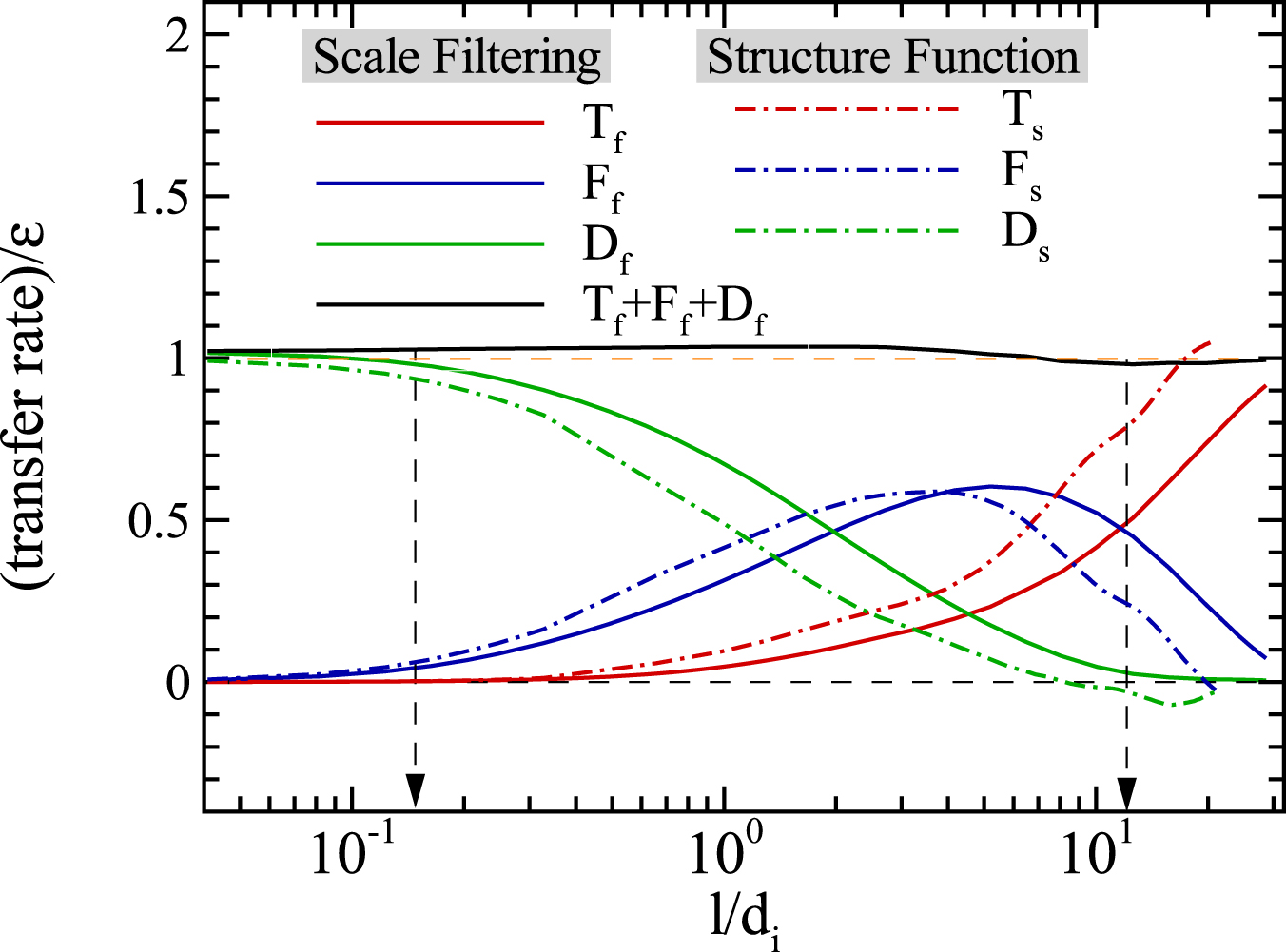
Analysis of the 2.5D case begins with a scale-filtering description of energy balance in Equation (7), shown in Figure 5. The filter cutoff is ℓ = 0.25d_i ∼ d_e , and the correlation length is ℓ ∼ 14d_i , which are indicated by arrows in Figure 5. The k^−5/3 power-law spectrum in Figure 4(a) gives a rough suggestion of an MHD inertial range, in the vicinity of a few d_i . One can see that the time derivative term T_f , which is the time-rate-of-change of the cumulative energy in fluctuations at scales < ℓ, reaches the total dissipation rate at scales larger than the correlation length, and decreases at intermediate scales (roughly the MHD inertial range), where the nonlinear transfer term F_f sets in and reaches a peak value. The plateau (or, peak) of F_f deviates slightly from due to the onset of the pressure–strain interaction D_f , which is not negligible at the scale of peak F_f , and which increases toward at scales much smaller than d_i .

Zoom In Zoom Out Reset image size

A similar balance holds for the structure function representation in Equation (9). In this case, the dissipative term D_s , important at small scales, is computed through ${D}_{\mu }+{D}_{\eta }=\epsilon +{\partial }_{t}S/4+{{\rm{\nabla }}}_{{\boldsymbol{r}}}\cdot \left({\boldsymbol{Y}}/4+{\boldsymbol{H}}/8\right)$. Again, the Yaglom flux F_s , representing energy transfer by turbulence, reaches a plateau over the intermediate (inertial) scales, at values approaching the system dissipation rate . The time derivative term T_s saturates to ∼ at very large scales.

From Figure 5, we observe the following. First, the scale-by-scale energy budget equation in terms of structure functions (Equation (9)), although shifted slightly, is in good agreement with the analogous expressions in terms of scale filters (Equation (7)). Second, the analogy that exists between the filtered pressure–strain interaction D_f and the dissipative term D_s lends credence to the association of the pressure–strain interaction with the dissipation rate. Finally, the energy loss at energy-containing scales equals the nonlinear energy flux at MHD inertial range and the energy dissipated at kinetic scales. Such a well-distinguished range of scales is indicative of a well-separated inertial range. Accordingly, for cases such as this one, the energy decay rates estimated by the von Kármán decay law in Equation (10) and the inertial range energy rate estimated by the Yaglom relation in Equation (11) are reliable proxies of energy dissipation rate.

All systems do not necessarily realize a well-defined scale separation as seen in the 2.5D case shown above; see, for example, the observational result in Chhiber et al. (2018) and Bandyopadhyay et al. (2020). We use the 3D PIC run, in which scale separation is less well defined, to show how the balance of terms appears in Figure 6. Most of points made in Figure 5 remain applicable in Figure 6, such as the analogy between the scale-filtering and structure function representations, and the similarity between the pressure–strain interaction and viscous-resistive effect. In the 3D case (Figure 6), the dissipation rate is well accounted for by the pressure–strain interaction at kinetic scales and by the time-rate-of-change of filtered energy at energy-containing scales. However, both the nonlinear transfer term F_f and the Yaglom flux F_s saturate to values significantly below . This is evidently due to the fact that neither the dissipation D_f (D_s ) nor the time dependence T_f (T_s ) are negligible at those scales.

Zoom In Zoom Out Reset image size

To obtain a "pure" Yaglom relation (Equation (11)), one requires the existence of the MHD inertial range, in which the dynamics is dominated by inertia terms. It is therefore necessary that the MHD inertial range of scales is (i) at scales small enough that the time-rate-of-change of energy at that scale is negligible, and (ii) at scales large enough that the dissipation at that scale can be neglected. In this sense, the 3D case shown in Figure 6 manifestly lacks a well-defined scale separation or a well-separated MHD inertial range. This is consistent with the spectrum in Figure 4(b), but is actually more dramatically illustrated in the analysis shown in the scale decomposition shown in Figure 6. Consequently, in this 3D case, the estimation of dissipation rate based on the Yaglom relation (Equation (11)) falls well below the correct one. Unlike the Yaglom relation, the pressure–strain interaction term traces the conversion of fluid flow energy into internal energy directly, and provides an accurate dissipation rate estimation even in the absence of a well-defined MHD inertial range, as seen in Figures 5 and 6.

As shown in Figure 2, the compressible part p θ_α accounts for a very small fraction of the pressure–strain interaction $\langle -\left({{\boldsymbol{P}}}_{\alpha }\cdot {\rm{\nabla }}\right)\cdot {{\boldsymbol{u}}}_{\alpha }\rangle$ for ions and electrons. In Figure 7, we show how the compressible ${\overline{p\theta }}_{i}+{\overline{p\theta }}_{e}$ and incompressible ${\overline{{PiD}}}_{i}+{\overline{{PiD}}}_{e}$ parts in Equation (8) vary with scales. One can see that the compressible part across scales saturates at kinetic scales, but it is much smaller than the incompressible part for both 2.5D and 3D cases. The compressible part ${\overline{p\theta }}_{i}+{\overline{p\theta }}_{e}$ for the 3D case is negative, while that for the 2.5D case is positive. One explanation for this sign difference is the oscillatory character of p θ_α seen in Figure 2 due to the involvement of acoustic waves.

Zoom In Zoom Out Reset image size

The dissipative mechanism in weakly collisional plasma is a topic that pervades decades of studies without a consensus solution. A number of dissipation proxies are relevant to the turbulence energy transfer process. In this paper, we study the pressure–strain interaction $-\left({{\boldsymbol{P}}}_{\alpha }\cdot {\rm{\nabla }}\right)\cdot {{\boldsymbol{u}}}_{\alpha }$ versus other proxies, such as the electromagnetic work j · E , the energy decay rate _vk from the von Kármán decay law (Wan et al. 2012b; Wu et al. 2013; Zank et al. 2017; Bandyopadhyay et al. 2018b, 2019), and the energy transfer rate _Ym from the Yaglom relation (Politano & Pouquet 1998; Sorriso-Valvo et al. 2007; Stawarz et al. 2009; Coburn et al. 2015; Verdini et al. 2015; Bandyopadhyay et al. 2018a). Both the global energy balance and energy budget across scales using the scale-filtering and structure function representations ⁷ are investigated here in detail in 2.5D and 3D kinetic simulations. We argue here that the pressure-strain interactions are exact representations of energy dissipation defined as conversion into internal energy; for a more complete review of various approximate dissipation proxies, see Pezzi et al. (2021).

We confirm that although the electromagnetic work j · E has been widely used, the change of the internal energy of each species take places directly through the pressure–strain interaction $-\left({{\boldsymbol{P}}}_{\alpha }\cdot {\rm{\nabla }}\right)\cdot {{\boldsymbol{u}}}_{\alpha }$. In comparison with the electric work j · E , the pressure–strain interaction $-\left({{\boldsymbol{P}}}_{\alpha }\cdot {\rm{\nabla }}\right)\cdot {{\boldsymbol{u}}}_{\alpha }$ has the advantage of tracking electron and ion heating separately. Meanwhile, there can be a correlation between the electromagnetic work and the pressure–strain interaction. For example, from a generalized Ohm's law or the electron momentum equation, in the limit of massless electrons, we can find that $\langle {{\boldsymbol{j}}}_{e}\cdot {\boldsymbol{E}}\rangle =\langle -\left({{\boldsymbol{P}}}_{e}\cdot {\rm{\nabla }}\right)\cdot {{\boldsymbol{u}}}_{e}\rangle$. No such relation can be obtained for protons.

The detailed treatment of energy transfer across scales using the scale-filtering and structure function representations demonstrates significant caveats pertinent to typical estimations of dissipation based on the von Kármán decay law and the Yaglom relation, while the same analysis shows the advantages of the pressure–strain interaction $\langle -\left({{\boldsymbol{P}}}_{\alpha }\cdot {\rm{\nabla }}\right)\cdot {{\boldsymbol{u}}}_{\alpha }\rangle$ over other proxies to estimating energy dissipation rate. At energy-containing scales, the time-rate-of-change of energy can be taken as the dissipation rate. However, in real data environment from observations, due to the infeasibility of obtaining the time derivative term, we resort to the von Kármán decay law (Equation (10)) to compute the energy decay rate. This may be inaccurate due to uncertainty of the choices for the similarity lengths L_± and the von Kármán constants α_±.

In the MHD inertial range of scales, existing studies of energy dissipation in kinetic plasmas have had a particular leaning toward use of the Yaglom relation in observations and simulations, with only rare attempts made to circumscribe its domain of validity. While we are aware of the important recent developments in deriving Yaglom-like relations for compressible MHD, we have not opted in the present study to implement these theories due to their general complexity, variety of forms, and specialization (in some cases) to isothermal turbulence. The incompressive form that we use here evidently remains relevant to our weakly compressible kinetic simulations. Our 2.5D kinetic simulation exhibits a range of scales (inertial range) over which the inertial range energy transfer rate from the Yaglom relation fits well with the real dissipation rate, while an observably underestimated inertial range energy transfer rate emerges in our 3D case. This is attributable to the lack of a well-separated inertial range in the 3D kinetic simulation used here. It is worth emphasizing that the Yaglom relation requires that there exists a well-separated inertial range, but a well-defined scale separation is not guaranteed a priori.

As suggested in Antonia & Burattini (2006) and Ferrand et al. (2022), a finite Reynolds number and the nonstationarity or inhomogeneity associated with large scales can affect the behavior of the scales in the inertial range significantly. In general, a substantial inertial range is more likely to be established when the Reynolds number is large and forcing is applied. One may also note that even though the decaying turbulent flows used here introduce the time nonstationarity, the Yaglom relation remains valid within the inertial range for the 2.5D kinetic simulation (Ferrand et al. 2022), provided that the system is sufficiently large, i.e., characterized by large effective Reynolds number (Parashar et al. 2015). It is worth pointing out that there are no universal conditions under which the Yaglom relation is guaranteed to be valid.

Reconsideration of the assumptions necessary to arrive at the Yaglom relation casts doubt on its widespread use to estimating the dissipation rate in collisionless plasmas. First, even though the turbulence normally encountered in most of space plasmas (e.g., the solar wind and the magnetosheath) is very well developed, specific instances do not necessarily realize a well-defined scale separation. See, for example, the observational result in Chhiber et al. (2018) and Bandyopadhyay et al. (2020). Consequently, the prediction that follows from the Yaglom relation should be questioned in all cases absent a well-defined inertial range. Second, the Yaglom flux _Ym in Equation (11) requires accurate determination of derivatives in 3D lag space, which is, in general, inaccessible in observational or experimental situations. Consequently, a simplified form derived assuming isotropy (Politano & Pouquet 1998) is often used for solar wind and magnetosheath turbulence that is anisotropic. One can imagine the limitations of such approaches when strong anistropy exists, but the opportunities for suitable direction averaging (Taylor et al. 2003) are limited. We intend to further explore direction averaging in a subsequent publication.

In contrast, the pressure–strain interaction $\langle -\left({{\boldsymbol{P}}}_{\alpha }\cdot {\rm{\nabla }}\right)\cdot {{\boldsymbol{u}}}_{\alpha }\rangle$ without requiring isotropy turns out to be an accurate estimation of the real dissipation rate even in the absence of a well-defined inertial range. The pressure–strain interaction dominates at kinetic scales d_e , so that deep in the dissipation range, all dissipation is accounted for. One may note that the pressure–strain interaction is also analogous to the viscous-collisional case in the sense that its global average could depend on velocity gradient as well (Vasquez & Markovskii 2012; Yang et al. 2017a; Del Sarto & Pegoraro 2018; Parashar et al. 2018).

In principle, the pressure–strain interaction $\langle -\left({{\boldsymbol{P}}}_{\alpha }\cdot {\rm{\nabla }}\right)\cdot {{\boldsymbol{u}}}_{\alpha }\rangle$ is a much more complete representation of dissipation in kinetic plasma in several ways. First, $\langle -\left({{\boldsymbol{P}}}_{\alpha }\cdot {\rm{\nabla }}\right)\cdot {{\boldsymbol{u}}}_{\alpha }\rangle$ is readily resolved into contributions of electrons and ions (and additional species if present). Therefore this approach is useful to understand the distribution of dissipated energy between different species (Sitnov et al. 2018; Bandyopadhyay et al. 2021). Second, $\langle -\left({{\boldsymbol{P}}}_{\alpha }\cdot {\rm{\nabla }}\right)\cdot {{\boldsymbol{u}}}_{\alpha }\rangle$ includes both compressive and incompressive contributions, while most of the other estimates are limited to incompressive contributions. The kinetic simulations used here are weakly compressive, and more samples with stronger compression are required to assess detailed contributions from the compressive part of $\langle -\left({{\boldsymbol{P}}}_{\alpha }\cdot {\rm{\nabla }}\right)\cdot {{\boldsymbol{u}}}_{\alpha }\rangle$ to the energy dissipation (Chasapis et al. 2018b; Du et al. 2018; Pezzi et al. 2021; Bandyopadhyay et al. 2021; Wang et al. 2021; Zhou et al. 2021). Third, $\langle -\left({{\boldsymbol{P}}}_{\alpha }\cdot {\rm{\nabla }}\right)\cdot {{\boldsymbol{u}}}_{\alpha }\rangle$ remains applicable to anistropic cases, in which one may identify a preferred direction that influences the nature of dissipation (Song et al. 2020; Bacchini et al. 2022). Finally, without taking a spatial average, $-\left({{\boldsymbol{P}}}_{\alpha }\cdot {\rm{\nabla }}\right)\cdot {{\boldsymbol{u}}}_{\alpha }$ is spatially localized, which can be applied to examine the contribution from each point in space and identify sites of heating (Yang et al. 2017a, 2017b; Pezzi et al. 2019b; Yang et al. 2019). We should also keep in mind that the transport terms shown in Equation (2) are likely to exert significant influence on the values of $-\left({{\boldsymbol{P}}}_{\alpha }\cdot {\rm{\nabla }}\right)\cdot {{\boldsymbol{u}}}_{\alpha }$ (Du et al. 2020; Fadanelli et al. 2021) actually obtained, and may therefore influence observed local temperature increase, even if the pressure–strain remains an accurate quantitative measure of the dissipation itself.

This research has been supported by NSFC grant Nos. 11902138, 91752201, and 11672123, by the US National Science Foundation under NSF-DOE grant PHYS- 2108834, by the NASA Magnetospheric Multiscale mission under NASA grant 80NSSC19K0565, by NSF/DOE grant DE-SC0019315 and XSEDE allocation TG-ATM180015, and by Department of Science and Technology of Guangdong Province (grant No. 2020B1212030001) and Shenzhen Science & Technology Program (grant No. KQTD20180411143441009). We acknowledge computing support provided by Center for Computational Science and Engineering of Southern University of Science and Technology and the use of Information Technologies (IT) resources at the University of Delaware, specifically the high-performance computing resources.