


Abstract
The advent of sensitive gravitational-wave (GW) detectors, coupled with wide-field, high-cadence optical time-domain surveys, raises the possibility of the first joint GW–electromagnetic detections of core-collapse supernovae (CCSNe). For targeted searches of GWs from CCSNe, optical observations can be used to increase the sensitivity of the search by restricting the relevant time interval, defined here as the GW search window (GSW). The extent of the GSW is a critical factor in determining the achievable false alarm probability for a triggered CCSN search. The ability to constrain the GSW from optical observations depends on how early a CCSN is detected, as well as the ability to model the early optical emission. Here we present several approaches to constrain the GSW, ranging in complexity from model-independent analytical fits of the early light curve, model-dependent fits of the rising or entire light curve, and a new data-driven approach using existing well-sampled CCSN light curves from Kepler and the Transiting Exoplanet Survey Satellite. We use these approaches to determine the time of core-collapse and its associated uncertainty (i.e., the GSW). We apply our methods to two Type II SNe that occurred during LIGO/Virgo Observing Run 3: SN 2019fcn and SN 2019ejj (both in the same galaxy at d = 15.7 Mpc). Our approach shortens the duration of the GSW and improves the robustness of the GSW compared to the techniques used in past GW CCSN searches.
Export citation and abstract BibTeX RIS

Original content from this work may be used under the terms of the Creative Commons Attribution 4.0 licence. Any further distribution of this work must maintain attribution to the author(s) and the title of the work, journal citation and DOI.
1. Introduction
Following the detection of gravitational-wave (GW) emission from compact-object binary mergers (Abbott et al. 2016a, 2016c, 2016d, 2017), additional known GW sources yet to be detected are core-collapse SNe (CCSNe), representing the deaths of stars more massive than ≈8 M⊙. While CCSNe are volumetrically much more common than binary mergers, their GW emission is expected to be weaker (Murphy et al. 2009; Müller et al. 2013; Kuroda et al. 2016; Andresen et al. 2017, 2019; Powell & Müller 2019; Radice et al. 2019; Vartanyan et al. 2019), and they are thus likely to be detectable in a much more limited volume.
Still, the GW detection of CCSNe will provide a critical view of the core-collapse process itself, which is not directly accessible through electromagnetic (EM) observations. In particular, since GW emission is produced by the quadrupole distribution of energy and mass, it can probe the degree of asymmetry and angular momentum in the core-collapse process (Foglizzo et al. 2009; Janka et al. 2012, 2016; Vartanyan et al. 2019).
GW detections of CCSNe present distinct challenges compared to detections of binary mergers, which have well-defined waveforms that enable a search based on template matching (Babak et al. 2006; van den Broeck et al. 2009; Usman et al. 2016; Roulet et al. 2019; Roy et al. 2019). Although there are some critical GW features in time–frequency space that carry imprints of the underlying core-collapse physics, the nature of the waveforms is expected to be predominantly stochastic (Janka 2012; Janka et al. 2016; Kuroda et al. 2016; Andresen et al. 2017, 2019; Hayama et al. 2018; Kawahara et al. 2018; O'Connor & Couch 2018; Takiwaki & Kotake 2018; Powell & Müller 2019; Radice et al. 2019; Vartanyan et al. 2019). Moreover, the energy conversion in GWs is expected to vary, depending on the progenitor and the details of the explosion mechanism (Kotake et al. 2009; Marek et al. 2009; Murphy et al. 2009; Ott 2009; Scheidegger et al. 2010; Yakunin et al. 2010, 2015; Kuroda et al. 2012, 2016, 2017; Ott et al. 2012, 2013; Couch 2013; Hanke et al. 2013; Kotake 2013; Müller et al. 2013; Nakamura et al. 2014; Abdikamalov et al. 2015; Hayama et al. 2015; Andresen et al. 2017, 2019; Sotani et al. 2017; Hayama et al. 2018; Kawahara et al. 2018; Morozova et al. 2018; Takiwaki & Kotake 2018; Radice et al. 2019).
Even the most favorable core-collapse GW emission models point to a detection horizon that does not extend much beyond the local universe (D ≲ 25 Mpc). For current generic GW burst searches at the design sensitivity of Advanced LIGO/Virgo for slowly rotating progenitors, only CCSNe within the Galaxy are expected to be detectable (Acernese et al. 2015; Abbott et al. 2016b, 2020; Szczepańczyk et al. 2021). The rate of CCSNe is about 1 in 50 yr in the Galaxy, and it grows to a few per year within a few Mpc (van den Bergh et al. 1987; van den Bergh & Tammann 1991; Cappellaro et al. 1993, 1997, 1999, 2015; Tammann et al. 1994; Karachentsev et al. 2004; Ando et al. 2005; Li et al. 2011; Botticella et al. 2012; Dahlen et al. 2012; Mattila et al. 2012; Rozwadowska et al. 2021).
Given the expected complexity of the GW signal, and the limited detection range, it is essential to use all avenues to improve the chances of detection. These include detector hardware improvements, the continued development of reliable core-collapse simulations, the inclusion of progenitor properties as inputs to detection algorithms, and the use of optical data for the purpose of pinpointing the location and distance, as well as for minimizing the GW search window (GSW). Here, we specifically focus on the latter point. Estimating the GSW depends on two steps: (i) determining the time delay between core collapse and the start of optical emission (shock breakout; SBO), Δtcc ≡ tSBO − tcc; and (ii) determining the time of SBO, tSBO, using available optical data. We explore several approaches for the latter, and use the results of numerical simulations for the former (Barker et al. 2021). By way of example, we apply our methodology to Type II SNe that occurred during LIGO/Virgo Observing Run 3, with the specific requirements of: (i) a distance of ≲20 Mpc (to have a nonzero GW detection efficiency); and (ii) sufficient optical data to constrain the GSW to ≲week in order to improve the search sensitivity and statistical confidence relative to an unconstrained search (Abadie et al. 2010; Lynch & LIGO/Virgo Collaboration 2018; Abbott et al. 2019). Two CCSNe that match these requirements 5 are SN 2019fcn and SN 2019ejj.
The paper is organized as follows. In Section 2, we present the two CCSNe and our analysis of their available photometry and spectroscopy. In Section 3, we briefly review the existing methodology of calculating the GSW as used by the LIGO/Virgo Collaboration (LVC). In Section 4, we introduce four new methodologies to more robustly estimate the time of SBO from the SN data, and we use theoretical models to estimate the delay between core collapse and SBO. In Section 5, we present the results of these methodologies as applied to the two CCSNe considered here. We discuss the implications of these results in Section 6 and conclude in Section 7.
2. Discovery and Observations of SN 2019ejj and SN 2019fcn
SN 2019ejj was discovered by the Asteroid Terrestrial-impact Last Alert System on 2019 May 2.26 UT (2458605.76; Nicholl et al. 2019b) and classified as a Type II SN by the extended Public ESO Spectroscopic Survey for Transient Objects (ePESSTO) with a spectrum taken on 2019 May 2.98 (Nicholl et al. 2019b). SN 2019fcn was discovered by the All-Sky Automated Survey for Supernovae on 2019 May 5.96 (Stanek et al. 2019) and classified as a Type II SN by ePESSTO with a spectrum taken on 2019 May 14.03 (2458612.46; Nicholl et al. 2019a). Both of these SNe exploded within a few days of each other in the same galaxy, ESO 430-G 020, which has a Tully–Fisher distance of ≈15.7 Mpc (Theureau et al. 2007).
Both SNe 2019ejj and 2019fcn were observed in the UBVgri filters with the Las Cumbres Observatory's global network of 1 m telescopes, equipped with Sinistro cameras (Brown et al. 2013), as part of the Global Supernova Project. Because SN 2019fcn exploded in the same galaxy as SN 2019ejj, we serendipitously observed SN 2019fcn on 2019 May 5.06, at 21.7 hr (2458611.57), before it was discovered by ASAS-SN. We treat this earlier observation as the discovery in the following analysis.
We subtracted BVgri reference images, also taken with a Sinistro camera, on 2020 March 8, after both SNe had faded, from the earlier observations using PyZOGY (Guevel & Hosseinzadeh 2017), a Python implementation of the image subtraction algorithm of Zackay et al. (2016). We extracted point-spread function photometry using lcogtsnpipe (Valenti et al. 2016), and calibrated the photometry relative to the Pan-STARRS1 3π catalog (Chambers et al. 2016). For B and V, we transformed the catalog magnitudes according to Lupton (2005).
We corrected the resulting magnitudes for Galactic extinction using the dust maps of Schlafly & Finkbeiner (2011) and the extinction law of Cardelli et al. (1989). We note that there is relatively high Galactic extinction in the direction of ESO 430-G 020, with AV = 1.22 mag. This, combined with the galaxy's low redshift, makes it difficult to discern whether either of these SNe suffer from additional host galaxy extinction. Our spectra of SN 2019fcn show very strong (Wλ ≈ 0.29 nm) Na iD absorption at z = 0. This is beyond the regime where equivalent width correlates with dust extinction. Given the large Galactic extinction, we assume that any host galaxy extinction is small in comparison. Finally, we converted to absolute magnitudes using the Tully–Fisher-based distance modulus μ = 31.0 ±0.4 mag (Theureau et al. 2007). The photometry is available as the data behind Figure 9.
We also obtained two spectra of SN 2019ejj and four spectra of SN 2019fcn with the FLOYDS spectrographs on the Las Cumbres Observatory's 2 m telescopes (Brown et al. 2013), using a 2'' slit oriented at the parallactic angle, and reduced them using the floydsspec pipeline (Valenti et al. 2014). These spectra are available from the Weizmann Interactive Supernova Data Repository (Yaron & Gal-Yam 2012).
3. Calculating the GSW Using the LVC Early Observation Method (EOM)
Abbott et al. (2020, hereafter LVC20) calculate the GSW (referred to as the on-source window) using the Early Observation Method (EOM) for four CCSN candidates. The EOM defines the GSW as the time range between t1 = tnd − ΔtSB and t2 = tfd, where tfd is the time of the first optical detection, tnd is the time of the last observation without the SN present, and ΔtSB accounts for the shock propagation travel time between core collapse and SBO; LVC20 employ a range of 15–24 hr for the latter (Schawinski et al. 2008; Dessart et al. 2017) to account for the unknown progenitor star properties. However, when reporting the on-source windows, LVC20 actually use a fixed ΔtSB =15 hr. A schematic view of the EOM from LVC20 is shown in Figure 1.
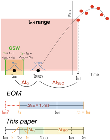
Figure 1. Top: a schematic view of how to calculate the GSW (yellow shaded region) from a supernova optical light curve (red points; Hicken et al. 2017). We constrain the GSW by fitting the light curve with several models to determine tSBO, and then use theoretical estimates to determine tcc. Middle: the EOM approach adopted by LVC20 uses the first optical detection (tfd) and previous nondetection (including a fixed SBO timescale: tnd − 15 hr) to determine the GSW. Depending on the details of the optical data, the EOM may actually miss tcc. Bottom: our approach avoids the pitfalls of the EOM by not strictly depending on specific data points, but instead considers the rising part or the full optical light curve to directly fit for ΔtSBO. For Δtcc, we use a much wider range of possible values to account for progenitor uncertainties.
Download figure:
Standard image High-resolution imageThe EOM approach suffers from four potential shortcomings. First, it assumes that the time of core collapse (tcc), and hence GW emission, is bracketed by t1 and t2, but this cannot be guaranteed as it depends critically on the relative sensitivity of the nondetection at tnd compared to the brightness of the SN at tfd. Second, allowing the GSW to extend all the way to tfd makes the GSW too wide, since clearly tcc cannot be at tfd. Third, since optical time-domain surveys have a range of cadences and sensitivities, and are further affected by weather, it is possible that the time interval between t1 and t2 will in fact contain tcc, but will be much wider than necessary. Fourth, existing studies (Chevalier 1992; Matzner & McKee 1998; Calzavara & Matzner 2004; Chevalier & Irwin 2011; Kistler et al. 2013; Morozova et al. 2015; Davies 2017; Müller et al. 2017; Waxman & Katz 2017; Barker et al. 2021) suggest a much wider range for ΔtSB than the single value of 15 hr used by LVC20. Thus, depending on the specific circumstances of each CCSN, the GSW (as defined by the EOM) may actually miss the time of GW emission, or alternatively may be much wider than needed.
It is also worth pointing out that the GSWs reported in this paper might not also reach 100% probability of including GW emission. We discuss this limitation in regards to the EOM and point out how to eliminate three of the drawbacks and mitigate the fourth one in this paper. However, the point of any targeted GW search is not to maximize the detection probability to 100%, but to increase the overall probability of detection for a larger fraction of GW candidates. This line of operation has also been used in previous GW searches as part of the tuning methodologies.
For the purpose of comparison with the EOM implementation of LVC20, in Table 1 we list the resulting GSW set by the EOM for the two SNe considered here. The left column (LVC20 EOM) uses t1 = tnd − 15 hr and t2 = tfd. The middle column (Corrected LVC20 EOM) applies an additional shift to the GSW (to correctly account for ΔtSB as defined by Abbott et al. 2020) using t1,1 = tnd − 24 hr and t2,2 = tfd − 15 hr. In the right column (Updated EOM), we use updated SBO delay estimates based on the recent work of Barker et al. (2021; their Figure 6) and the observed range of Type IIP SN progenitors in the local universe (see Section 4.2). The updated EOM defines t1,updated = tnd − 3 days and t2,updated = tfd − 1.4 days. In the context of the EOM approach, we consider this latter estimate to be the most robust.
Table 1. GSW Using the EOM
| LVC20 EOM | Corrected LVC20 EOM | Updated EOM | |||||||
|---|---|---|---|---|---|---|---|---|---|
| CCSN | t1 | t2 | GSW | t1,1 | t2,2 | GSW | t1,updated | t2,updated | GSW |
| (JD) | (days) | (JD) | (days) | (JD) | (days) | ||||
| SN 2019ejj | 2458599.16 | 2458605.76 | 6.60 | 2458598.78 | 2458605.13 | 6.35 | 2458596.78 | 2458604.36 | 7.58 |
| SN 2019fcn | 2458608.89 | 2458612.46 | 3.57 | 2458608.52 | 2458611.84 | 3.32 | 2458606.52 | 2458611.06 | 4.54 |
Note. Determinations of the GSW for SNe 2019ejj and 2019fcn using the EOM method. Left: t1 = tnd − 15 hr and t2 = tfd. Middle: t1,1 = tnd − 24 hr and t2,2 = tfd − 15 hr. Right: t1,updated = tnd − 3 days and t2,updated = tfd − 1.4 days. Here, tfd is the first optical detection of an SN and tnd is its previous nondetection. Our updated EOM is more robust and realistic than the one from LVC20.
Download table as: ASCIITypeset image
Table 2. Model Parameters for the Methods Used to Calculate ΔtSBO
| Method | Input Data | Parameters |
|---|---|---|
| Quadratic | Early Photometry | ΔtSBO, α, β |
| Shock-cooling | Early Photometry | ΔtSBO, vs*, Menv, R, M, fρ |
| Empirical Fits | Early Photometry | ΔtSBO, η, 
|
| PP15 | Entire Photometry and Spectroscopy | t0 ≡ ΔtSBO, tP , tw , E(B − V), ω, μ |
Note. A description of the parameters is given in Section 4.
Download table as: ASCIITypeset image
4. New Methods for Calculating the GSW
The EOM approach described in the previous section, including our updates to the LVC calculation, does not make use of all of the available information from optical SN data and modeling. In this section, we introduce and explore several methods for better determining the GSW (with the methods and their associated parameters being described via Table 2). As illustrated in Figure 1, estimating the GSW requires a determination of both ΔtSBO = tfd − tSBO and Δtcc = tSBO − tcc, and their associated uncertainties.
4.1. Estimating the Time to SBO and ΔtSBO
In this paper, we model either the early SN light curves (i.e., the rise to peak) or the full light curves to determine tSBO and its associated uncertainty. Our general approach is shown schematically in Figure 1. We define zero time as the time of first detection (tfd). We use four different approaches, with varying levels of assumptions and complexity: (i) a simple quadratic polynomial fit, which we assume for the early rise of the SN light curve and does not assume any specific physics; (ii) an analytical shock-cooling model, based on the formulation of Sapir & Waxman (2017); (iii) a novel data-driven approach, in which we use high-cadence early light curves of Type II SNe observed with Kepler (Garnavich et al. 2016) and the Transiting Exoplanet Survey Satellite (TESS; Vallely et al. 2021) as input models; and (iv) using the full data set of photometry and spectroscopy to model the entire light curve using the method of Pejcha & Prieto (2015a, 2015b). We describe each method in detail below.
4.1.1. Quadratic Polynomial Fit
The rising phase of SNe empirically follows a low-order polynomial, so here we fit the early photometry with a quadratic polynomial of the form 6

where tSBO is the time of first light (i.e., zero flux) measured in days, and α and β are polynomial coefficients. We use a Markov Chain Monte Carlo (MCMC) routine using pymc3 (Salvatier et al. 2015) to fit for the three free parameters. For α and β, we use a log-uniform prior with a wide range of [−10, 10] to avoid biasing the posterior. For tSBO, we use a uniform prior spanning [−20, 0] days. We also fit for an intrinsic scatter parameter, σ, which we add in quadrature to the observational uncertainties of each data point ( ), with a half-Gaussian prior peaking at 0 and with a standard deviation of 0.1 in units of normalized flux. Figure 2 shows the resulting fits to the optical r-band light curves of SNe 2019fcn and 2019ejj, where the resulting best-fit regions allowed by the data indicate the uncertainty in ΔtSBO.
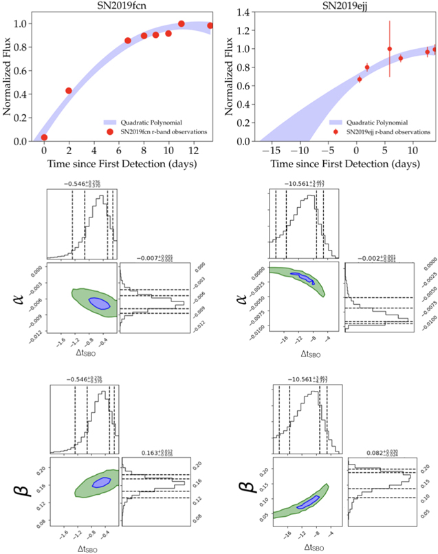
Figure 2. Top panels: second-order polynomial fits (blue curves) to the optical r-band light curves (red points) of SN 2019fcn (left) and SN 2019ejj (right). The intersection of the blue region with zero flux represents the 1σ range on ΔtSBO. As expected, a less-well-sampled early light curve (SN 2019ejj) leads to a larger uncertainty on ΔtSBO. Middle and bottom panels: two-dimensional posterior distributions of ΔtSBO, α, and β for SN 2019fcn (left) and SN 2019ejj (right). The dashed lines in the projected histograms mark the 5%, 16%, 84%, and 95% quantile ranges. The blue and green contours mark the appropriate confidence regions.
Download figure:
Standard image High-resolution image4.1.2. Shock-cooling Model
The early light curves of Type II SN are dominated by shock-cooling emission before hydrogen recombination becomes an important source of heating. We employ the shock-cooling model of Sapir & Waxman (2017), which modeled the expanding and cooling ejecta of a CCSNe following SBO. The model used a red supergiant (RSG) progenitor fit with a broken power-law density profile. The envelope is defined as the mass above the radius at which the density profile steepens. The relevant model parameters of the model are the shock velocity (vs*), envelope mass (Menv), progenitor radius (R), ejecta mass (M), an order-unity factor describing the inner envelope structure (fρ ), and the time of SBO (t0 ≡ tSBO).
We fit this model to the early portion of our multiband light curves using the MCMC routine implemented in the Light Curve Fitting package (Hosseinzadeh & Gomez 2020), including a multiplicative intrinsic scatter term ( ), such that the resulting reduced χ2 ≈ 1 (Andrae et al. 2010). The model holds for temperatures <0.7 eV (8120 K), above which hydrogen recombination effects may be neglected and the approximation of constant opacity holds. As such, we did not fit points below this temperature. Figures 3 and 4 show the results for SNe 2019fcn and 2019ejj, respectively.

Figure 3. Results of the Sapir & Waxman (2017) shock-cooling model fits to the early light curve of SN 2019fcn (top right). The corner plot shows the posterior probability distributions for vs*, Menv, fρ M, R, t0 = tSBO, and σ. The 1σ credible intervals for each parameter, centered on the median, are listed at the top.
Download figure:
Standard image High-resolution image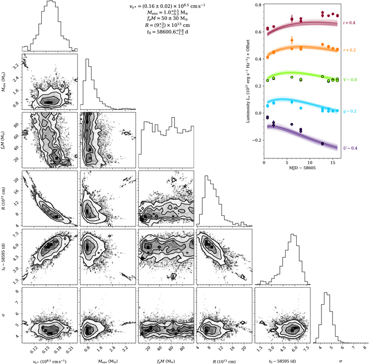
Figure 4. The same as Figure 3, but for SN 2019ejj.
Download figure:
Standard image High-resolution image4.1.3. Empirical Fits Using Kepler and TESS Type II SN Light Curves
Over the past few years, high-cadence observations with Kepler and TESS have led to detailed early light curves of several Type IIP SNe (Garnavich et al. 2016; Vallely et al. 2021). Here we use this library (where naming conventions for the Kepler and TESS SNe are taken from Vallely et al. 2021) of well-measured early light curves to empirically fit for ΔtSBO in SNe 2019ejj and 2019fcn.
From the 14 Type II SNe observed by TESS (Vallely et al. 2021) and the 2 SNe observed by Kepler (Garnavich et al. 2016), we choose the nine highest-quality light curves as empirical templates, discarding events with large scatter. We adopt the tSBO values for these events from Vallely et al. (2021) and Garnavich et al. (2016). We dynamically bin the 3 hr sampled data in intervals spanning 0.3–1 days. We normalize the flux, such that 1 is the peak in the binned flux. We interpolate our templates to the observed times of SNe 2019ejj and 2019fcn during the fit, which applies the stretch in flux and offset in phase, in order to calculate the likelihood for a given model.
We use an MCMC routine in pymc3 (Salvatier et al. 2015) to fit for three free parameters: ΔtSBO, and multiplicative "stretch" factors in phase and flux. The stretch in phase has a log-normal prior centered at 1, with a standard deviation of 0.1 (corresponding to a stretch in phase within 10%), in order to minimize nonphysical and/or artificial distortions to the model light curves. 7 The stretch in flux has a uniform prior centered at 1, spanning [0.5, 2]. For ΔtSBO, we use a uniform prior spanning [−20, 0]. We fit for the intrinsic scatter parameter, σ, as in Section 4.1.1. We apply the fitting to only the r-band data, since it is the closest to the broadband photometry provided by both Kepler and TESS.
In Figures 5 and 6, we show the empirical model light-curve fits, and in Figures 7 and 8 we show the resulting two-dimensional posteriors for ΔtSBO and the stretch in phase, for SNe 2019fcn and 2019ejj, respectively.
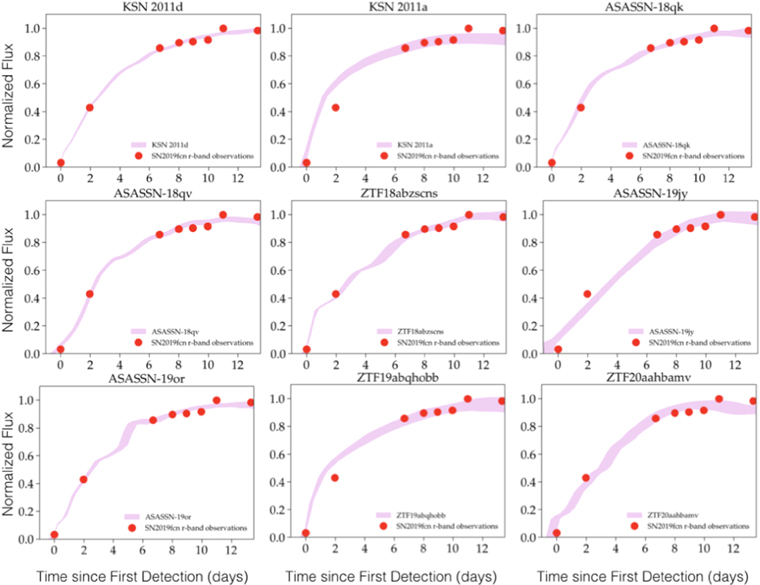
Figure 5. Empirical light-curve fits for SN 2019fcn. The intersection of the pink region with the x-axis represents the 1σ range on tSBO using the empirical light curve templates constructed from Section 4.1.3.
Download figure:
Standard image High-resolution image
Figure 6. The same as Figure 5, but for SN 2019ejj.
Download figure:
Standard image High-resolution image
Figure 7. Two-dimensional posterior distributions of ΔtSBO and the stretch in phase for SN 2019fcn using the empirical Kepler and TESS light curves. The dashed lines in the projected histograms mark the 5%, 16%, 84%, and 95% quantile ranges. The blue and green contours mark the appropriate confidence regions.
Download figure:
Standard image High-resolution image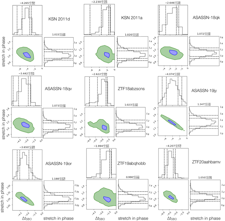
Figure 8. The same as Figure 7, but for SN 2019ejj.
Download figure:
Standard image High-resolution image4.1.4. Pejcha & Prieto (2015) Model
We employ the method of Pejcha & Prieto (2015a, 2015b, hereafter PP15), which uses a combination of photometric and velocity measurements, to provide an estimate of tSBO. This estimate is obtained from fitting the apparent angular radius versus the expansion velocity (obtained through spectroscopic measurements) through the application of the expanding photosphere method (Schmidt et al. 1994; Vinkó & Takáts 2007; Emilio Enriquez et al. 2011; Bose & Kumar 2014).
The velocity measurements fed into the model are obtained by measuring the photospheric velocity as a function of time by fitting the Hα feature in the four individual spectra (i.e., taken at four different epochs) of SN 2019fcn and the two spectra of SN 2019ejj. We use the interactive Spectrum Fitting package (Hosseinzadeh et al. 2020) to define this continuum in time, fit a P Cygni profile, and derive the velocity from the minimum of the absorption.
PP15 also construct a model of the multiband light curves. The multiband light-curve model is dependent on the construction of the spectral energy distribution (SED). We then use the SED to derive both the photospheric radius and temperature variations. The model light curves shown in Figure 9 begin at an estimated tSBO when the optical flux rises due to photospheric expansion and cooling, where the peak of the SED is in the optical bands.
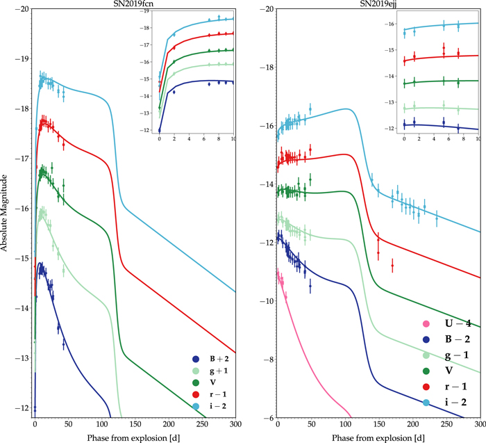
Figure 9. Light-curve model fits for SN 2019fcn (left) and SN 2019ejj (right) using the PP15 model. The insets focus on the early phases of the light curves and show that the model can capture the rising behavior, especially for photometrically well-sampled candidates. The photometry is available as the data behind the figure in the online article.(The data used to create this figure are available.)
Download figure:
Standard image High-resolution imageThe relevant parameters of the model are the total reddening (E(B − V)), the expansion velocity power-law exponent (ω), the plateau duration (tP ), the plateau transition width (tw ), the distance modulus (μ), and the so-called explosion time (t0), which is equivalent to tSBO.
We renormalize the error bars by multiplying them by a factor of 2.70 for SN 2019fcn and a factor of 1.38 for SN 2019ejj in order to reduce χ2 = 1 and account for intrinsic scatter present in the photometric measurements. Figure 9 shows the resulting best-fit models for SNe 2019fcn and 2019ejj using the PP15 method.
4.2. The Delay between Core Collapse and SBO, Δtcc
In the previous section, we addressed the determination of the time of SBO, tSBO. To determine the entire length of the GSW, we also need to include the time delay between core collapse and SBO, Δtcc. This delay is progenitor-dependent, due to the travel time of the SN shock through the progenitor star. Since the progenitor properties are difficult to ascertain in detail, and since there is currently no empirical information on Δtcc, we resort to using theoretical estimates. In particular, we use the recent work of Barker et al. (2021), where estimated ranges for Δtcc are given for a range of zero-age main-sequence masses. We focus on the case of Type II SNe, which arise from RSG stars.
Assuming the progenitor mass is generally ≲20 M⊙ (Negueruela et al. 2016; Davies 2017; Groh 2017; Davies & Beasor 2018), we apply a conservative range of Δtcc ≈ 1.4–3 days, covering the range of masses, as well as theoretical assumptions and uncertainties.
We thus define the GSW by shifting the time window relative to tSBO by this range; namely, we shift and extend the time range defined by tSBO and its associated uncertainty to 3 days earlier from the lower end of the range and 1.4 days earlier from the upper end of the range (see Figure 1, where this shift is applied in the two GSWs resulting from the Updated EOM and the Method from this paper).
We note that for some SNe with well-determined values of tSBO, the theoretical uncertainty in Δtcc may become the dominant source of uncertainty in the GSW. In the absence of firmer constraints on SN shock propagation, and a reliable determination of progenitor properties, we advocate for a more conservative range for Δtcc.
5. Results for SN 2019ejj and SN 2019fcn
In the previous section, we presented several methods for determining ΔtSBO, with increasing model complexity and level of physical accuracy. Here we summarize the results of the model fits to SNe 2019ejj and 2019fcn, and determine tSBO for both events. The results from all methods, along with their GSWs, are summarized in Table 3 and shown in Figure 10.
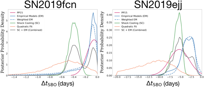
Figure 10. The posterior distributions of ΔtSBO for the four methods used in this paper, as well as a combined posterior based on the two most robust models (the shock-cooling and empirical models).
Download figure:
Standard image High-resolution imageTable 3. ΔtSBO and Resulting GSWs for SN 2019fcn and SN 2019ejj
| Method | SN 2019fcn | GSW (MJD) | SN 2019ejj | GSW (MJD) |
|---|---|---|---|---|
| Quadratic |

| [2458607.66, 2458609.90] |

| [2458587.43, 2458597.26] |
| Shock Cooling |

| [2458608.04, 2458609.91] |

| [2458595.01, 2458599.97] |
| Empirical Models |

| [2458608.42, 2458610.13] |

| [2458597.99, 2458605.68] |
| PP15 |

| [2458608.48, 2458610.12] | −5.30 ± 2.31 | [2458595.15, 2458601.37] |
| Combined (SC + EM) |

| [2458607.93, 2458610.16] |

| [2458596.39, 2458601.76] |
Note. The listed GSW MJD values correspond to 1σ ranges.
Download table as: ASCIITypeset image
We show the results of the simple quadratic polynomial fitting approach in Figure 2. As expected, the earlier detection of SN 2019fcn, with reasonable subsequent time sampling during the rise to the peak, leads to  days. For SN 2019ejj, the uncertainties are significantly larger, due to the later detection of the SN:
  days. As shown in Figure 10, the posterior distributions for ΔtSBO from the quadratic fit overlap the posteriors of the other methods, but tend to be broader, since the model is quite simplistic (due to the curvature staying constant; see the discussion of the bias in the appendix) and less physically informative.
The more physically motivated models provide tighter constraints on ΔtSBO. In Figures 3 and 4, we show the results of the shock-cooling model fits for SN 2019fcn and SN 2019ejj, respectively. We find that the model provides a good fit to the data, especially in the case of the rising portion of SN 2019fcn. We note that at later times (near the peak), there are some color mismatches between the data and the models, likely due to the more complex spectrum of the SNe compared to the model SED. We find that  days for SN 2019fcn and
  days for SN 2019ejj. The shock-cooling model also provides an estimate of the progenitor radius: (2.3 ± 0.3) × 103
R⊙ for SN 2019fcn and
days for SN 2019ejj. The shock-cooling model also provides an estimate of the progenitor radius: (2.3 ± 0.3) × 103
R⊙ for SN 2019fcn and  R⊙ for SN 2019ejj. The envelope masses are constrained to be
  M⊙ and
  M⊙ for SN 2019fcn and SN 2019ejj, respectively. Finally, we note that the model does not constrain the total ejecta mass (fpM); the posterior is approximately equal to the prior.
The data-driven approach, where we use empirical SN light curves as inputs, with some allowance for stretch, provide results that are comparable to the shock-cooling models, but tend to give systematically smaller values of ΔtSBO. Here we take the conservative approach of combining the posteriors of all nine input SNe, without down-weighting or discarding poorer fits.
8
Using the unweighted joint posterior from the nine input SNe, we find  days for SN 2019fcn and
  days for SN 2019ejj. In Figures 5 (SN 2019fcn) and 6 (SN 2019ejj), we show the posterior distributions for ΔtSBO and the stretch in phase for each of the nine input SNe. We find that for the less-well-sampled optical light curve (discovered at later times post-tSBO) of SN 2019ejj, there is some correlation between the stretch factor and ΔtSBO, such that a stretch larger than unity leads to a larger value and uncertainty associated with ΔtSBO. This is the case for the input SN light curves that are poorer matches to those of SNe 2019ejj and 2019fcn (and their respective light curves). For example, the fits from KSN 2011a, ASASSN-19jy, and ZTF19abqhobb would have benefited from an additional stretch (allowed in phase space), especially in regards to the fit of the second observed datum for SN 2019fcn, with the trade-off being a larger uncertainty assigned to tSBO.
Our final approach, using PP15, shown in Figure 9, provides good fits to the full light curves of both SNe, including, in particular, the rising phases of the light curves (see the insets in Figure 9). The resulting posterior distributions of ΔtSBO overlap with the shock-cooling and empirical models; in the case of SN 2019fcn, we find a better match to the empirical models, while in the case of SN 2019ejj there is overlap with both the shock-cooling and empirical model posteriors. Specifically, we find  days for SN 2019fcn and −5.30 ± 2.31 days for SN 2019ejj.
Finally, we construct a joint weighted posterior for ΔtSBO, using the posteriors of the shock-cooling and empirical models. We choose these particular models since they are more informative than the simplistic quadratic model and focus on the early part of the light curve (unlike PP15, which inherently leads to a compromise between matching the early and late parts of the light curve). At present, we do not strongly advocate for preferring the empirical model over the shock-cooling model, given their slight systematic offsets. However, in Appendix A.2, we perform a test to quantify the potential bias of the empirical model, which appears to be negligible. This seems to indicate that the shock-cooling model potentially tends to predict an earlier tSBO.
We use a combined posterior (using both the empirical and shock-cooling models), which gives an equal weight to both models. This combined posterior on ΔtSBO is shown in Figure 10 and listed in Table 3:  days for SN 2019fcn and
  days for SN 2019ejj.
To define the GSW, we shift ΔtSBO by a range of Δtcc = [1.4, 3] days, as we defined in Section 4.2. The final GSW durations computed using both the EOM from LVC20 and the methods presented in this paper are shown in Figure 11.
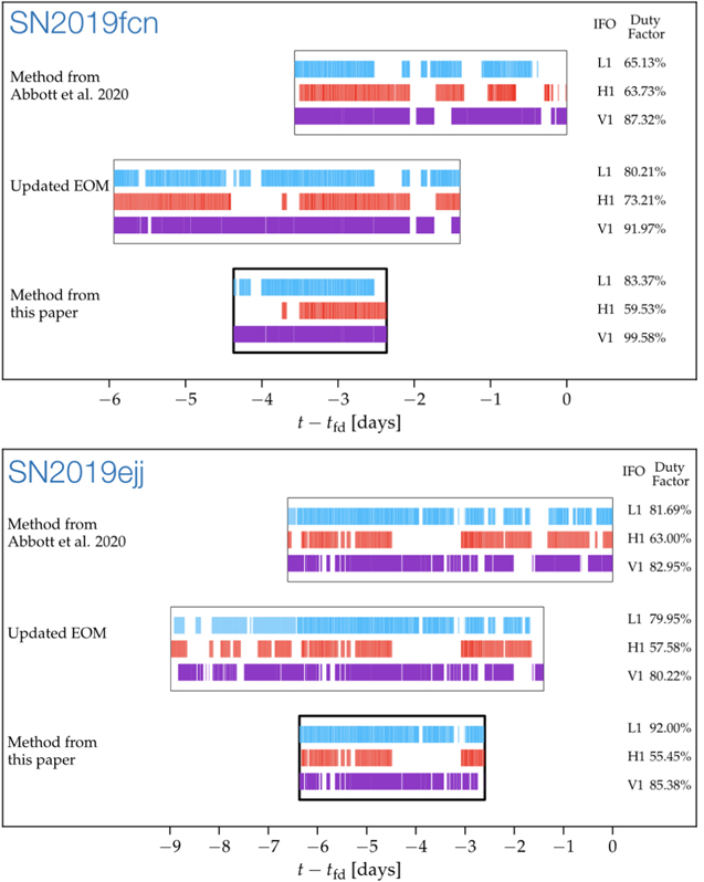
Figure 11. GSWs using the method presented in this work, compared to the EOM methodology of LVC20 and our update to that method. Our GSWs are narrower than those from the LVC20 method. Equally important, in the case of SN 2019fcn, we find a significant nonoverlapping region, suggesting that the LVC20 method may miss the time of GW emission. The horizontal colored regions within each GSW indicate the on-time of the three GW detectors (LIGO–Livingston, LIGO–Hanford, and Virgo), and the percentages on the right-hand side indicate the resulting duty factor. For both SNe, there is nearly 100% coverage with at least one GW detector during our calculated GSW.
Download figure:
Standard image High-resolution image6. Discussions
From the four methods presented in this work, the quadratic fit provides the most conservative (i.e., the widest-window) GSW, primarily because it is the least informative/a physics-based model. Especially in the case of delayed and poor sampling of the rising light curve, the posterior distribution of ΔtSBO from this model can be mostly noninformative (i.e., SN 2019ejj).
The physically motivated models provide much tighter constraints on ΔtSBO, but we note two possible trends based on the two SNe considered here. First, the shock-cooling model leads to an earlier estimate of tSBO compared to the empirical model approach; this difference is about 0.3 day for SN 2019fcn and about 2.4 days for SN 2019ejj (although there is more significant overlap in the posterior distribution in the case of SN 2019ejj). Second, we find that the PP15 model gives consistent results with the other two physical models; in the case of SN 2019fcn, it overlaps well with the posterior of the empirical models, while in the case of SN 2019ejj its bounds are in agreement with the posteriors of both the shock-cooling and empirical models.
We also note that both the shock-cooling and empirical model approaches can be improved. In the case of the shock-cooling model, better sampled early-time light curves will help to refine the model, resulting in more robust estimates of the various parameters, including the time of SBO. The shock-cooling model also has the advantage that it can provide a determination of the progenitor radius, which in turn may help to constrain the progenitor mass and the range of GW signals expected. We note, however, that this translation is not trivial, as the inferred radii may be affected by the presence of circumstellar matter (CSM) around the progenitor (Blinnikov 2017; Das & Ray 2017; Morozova et al. 2017, 2018; Singh et al. 2019; Nagao et al. 2020). 9
In the case of the empirical model approach, we anticipate a growing library of events from TESS that will help to better explore the parameter space of Type II SN early light curves. In this paper, we explore the effect on the estimation of tSBO from the scatter present in the library of light curves. We account for this additional correction by creating individual kernel density estimates (KDEs) for each light-curve model, which essentially act as a Gaussian PDF estimates. We then weight each model by the prior probability in both scatter and the stretch in phase. We then normalize the combined weighted KDE by dividing by the sum of the weights. This weighted combined posterior is shown in Figure 10. For the case of SN 2019fcn, the weighted posterior is in the same relative range as the empirical models, but with a smoothed single peak. For SN 2019ejj, the weighted posterior removes the bump at higher tSBO.
Finally, estimates of tSBO using the phenomenological models from PP15 could be further improved with detailed spectroscopic data during the rising phase of the light curve.
6.1. GW Detection Benefits
The statistical confidence of a GW candidate with a given false alarm rate (FAR) is quantified through the false alarm probability (FAP):

where ΔTGSW is the GSW duration. The reduction of the GSW by a factor of 2 allows a factor of 2 reduction in the FAP. In Figure 12, we show the impact of the GSW duration on the FAP as a function of FAR. We see that the method presented in the paper leads to a substantial improvement over the GSW durations from the LVC20 method. For example, for SN 2019fcn, a detection at FAR ≲ 1 yr−1 will have a significance of ∼3σ with our GSW.
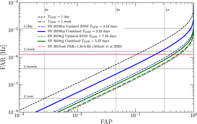
Figure 12. FAR as a function of FAP, along with the GSW durations for SN 2019fcn (blue) and SN 2019ejj (green). Also marked are fiducial GSW durations of 1 day (black dashed line) and 1 week (black dotted–dashed line). The vertical lines indicate the corresponding statistical significance of a detection at a given FAP. For SN 2019fcn, which has the narrowest GSW, we find that a detection with FAR ≲ 1 yr−1 will correspond to ∼3σ.
Download figure:
Standard image High-resolution image7. Conclusions
In this work, we have presented an astrophysically motivated approach for constraining the time of GW emission in targeted searches of CCSNe. The approaches presented here range in complexity from model-agnostic polynomial fits to model-dependent fits and a data-driven approach. We find general agreement between all approaches, with the most constraining results coming from the empirical model and the shock-cooling model. Using the combined posteriors of these models, we find an uncertainty on tSBO of ≈0.3 day for SN 2019fcn and ≈1.9 days for SN 2019ejj.
Thus, for SNe with well-sampled early light curves (such as SN 2019fcn), the resulting uncertainty on the time of SBO can be a few hours. In those cases, the dominant uncertainty on the final GSW (i.e., the time of core collapse and GW emission) is entirely influenced by current theoretical uncertainties in Δtcc—the time between core collapse and SBO. Here we take a conservative range of 1.4–3 days to encompass the model uncertainties and the unknown progenitor mass. Extracting information about the progenitor from the optical light curves and spectra may serve to reduce this uncertainty.
Our analysis continues to emphasize the importance of the early discovery and detailed follow-up of nearby CCSNe to further reduce the GSW for individual events that overlap LIGO-Virgo-KAGRA science runs. For the present, we stress that the GSW results provided here for SNe 2019ejj and 2019fcn should be used in searches of LIGO/Virgo Observing Run 3 for GW emission.
We thank Haakon Andresen, Sebastian Gomez, Evan O'Connor, Ondrej Pejcha, Tomas Prieto, David Sand, and Peter Williams for insightful discussions. The Berger Time-Domain Group at Harvard is supported by NSF and NASA grants. This research has made use of data, software, and/or web tools obtained from the Gravitational Wave Open Science Center, a service of LIGO Laboratory, the LIGO Scientific Collaboration, and the Virgo Collaboration. M.S. and M.Z. are grateful for computational resources provided by the LIGO Laboratory. M.S. is supported by National Science Foundation Grants PHY-0757058 and PHY-0823459. M.Z. is supported by NSF Grant PHY-1806885.
Appendix A: Assessing Methodology Reliability
One important item to assess is the reliability of each of the methodologies (described in Section 6) when estimating tSBO. We can assess this reliability by understanding the true error associated with each methodology. We define this as  , where MSE is the mean squared error, SV is the statistical variance, and B is the bias associated with each methodology. In this paper, we report the statistical variance (the uncertainty) associated with each posterior. It is important to note that all 1σ ranges reported in this work assume bias = 0.
A.1. Biases Present in the Quadratic Model
We removed 1–5 days' worth of data and used the remaining light curve to estimate tSBO for KSN 2011d, using the approach described in Section 4.1.1. We require that tSBO occur earlier than tfd, which we define as zero days. Table 4 lists the resulting tSBO estimates.
Table 4. Quadratic SBO Estimates for KSN2011d
| Days Removed from tfd | tSBO | χ2 |

|
|---|---|---|---|
| 1 | 1.26 ± 0.12 | 74 | 1.00 |
| 2 | 3.12 ± 0.34 | 113 | 1.52 |
| 3 | 3.01 ± 0.36 | 42 | 0.57 |
| 4 | 3.75 ± 0.35 | 38 | 0.51 |
| 5 | 4.16 ± 0.39 | 34 | 0.46 |
Note. We show that the later the light curve is discovered past SBO, the more the quadratic underestimates tSBO.
Download table as: ASCIITypeset image
The parameters of the polynomial model, tSBO, α, and β, give an approximation of the curvature associated with the early part of the light curve. We can define the rise time as − β/(2α). Having observations closer to the peak of the light curve forces the interpolation to be dominated by the curvature at the peak of the light curve, defined by α. If the magnitude of α is smaller than the average curvature of the light curve, 10 then the rise time will be overestimated. If the prior on α overfits the peak of the light curve, this also leads to an underestimation of tSBO.
A.2. The Efficacy of the Empirical Model
We discuss the efficacy of our empirical model fitting if there is not early photometry available for our nearby SNe. We estimate tSBO for two different scenarios: one with respect to a light curve that is complete (and therefore has access to tSBO), while the other one has only an incomplete, low-cadence light curve available.
We replicate the methodology described in Section 4.1.3 and use KSN 2011d as a test case for estimating tSBO. We removed 15 hr and 3 and 6 days' worth of data, and used the remaining light curve to estimate tSBO. We randomized which observational points were fed into the MCMC. We also rescale the associated error bars in order to understand the variance in the quality of both present and planned surveys (Chambers et al. 2016; Godoy-Rivera et al. 2017; Sand et al. 2018; Holoien et al. 2019; Vallely et al. 2021). High Cadence represents space-based surveys with Kepler-like cadence with error bars on the order of 10−4, whereas Low Cadence represents a ground-based survey cadence with error bars on the order of 10−2. This is shown in Figure 13.
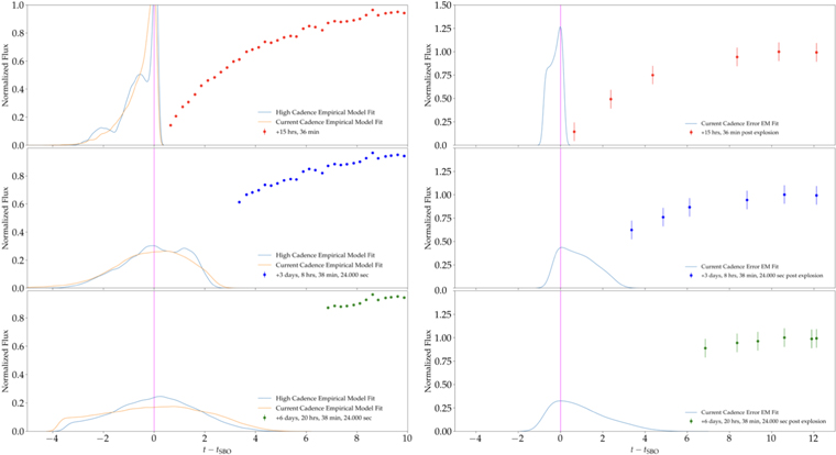
Figure 13. We show the resulting posteriors for our Kepler test. The left panel shows the resulting posterior for tSBO using all nine, with the original Kepler photometric points with both High and Current error bars. The right panel uses all nine light-curve models fitted to six randomized observed points from the light curve of KSN 2011d with Current cadence error bars.
Download figure:
Standard image High-resolution imageWe note a few things from Figure 13. First, both the High- and Low-cadence distributions are asymmetric. Second, the differences between the High- and Low-cadence resolutions were reflected their respective posterior shapes. Third, as expected, the posterior distribution became wider with decreasing rise information being fed into the MCMC. However, all posteriors were centered around the known value of tSBO.
Appendix B: Additional Models
B.1. Power Law
We fit the rising phase of an SNe following a dominating power law of the form

where tSBO is the time of first light (i.e., zero flux), and α and n are coefficients with no particular physical meaning. α is the flux on day 1, and n is the power-law index. We use an MCMC routine to fit for the three free parameters (α, n, and tSBO). For tSBO, we use a uniform prior set before first detection. For α and n, we use a uniform prior between two arbitrary bounds. We also fit for an intrinsic scatter parameter, σ, which we add in quadrature to the observational uncertainties, with a half-Gaussian prior peaking at 0 with a standard deviation of 0.1 in units of flux. Figure 14 shows the resulting fits.
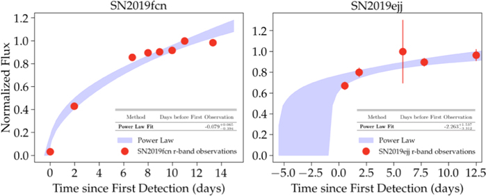
Figure 14. We show the power-law fits for both SN 2019fcn and SN 2019ejj.
Download figure:
Standard image High-resolution imageA well-sampled rise, as in the case of SN2019fcn, is fit relatively well, with minimal associated uncertainties, although tSBO is still underestimated. However, for the case for SN2019ejj, tSBO is underestimated by more than a few days.
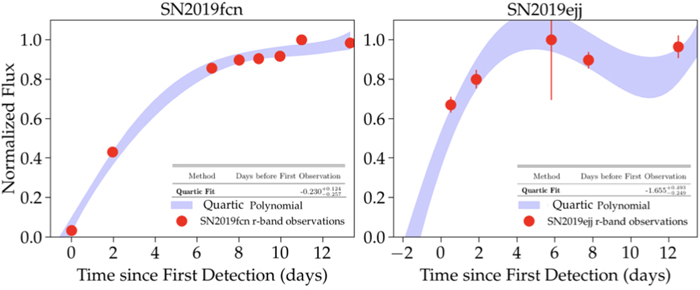
B.2. Quartic Polynomial
We also fit a fourth-order polynomial (quartic) to SN 2019fcn and SN 2019ejj. The same problems still persist with a higher-degree polynomial: the curve lands before the initial value of tSBO, because the data from [0, 2] days is narrower than the data for days [2, 12]. Therefore, the tSBO is underestimated. This is especially the case for SN 2019ejj, as shown in Figure 15.
Figure 15. We show the quartic fits from Appendix B for both SN 2019fcn and SN 2019ejj. The intersection of the blue region with the x-axis represents the 1σ range on tSBO for SN 2019fcn and SN 2019ejj. Since the rise was not well sampled in the case of SN 2019ejj, the quartic estimation of tSBO is underestimated and is much closer to the time of first observation.
Download figure:
Standard image High-resolution image
Footnotes
- 5
There were five additional CCSNe within ≈20–32 Mpc: SN2019hsw (Type II; Stanek 2019), SN2019ehk (Type Ib; Grzegorzek 2019), SN2019gaf (Type IIb; Swann et al. 2019), SN2020fqv (Type II; Forster et al. 2020), and SN2020oi (Type Ic; Forster et al. 2020). However, SN2019ehk and SN2020oi were Type I CCSNe, and for the rest we had insufficient early-time data, which disqualified them from the methods presented here.
- 6
Two additional fits using a power law and a fourth-order polynomial (quartic) are found in the Appendix.
- 7
For poorly sampled light curves (see the middle right panel in Figure 7), there is a correlation between ΔtSBO and the stretch in phase. Since we aim to use the Kepler and TESS light curves as empirical models of Type II SN light curves, we allow for a mild stretch, but constrain it using the log-normal prior.
- 8
We explore the effect on the estimation of ΔtSBO from the scatter present in the light-curve library by introducing a weighted combined posterior, discussed in Section 6.
- 9
If the presence of CSM biases the estimation of the inferred radii, this may lead to a potential biased offset in the estimation of tSBO. Although we explore the effect of any bias present in the empirical model in the appendix, the exploration of this effect in the shock-cooling model is beyond the scope of this paper.
- 10
β has no role in the curvature, since it has a linear dependence with time.