


Abstract
On 2013 June 21, a solar prominence eruption was observed, accompanied by an M2.9 class flare, a fast coronal mass ejection, and a type II radio burst. The concomitant emission of solar energetic particles (SEPs) produced a significant proton flux increase, in the energy range 4–100 MeV, measured by the Low and High Energy Telescopes on board the Solar TErrestrial RElations Observatory (STEREO)-B spacecraft. Only small enhancements, at lower energies, were observed at the STEREO-A and Geostationary Operational Environmental Satellite (GOES) spacecraft. This work investigates the relationship between the expanding front, coronal streamers, and the SEP fluxes observed at different locations. Extreme-ultraviolet data, acquired by the Atmospheric Imaging Assembly (AIA) instrument on board the Solar Dynamics Observatory (SDO), were used to study the expanding front and its interaction with streamer structures in the low corona. The 3D shape of the expanding front was reconstructed and extrapolated at different times by using SDO/AIA, STEREO/Sun Earth Connection Coronal and Heliospheric Investigation, and Solar and Heliospheric Observatory/Large Angle and Spectrometric Coronagraph observations with a spheroidal model. By adopting a potential field source surface approximation and estimating the magnetic connection of the Parker spiral, below and above 2.5 R⊙, we found that during the early expansion of the eruption, the front had a strong magnetic connection with STEREO-B (between the nose and flank of the eruption front) while having a weak connection with STEREO-A and GOES. The obtained results provide evidence, for the first time, that the interaction between an expanding front and streamer structures can be responsible for the acceleration of high-energy SEPs up to at least 100 MeV, as it favors particle trapping and hence increases the shock acceleration efficiency.
Export citation and abstract BibTeX RIS

Original content from this work may be used under the terms of the Creative Commons Attribution 4.0 licence. Any further distribution of this work must maintain attribution to the author(s) and the title of the work, journal citation and DOI.
1. Introduction
The acceleration of high-energy particles at the Sun is both an intriguing unsolved problem in plasma astrophysics and a key aspect of space weather science. The acceleration of so-called solar energetic particles (SEPs) from suprathermal energies up to relativistic energies is believed to occur during solar eruptions at flare sites, and at shock waves driven by coronal mass ejections (CMEs). The two-class paradigm, established about two decades ago, classifies the SEP events as either impulsive or gradual (Reames 1999; Desai & Giacalone 2016), according to SEP composition, time profile and spectra, charge states, longitude distribution of SEP associated flares, and acceleration source. It was proposed that impulsive SEP events are accelerated in solar flares, whereas gradual ones originate from the solar wind at CME-driven shocks. Nevertheless, this simplified empirical classification was soon challenged by the observation of hybrid events, i.e., gradual SEP events associated with impulsive soft X-ray events, or having elemental compositions and charge states at >10 MeV nucleon−1 that were similar to those found in impulsive SEP events at lower energies (Cohen et al. 1999, 2005; Richardson et al. 2000; Cane et al. 2003, 2007; Mewaldt et al. 2005, 2007; Papaioannou et al. 2016).
It has been shown that high-energy (above tens of megaelectronvolts) and low-energy particles may result from different seed and acceleration mechanisms dominating different energy regimes. In addition, it has been argued that different parts/stages of a solar eruption can act in concert to produce a variety of SEP signatures, and the re-acceleration of seed particle populations, coming from different coronal altitudes, may be important (Kocharov & Torsti 2002). For instance, interplanetary CMEs can re-accelerate seed particle populations coming from flares or seed particles produced by the CME liftoff/aftermath processes on a global coronal scale, apart from the eruption center. In order to account for the SEP properties of flares in large (gradual) events, three main scenarios were proposed, relating to: flare acceleration, the source of seed particles in the inner heliosphere, and shock geometry. Flare processes were proposed as the source of >25 MeV nucleon−1 ions (e.g., Cane et al. 2002, 2003, 2006, 2010; Klein & Posner 2005; Kocharov et al. 2005). Alternatively, the inner heliosphere could serve as a reservoir of suprathermal ions from a variety of sources; this includes material accelerated in flares, and suprathermal material accelerated at previous CME shocks (Mason et al. 1999; Desai et al. 2006). This material can be subsequently re-accelerated by CMEs that produce large SEP events. Finally, a variable shock geometry and compound seed populations were thought to be responsible for composition and charge state variability (e.g., Tylka et al. 2005; Tylka & Lee 2006). In this scenario, gradual SEP events are explained in terms of quasi-parallel shocks operating on seed populations dominated by solar wind suprathermals, whereas quasi-perpendicular shocks were thought more likely to accelerate flare suprathermals with higher-energy injection thresholds. The general consensus favors shock acceleration, over the alternative flare-based scenario, as the dominant mechanism in producing large SEP events (e.g., Reames 2013). However, significant gaps remain in our understanding of the detailed processes involved, and a combination of processes cannot be discounted.
Recent advances have been made by studying the evolution of CMEs and shocks in the lower and middle corona, the interaction with the underlying magnetic fields and coronal plasma, and the magnetic connectivity with in situ locations observing SEP events. Forward modeling techniques, based on multi-point imaging have been developed (e.g., Rouillard et al. 2016; Salas-Matamoros et al. 2016; Plotnikov et al. 2017; Kouloumvakos et al. 2019) to reconstruct the fronts of shock waves or CMEs by using different geometrical models, including spheroid (Kwon et al. 2014) or graduated cylindrical models (Thernisien et al. 2011). A study using a 3D model of coronal pressure waves was performed by Kouloumvakos et al. (2019) to derive shock parameters and compare them with properties of SEP events in 33 events with energies >50 MeV, which were clearly observed in at least two interplanetary locations by the Solar and Heliospheric Observatory (SOHO; Brueckner et al. 1995) and the Solar TErrestrial RElations Observatory (STEREO; Kaiser et al. 2008) spacecraft, during cycle 24. Significant correlations were obtained between the proton peak intensity during the prompt phase, and the shock speeds, compression ratios and Mach numbers for events with well-connected field lines, confirming previous results (e.g., Rouillard et al. 2016; Plotnikov et al. 2017; Afanasiev et al. 2018). However, no significant correlation was found with the shock angle, which is supposed to be an important parameter for the acceleration efficiency (Kozarev et al. 2015). In addition, a supercritical shock (fast-mode Mach number values in excess of three) seems to be needed at the release time of high-energy particles up to gigaelectronvolts (Rouillard et al. 2016). Nevertheless, further investigation is needed to understand the relationship between the observed features of SEP events and other important factors leading to their acceleration, such as the location of the acceleration region along the shock, and the role of the coronal magnetic field topology. Recent MHD simulations have shown the formation of shocks, or strong compression regions, at low coronal heights (<2 solar radii) at the flanks of an expanding CME, which can accelerate particles (Schwadron et al. 2015). It has also been suggested that the coronal/heliospheric neutral line could be a favorable region for particle acceleration, although spatially limited (Rouillard et al. 2016). The effect of large-scale streamer-like magnetic fields on particle acceleration at coronal shocks has been investigated through test particle simulations, when the streamer is aligned or rotated with respect to the CME propagation direction (Kong et al. 2017, 2019). In particular, the acceleration of particles to about 100 MeV can occur in the shock–streamer interaction region close to the shock flank possibly due to trapping effects. Alternatively, the gradual transition from oblique to quasi-perpendicular shock geometry during the CME propagation in the radial magnetic field has been shown to increase the acceleration efficiency (Sandroos & Vainio 2009). More recently, Wu et al. (2021) used a Monte Carlo simulation, which included bouncing and trapping effects, to investigate particle acceleration at shocks propagating along coronal loops. It was found that CME-driven shocks are also efficient accelerators of energetic electrons, generating hard X-ray emission, far from the flare.
In this paper, we provide observational evidence to support the premise that SEPs can be accelerated through an eruption-streamer interaction by studying the source region of an SEP event observed on 2013 June 21, the associated CME/shock expansion, and the interaction with streamers and pseudo-streamers (hereafter simply referred to as streamers). In Sections 2 and 3, we analyze extreme-ultraviolet (EUV), radio, and white-light (WL) observations of the event for the identification of the time-dependent CME/shock signatures and the resulting streamer deflection, as well as in situ SEP data to infer the particle release time. In Section 4, we use a 3D spheroidal model to reconstruct the expanding shock front as it passes through the corona, together with a potential field source surface (PFSS) extrapolation to estimate the magnetic connection with the SEP observing spacecraft. In Section 5, we derive the shock properties from radio and WL observations. Finally, in Section 6, we discuss the results and draw our conclusions.
2. Observations and Data Analysis
On 2013 June 21, an eruptive prominence, shown in Figure 1, was produced by active region 11777 (as classified by NOAA) located approximately at 14° S and 73° E, near the east solar limb, as seen from the Sun–Earth line. The eruption emerged around 02:35 UT, centered on angle 107° (measuring counterclockwise from solar north), and exhibited significant amounts of twist. The eruption produced associated coronal dimmings, observed predominantly to the south of the active region by the Atmospheric Imaging Assembly (AIA) on board the Solar Dynamics Observatory (SDO; Lemen et al. 2012). There is also some evidence of a faint coronal EUV wave associated with the eruption, emerging in all directions. The flare signature associated with the eruption was recorded as an M2.9 class flare, as observed by the Geostationary Operational Environmental Satellite (GOES-15). The flare growth phase began at approximately 02:32 UT, peaking around 03:14 UT.
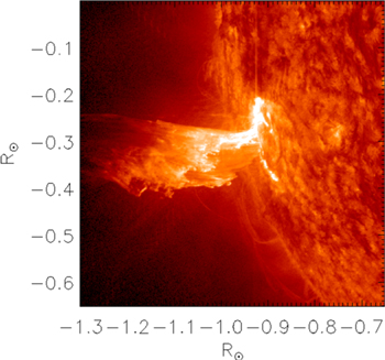
Figure 1. The prominence eruption as seen by SDO/AIA with the 304 Å filter (He) at 03:00 UT. The images have a field of view of approximately 0.65 × 0.65 R⊙.
Download figure:
Standard image High-resolution imageThe resulting fast, partial-halo, CME (≈1900 km s−1) rapidly passed through the AIA field of view (FOV), deflecting preexisting coronal streamer structures, and entered the Large Angle and Spectrometric Coronagraph (SOHO/LASCO; Brueckner et al. 1995) C2 FOV at 03:12 UT (Figure 2), and approximately 20 minutes later in the SOHO/LASCO C3 FOV.

Figure 2. An SDO/AIA 193 Å (03:11 UT) and SOHO/LASCO C2 coronagraph (03:12 UT) composite image, showing the expanding CME and deflected streamer structure to the north of the eruption (highlighted by the arrow).
Download figure:
Standard image High-resolution imageThe event was also observed by both the Sun Earth Connection Coronal and Heliospheric Investigation (SECCHI, Ahead and Behind; Kaiser et al. 2008) instrument suites on board the twin STEREO spacecraft, whose longitudinal separation from the Earth was −139 875 for STEREO-B and +139679 for STEREO-A on 2013 June 21. The fast erupting plasma was visible in the STEREO-B Extreme UltraViolet Imager (EUVI; Wuelser et al. 2004), 195 Å bandpass, from 02:35 to 02:55 UT and entered the COR1 WL coronagraph (Thompson et al. 2003) FOV at 03:00 UT. However, no lower coronal signatures were detected by STEREO-A at this time, because it was observed as a backsided event from the perspective of the spacecraft. Later on, at around 03:24 UT, the CME was seen to expand into both STEREO-A and STEREO-B COR2 coronagraph (Vourlidas et al. 2004) FOVs.
During the event, radio emissions were detected by both space- and ground-based instruments in different frequency ranges. In particular, the STEREO-B/SWAVES (Bougeret et al. 2008) and Wind/WAVE (Bougeret et al. 1995) spectrometers clearly detected type III and type II radio emissions in the decametric band, the latter implying the presence of a propagating interplanetary shock. SEPs were also detected by the Low Energy Telescope (LET; Mewaldt et al. 2008) and High Energy Telescope (HET; von Rosenvinge et al. 2008) instruments aboard both the STEREO spacecraft.
2.1. Extreme-ultraviolet Data Analysis
2.1.1. Temporal Intensity Variations
EUV data from SDO/AIA were used to study the temporal variations in the intensity observed during the formation, and early stages, of the eruption. The observations were combined with SOHO/LASCO WL imagery, and corresponding STEREO instruments, to study the expanding front in the plane of the sky (POS) and reconstruct the 3D shape of the shock front (see Section 4). The SDO/AIA (4096 × 4096 pixels) data were processed to level 1.5 using the IDL routine aia_prep.pro and normalized to their respective exposure times (by using the NORMALIZE keyword).
The top panels of Figure 3 show SDO/AIA observations of the prominence eruption and the expanding front at three different times through the 171 Å EUV passband (dominated by the Fe ix ion, with a peak temperature Tpeak ∼ 0.63 MK), whereas the bottom panels display corresponding running-difference (RD) images, constructed by subtracting the previously observed image.
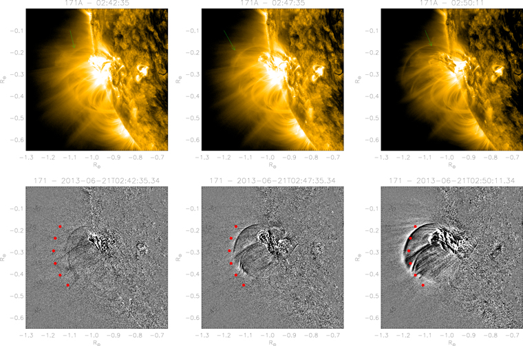
Figure 3. The expanding EUV front as seen through the SDO/AIA 171 Å passband (top panels) and the corresponding RD images (bottom panels) at three different times: 02:42, 02:47, and 02:50 UT, respectively, over a 0.65 × 0.65 R⊙ region. Red dots indicate regions where intensities were calculated, at different inclination angles with respect to the eruption foot-point. The green arrow highlights the expanding front.
Download figure:
Standard image High-resolution imageData from several SDO/AIA passbands were analyzed, the expanding bubble was also clearly visible through the 193 Å passband, which is dominated by two emission lines, from the Fe xii ion, which has a peak temperature of Tpeak ∼ 1.6 MK and the Fe xxiv ion at Tpeak ∼ 20 MK. As the bubble was observed to be fainter in the hotter 211 Å (Tpeak ∼ 2 MK) and 131 Å (corresponding to Fe xxiv with Tpeak ∼ 0.4 MK) passbands, it can be assumed that the Fe xii emission is dominating the 193 Å observations, which suggests that, in the region of interest, the emitting plasma was in the T ∼ [0.4–2] MK range.
Below 1.5 solar radii, the EUV spectral emission is believed to have a strong contribution from collisional excitation (Seaton et al. 2021), where the intensity Ii
is proportional to the plasma electron density ne
as  . Consequently, during the EUV front transit, if the only changing parameter is the electron density, the same temporal evolution would be expected to be observed in each SDO/AIA channel.
In order to study the possible temporal intensity variations due to temperature and/or density variations, we applied the following procedure (e.g., Ma et al. 2011; Chen et al. 2013; Vanninathan et al. 2015): we selected different directions with respect to the prominence foot-point, starting at a polar angle of 107° (counterclockwise from the north pole; indicated by the 0° line in Figure 3), and at two 15° positions to the north and three 15° positions to the south, to cover 75° in longitude and a large portion of the expanding front (see Figure 3, bottom panels). We defined angles to the north of the 0° line as positive, and those to the south as negative. A fixed position was selected along each of the angles, as indicated by the red dots in the lower panels of Figure 3, to compare the intensity at different times, and through different SDO/AIA passbands. Figure 3 shows the eruption at three successive times through the 171 Å passband. The same angles and positions were compared in the 131, 193, and 211 Å passbands.
As the erupting front was roughly semicircular in shape, and in order to make a meaningful comparison between the different angles, a fixed radial distance was selected at a distance of 350 pixels, corresponding to ∼0.22R⊙, along each line, as indicated by the red dots in Figure 3. At each position, an average intensity was calculated over a fixed circular region of interest (ROI) with an arbitrary radius of 10 pixels. The average intensity was calculated in each SDO/AIA data frame from 02:30 UT (flare onset) to 03:10 UT, after the erupting front left the SDO/AIA's FOV. The changing intensity with respect to time, in each of the AIA passbands, and at each angle is shown in Figure 4.

Figure 4. Shows the intensity as a function of time at each of the red points indicated in Figure 3 (bottom panels). The intensity is tracked in the 131, 171, 193, and 211 Å passbands. The horizontal dotted lines show the ±3σ level with respect to the average pre-EUV wave formation intensity (02:30–02:43 UT). Intensities values are normalized to unity for comparison.
Download figure:
Standard image High-resolution imageIn order to allow for a direct comparison between passbands, we normalized the intensities to unity. The following observations were made at the various position angles shown in Figure 4:
- 1.α = 30°: Observations from the 171 Å passband at the ROI first show a slow increase, above 3σ (background levels), around 02:45 UT. This is followed by an increase in the 193 Å passband approximately one minute later. Around 02:47 UT, the signals in the 131 and 211 Å passbands are also observed to increase. The increase cannot be attributed to the EUV/CME front at that time, as the front was still lower in the corona. However, faint and thin bright structures preceding the eruption are observed crossing the ROI, which can be associated with the pile up and deflection of the adjacent coronal streamer. The second peak in intensity was observed a few minutes later, indicating the arrival of the eruption, and was followed by a drop in intensity. The intensity of the 171 Å passband signal was at similar levels for both peaks. The differing times in the peaks in the different passbands suggest a more complicated thermal interaction, which is beyond the scope of this study. However, it is worth noting that the 171 Å passband signal is similar.
- 2.α = 15°: The initial intensity increase is observed at the ROI in the 171 Å passband around 02:47 UT, followed by a smaller second peak. One minute later, the 193 Å signal is seen to increase, followed by that observed in the 131 and 211 Å passbands, around 02:49 UT. At this angle, closer to the center of the eruption front, it is difficult to disentangle the signal from the perturbed surrounding streamer structure and the eruption front. The observed periodic oscillations in the 131 Å passband were probably due to a low signal-to-noise ratio.
- 3.α = 0°: The first peak is once again initially observed in the 171 Å passband, followed shortly after in the other channels, roughly between 02:48–02:54 UT. However, in contrast to α = 15° and 30°, the peak is broader (longer) and less well defined, and of lower intensity when compared to that of the second peak, as is indicative of a signal created by the pile up and displacement of material in front of the eruption front. The second peak is well defined, and created by the center of the eruption front, around 02:57 UT. The expanding CME front is followed by a broad noisy peak created by a part of the expelled prominence material.
- 4.α = −15°: The observed signal is similar to that seen in α = 0°, with a more pronounced third peak due to trailing prominence material.
- 5.α = −30°: At this angle, the eruption front is less well defined, and the signal is contaminated by co-temporal trailing prominence material. A small broad first peak is observed around 02:51 UT, probably created by material piled-up and displaced in front of the eruption, and followed by a multi-peaked signal from the eruption front itself, between 03:00-03:08 UT.
- 6.α = −45°: Exhibits a similar profile to that observed at α = −30°.
It is worth noting that the differing arrival times of the eruption front, observed between the different angles, can be attributed to the nonsymmetric nature of the expanding front. Also, in the lower corona, the eruption front and the shock front, if already formed, are difficult to disentangle due to their close proximity. When combined with line-of-sight (LOS) effects, due to the optically thin nature of the EUV observations, it is difficult to ascertain if the leading edge discussed above is created by the shock or the eruption itself. We also cannot discount the possibility that the shock front formed beyond the points of interest. In fact, the initial increases in brightness are more likely due to the CME leading edge crossing the points of interest, which supposedly is responsible for the streamer deflections, as will be discussed in the following section.
2.1.2. Interactions with Streamer Structures
The observations from low coronal heights show that the eruption emerged almost radially, but later expanded largely to the south. This may be due to the presence of streamer structures located to the north of the source region. Although it is difficult to ascertain the exact location of the foot-points of the streamers, their deflection due to the eruption can be evaluated, based on their distance from the source region. The top panel of Figure 5 shows successive images of the eruption from the AIA 171 Å passband, before, during, and after the eruption. The black line in each panel tracks a radial line from solar disk center at 117° (measuring counterclockwise from solar north), the white line tracks a line at 88°. The two lines encapsulate the region where the eruption is seen to emerge, as well as perturbed streamers located to the north of the eruption. The middle panel of Figure 5 shows a stack of 100 data slices taken from successive AIA 171 Å images at 30 second intervals. The data slices are taken along a line of constant radius at 0.18 R⊙, which is indicated by the gray arc in the successive top panels. The arc extends from 120° to 85° to capture the eruption and streamer movement to the north. The initial slice (at the bottom of the plot) is taken at 02:30 UT on 2013 June 21 and the last at 03:20 UT.
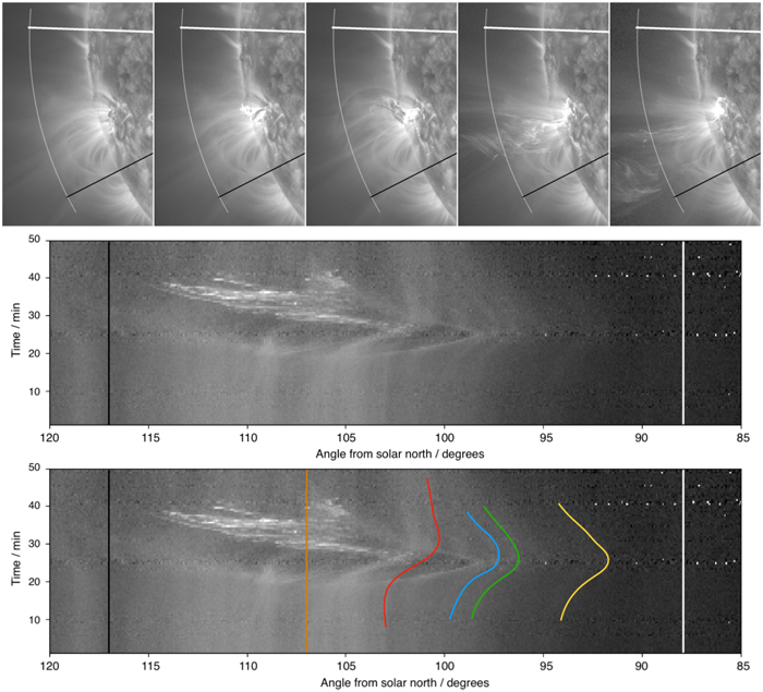
Figure 5. The top panels show successive images of the eruption on 2013 June 21 from the AIA 171 Å bandpass, at 02:30, 02:40, 02:50, 03:00, and 03:10 UT, respectively. The black line in each panel tracks a radial line from solar disk center at 117° (measuring counterclockwise from solar north), and the white line tracks an angle of 88°. The gray line is an arc of constant radius positioned at 0.18 R⊙ above the solar limb. The middle and bottom panels show a stack of data slices taken from successive AIA 171 Å images, along the line of constant radius at 0.18 R⊙ between 120° and 85° at 30 s intervals, with the first (bottom) slice taken at 02:30 UT on 2013 June 21 and the last (top) at 03:20 UT. The black and white lines mark angles of 117° and 88° from solar north, respectively. The orange line highlights the approximate direction of the center of the eruption, and the blue, green, yellow, and red points trace streamers 1, 2, 3, and 4, respectively, as discussed in this section.
Download figure:
Standard image High-resolution imageThe middle panel of Figure 5 highlights the dynamics of the eruption and its interaction with surrounding coronal features. Prior to the eruption intersecting the data slice along the gray arc (positioned at 0.18 R⊙), the slice is dominated by a series of white radial structures highlighting the positions of successive streamers, seen at the bottom of the panel. After approximately 20 minutes (at 02:50 UT), the eruption, centered on 107°, passes through the data slice. The twist in the eruption is evident from the oscillatory nature of the signature seen in the data slices between 20 and 50 minutes. There is also clear evidence of streamer deflection to the north of the eruption (right side of Figure 5, middle panel) through the bending of the surrounding white lines.
To estimate the degree of deflection of the surrounding coronal structures, four streamers/parts of a streamer were tracked by visual inspection of the data. The measurements were made in the plane of the sky and should therefore be taken as a conservative estimate of the deflection. The resulting deflections are more pronounced adjacent to the eruption; however, due to the optically thin nature of the EUV atmosphere, it is difficult to disentangle the eruption from the streamer signal, and therefore only streamers that did not observably overlap with the eruption are tracked, which also indicates that the measured deflections should be seen as conservative underestimates. Streamer 1 (blue line in the bottom panel of Figure 5), which was initially positioned at 997, is observed to deflect to 974 at its maximum extent, corresponding to a deflection of 16.7 × 10³ km. Streamer 2 (green) was displaced from 981 to 963, corresponding to a deflection of 13.2 × 10³ km, and, Streamer 3 (yellow) was displaced from 934 to 916, corresponding to a deflection of 12.9 × 10³ km. All three streamer deflections were measured by using an average of five separate measurements. After the eruption, the three measured streamers were observed to return back toward their initial positions; however, there is evidence that streamer 4 (red), which was not measured due to the optically thin argument above, does not return to its initial position, or at least, not in the time frame analyzed.
2.2. Radio Data Analysis
The solar event began with a very intense, long-duration, complex type III radio emission generated by beams of suprathermal electrons accelerated from the flaring region during the ascending and peak phase of the flare. These bursts often appear in radio dynamic spectra as bright and transient radio emissions that quickly drift from higher to lower frequencies with time.
According to the online Solar Geophysical Data (SGD), a first group of type III radio bursts, detected by the Culgoora Observatory, was emitted very low in the corona between 02:35 and 02:37 UT in the frequency range between 600 and 750 MHz. This episode nicely corresponds to the first peak observed in the flare light curve of GOES-15. Other groups of type III bursts were observed starting from 02:54 UT during the ascending phase of the second peak of the flare and are clearly discernible in the decametric range observed by one of the space-based radio spectrometers on board STEREO-B, as shown in Figure 6. This complex type III radio burst group was accompanied by a type IV radio burst observed with ground-based radio spectrographs, representing long-lasting broadband continuum emissions with variable time structure.
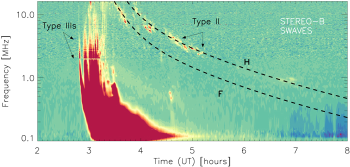
Figure 6. Radio dynamic spectra observed by STEREO-B/SWAVES (bottom) from 0.1 MHz to 16.025 MHz showing the type II and type III radio bursts associated with the CME between 02:00 and 08:00 UT. The black dashed curves are frequency–time profiles given by a double power-law model, obtained by fitting the frequency drift rate of the type II. The fitting gives two frequency–time curves corresponding to emission at the fundamental (F) and harmonic (H) of the plasma frequency.
Download figure:
Standard image High-resolution imageThe spectral properties and temporal evolution of the lower corona radio emission from 25 to 180 MHz provided by the ground-based Learmonth Solar Radio Spectrograph (LSRS; Western Australia), part of the USAF Radio Solar Telescope Network, are shown in Figure 7. The complex type III radio emission is also visible in the metric range, together with a possible fast-drifting type II lane at about 03:19 UT, not reported by the online SGD.
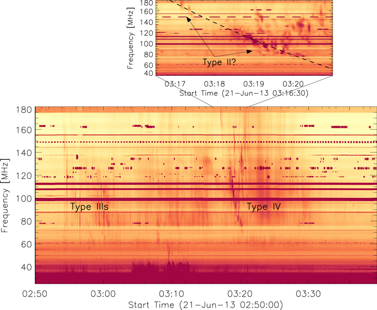
Figure 7. Learmonth dynamic radio spectrum in the 25–180 MHz frequency range, showing both type III and type IV radio bursts from 02:50 UT to 03:40 UT. A possible fast-drifting type II (harmonic) lane is also visible at about 03:19 UT.
Download figure:
Standard image High-resolution imageType II radio bursts are generated when electron beams, accelerated at the CME-driven shock fronts, interact with the ambient plasma. The produced radio emission has the local plasma frequency fpe and/or its harmonic frequency 2fpe, depending on the plasma density. Radio emission generated at progressively lower frequencies indicate that a CME-driven shock is propagating outward from the Sun, due to the decreasing density with helio-distance. In the decametric range, starting from about 03:30 UT, the fundamental and harmonic branches of a slowly frequency-drifting type II radio burst are also clearly visible in the radio dynamic spectrum of the STEREO-B/WAVES instrument as it propagated through the higher corona and interplanetary space (see Figure 6).
Observations from the STEREO-A/WAVES instrument did not show evidence of type II radio emission, while simultaneous observations from the Wind/WAVES space-based radio spectrometer showed a similar (but less intense) trace as evinced from the STEREO-B/WAVES radio dynamic spectrum.
2.3. The SEP Event
Early on 2013 June 21, the LET and the HET instruments on board the STEREO-B spacecraft recorded a noticeable increase in the energetic proton flux. Figure 8 shows the temporal profiles of the proton flux at energies from 4 to about 100 MeV in 17 differential energy channels. The observed proton flux increase had the typical behavior of well-connected SEP events: it was fast at all energies, followed by a slower decay, and extended to high energies. Specifically, the 60–100 MeV proton event began at 03:00 UT, reached a peak flux of about 3 × 10⁻³ cm−2 sr−1 s−1MeV−1 at 03:47 UT, and ended at 16:14 UT on June 22. Several minutes prior to the increase, a rise in the nonrelativistic electron flux was also recorded by the Solar Electron and Proton Telescope instrument (not shown here). The proton event at the lowest energies (4–4.5 MeV) started later at 03:45 UT, reached a maximum of about 70 cm−2 sr−1 s−1 MeV−1 at 19:50 UT, and declined to background levels over several days. A different shape was observed by the LET and HET instruments on board STEREO-A. Figure 9 displays the proton flux at energies from 4 to 23.8 MeV. It can be seen that the proton increase is weak, slow and significant only up to about 20 MeV, being consistent with an SEP event due to a late connection with a source (either the Sun, or a moving shock wave) originating from the eastern limb. Similarly, a small enhancement, up to about 10 MeV, was recorded at the Earth location, as observed in the GOES quick look plots; however, lack of available science data at the time of writing prevented a deeper investigation.
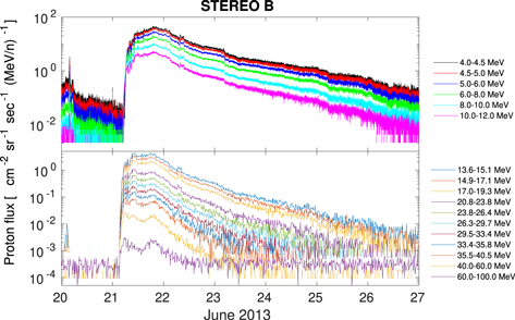
Figure 8. Temporal profiles of the proton flux at energies from 4 to about 100 MeV in 17 differential energy channels as detected by the LET (top) and HET (bottom) instruments aboard STEREO-B.
Download figure:
Standard image High-resolution image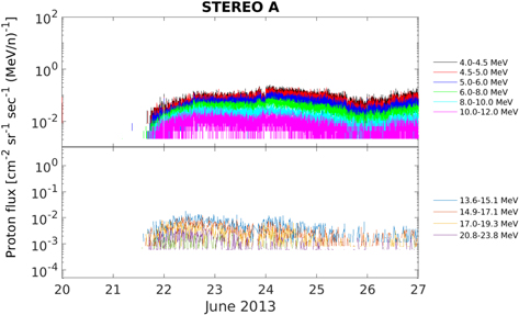
Figure 9. Temporal profiles of the proton flux at energies from 4 to 23.8 MeV as recorded by the LET (top) and HET (bottom) instruments aboard STEREO-A.
Download figure:
Standard image High-resolution imageIn order to evaluate the particles' release time at the Sun, we applied velocity dispersion analysis (VDA) to the known values of the observed onset times at 1 au and the particles' velocity (i.e., the square root of its energy normalized with respect to the proton rest energy; Laitinen et al. 2015). By assuming that the first particles observed at a given heliographic distance d from the Sun have been simultaneously released, that they propagate over the same path length, and that they experience no scattering, the arrival time ta to an observer at the distance s along the magnetic field line is simply given by

where to is the particles' release time at the Sun, s is the distance traveled, and v is the particle velocity. Thus, by knowing the observed onset times at 1 au and the speeds of the particles, we can evaluate the particles' release time at the Sun and the path length traveled by the particles. Figure 10 shows the onset time against particle inverse velocity, 1/β.
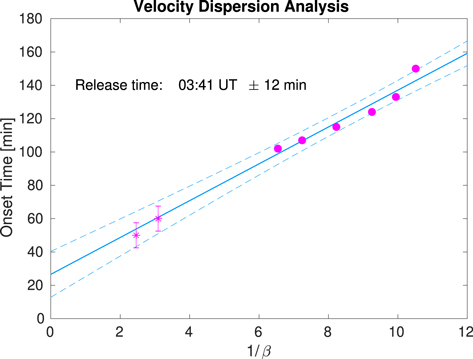
Figure 10. The behavior of the observed onset times and the inverse velocities, 1/β. Filled dots refer to STEREO-B/LET observations in the energy range 4–12 MeV, while asterisks refer to the highest-energy channels of STEREO-B/HET (i.e., 40–60 MeV and 60–100 MeV, respectively). The solid line depicts the best fit according to Equation (1), while the dashed lines are the 95% confidence levels. The release time, given on the top-left corner of the figure, is obtained as the intercept of the best-fit line with the y-axis and it is given in minutes after the solar flare.
Download figure:
Standard image High-resolution imageThe estimated release time of the particles at the Sun was at 03:41 ± 12 minutes UT, with a delay of about 1 hr from the flare onset time. We note that the VDA results need to be used and interpreted with care. Particles' scattering can produce poorly fitted results, since scatter tends to reduce the intensity, and thus statistically reduces the reliability of the observation. Moreover, the scattering mechanism can influence the particles' propagation. As a consequence, SEP events can vary widely in heliographic longitudes due to different types of particle transport mechanisms, which can in turn affect the velocity dispersion pattern. Thus, VDA can be seen as an estimate for time delays in the simplest way, which only considers scatter-free particles with no diffusion.
3. Shock Identification
3.1. Shock Identification from Radio Data
Unfortunately, no radioheliographic data are available for this event, so that the locations of the observed type II, III, and IV radio emissions are necessarily uncertain. In principle, notwithstanding the lack of such data, we can use measurements from radio receivers on board two or more spacecraft, at separate locations, together with radio direction-finding techniques to estimate the source location of solar radio bursts in 3D space (at long wavelengths; Makela et al. 2018). However, there was only a clear type II trace in STEREO-B/WAVES spectra, so the combined data from the two STEREO spacecraft could not be used for triangulation. Wind/WAVES data could not be used either, as the analyzed frequencies are not in the same range as those measured by STEREO, which would lead to the type II emission appearing to originate from a different source location (see discussion in Makela et al. 2018).
In order to relate the actual position of the type II emitting region (arguably located near the surface of the expanding shock) to the radio data, it is possible, in principle, to use the relationship between the plasma density and the heliocentric distance of the radio source region (see, e.g., Frassati et al. 2019) or, at least, to assume a heliospheric electron density model. The absence of radioheliograph observations for this event, however, implies that knowledge of the correct electron density distribution is not sufficient to give a reliable estimate of the type II source height. Notwithstanding the above caveats, we can still obtain a qualitative estimate by assuming radial propagation and a plausible density model.
A number of model density profiles have been derived both from radio and WL coronagraph observations. For a qualitative analysis of this event, we adopt the density model proposed by Mancuso & Avetta (2008) that used a formulation of the coronal electron density that is appropriate for solar maximum conditions. The fundamental branch of the type II radio burst was first visible in the STEREO-B/WAVES radio dynamic spectrum at 03:30 UT, corresponding to a frequency of ∼16 MHz and a distance of 3.2 R⊙. At 04:10 UT, according to the Mancuso & Avetta (2008) model, the radio emitting region was at about 7.3 R⊙. By using the density profile, the shock speed at 3:30 UT was about 1030 km s−1, while at 04:10 UT we find a speed of 1250 km s−1. Based on a linear fit to the data, obtained from the SOHO/LASCO CME Catalog (Gopalswamy et al. 2009), the CME speed was about 1900 km s−1 above 4 R⊙ at 03:12 UT, with an acceleration ∼1.46 m s−2. Accordingly, the electrons responsible for the observed type II emission must have been emitted at the flanks of the CME, which were expanding at a much lower rate. Similar results were obtained by adopting different electron density profiles taken from the literature. We also remark that a patchy type II lane was observed in the metric range by the LSRS at about 03:19 UT (see Figure 7). This radio emission was ignited at coronal heights between about 1.3 to 1.7 R⊙, as evinced by adopting the Newkirk (1961) density profile, that is, at a time when the front of the CME was near the border of the SOHO/LASCO C2 FOV (at ∼6 R⊙), again implying that the particles responsible for the type II emission were accelerated at the flanks of the shock. This is not unexpected, since the shock geometry in the inner corona is more likely to be quasi-perpendicular at the flanks, and efficient at electron acceleration, and subsequent type II burst excitation is mainly attributable to quasi-perpendicular shocks (e.g., Holman & Pesses 1983; Benz & Thejappa 1988), a feature that is present in our study case (see the following sections for a complete discussion).
3.2. Shock Identification from White-light Data
By inspecting the STEREO-B/COR1 (processed with secchi _prep.pro routine included in Solar Software) WL images, the CME features (cavity and leading edge) are clearly visible for the first time at 03:05 UT, as shown in Figure 11(a). The RD images reveal a faint feature at 03:10 UT that could be identified as a shock, which is indicated by the white arrows in Figure 11(b). This is not in contradiction to the findings from the EUV observations, because of the different FOVs in the POS. The shock was first identified in STEREO-B/COR2 (Figure 11(c)) and STEREO-A/COR2 (Figure 11(d)) images at 03:24 UT.
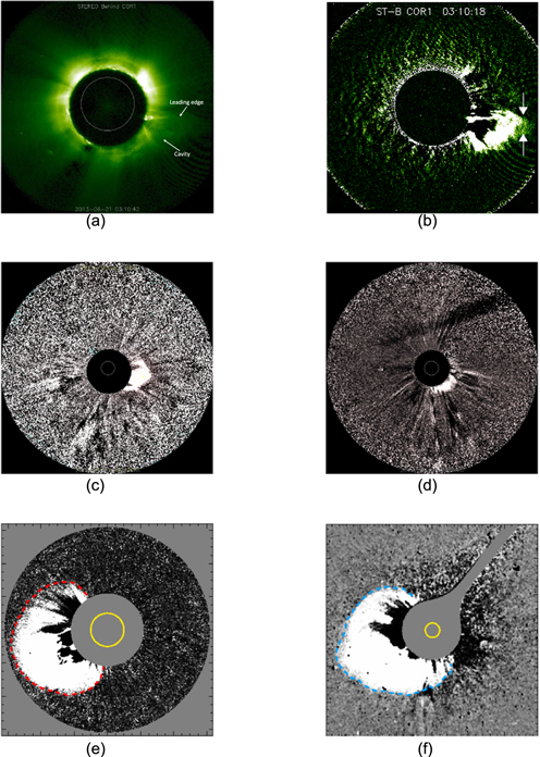
Figure 11. The CME and the shock RD images as seen by STEREO COR1, COR2, and SOHO/LASCO coronagraphs FOV at different times. (a) CME as seen by STEREO-B/COR1 at 03:05 UT. (b) The possible appearance of the CME-driven shock as seen in RD images of STEREO-B/COR1 at 03:10 UT. (c) The shock front as seen in STEREO-B/COR2 (RD image) FOV at 03:24 UT. (d) The shock front as seen in STEREO-A/COR2 (RD image) FOV at 03:24 UT. (e) The shock front as seen in SOHO/LASCO C2 (RD image) FOV at 03:24 UT. (f) The shock front as seen in SOHO/LASCO C3 (RD image) FOV at 04:10 UT.
Download figure:
Standard image High-resolution imageThe signature of the CME-driven shock front is first observed in WL images, from SOHO/LASCO C2, at 03:12 UT, at a height of ∼4 R⊙. It is observed as a faint emission enhancement, located ahead of the expanding CME, across the equatorial region. However, the whole shock front could only be identified in subsequent SOHO/LASCO C2 and C3 RD images, starting from the frame acquired by C2 at 03:24 UT. All images were processed using the SolarSoft IDL routine reduce _level _1.pro. To help better identify the faint shock front, the RD images were also appropriately filtered and contrasted in order to highlight the shock structure with respect to the ambient corona and the CME leading edge (see Figure 11 (e) and (f)).
4. 3D Reconstruction of the Expanding Front
In order to derive the most probable location of the SEP acceleration region, we reconstructed the 3D shape of the expanding front using EUV data from both SDO/AIA and STEREO/EUVI in the time range 02:45–02:55 UT, and coronagraphic images taken from STEREO/COR and SOHO/LASCO after 02:55 UT.
To help characterize the formation time of the shock, we used radio observations (Section 3.1), and an initial patchy type II lane radio burst was detected around 03:19 UT. However, a shock can be present also in the absence of a type II radio burst. A possible shock feature can also be seen at 03:10 UT (Figure 11), and so it is from this time that we consider the expanding front as a shock.
A spheroidal model, developed by Kwon et al. (2014) and implemented in the rtcloudwidget.pro routine included in the SolarSoft library, has been used by various authors (i.e., Mäkelä et al. 2015; Xie et al. 2017) to represent expanding fronts. The model is defined by three parameters:
- 1.the height h of the spheroid measured from the solar center, in units of solar radii;
- 2.the self-similarity constant κ = s/(h − 1), where s is the azimuthal semi-axis of the spheroid;
- 3.the eccentricity
 , for s > q where q = (h − 1)/2 is the radial axis.

In addition to these three parameters, we assume that the latitude and longitude of the source region of the event correspond to the location of the active region (S14 E73) as inferred from STEREO/EUVI observations just before the eruption. Subsequently, the settings were adjusted by visual inspection in order to match the wire-grid model, overplotted on each image, to the expanding front (where clearly visible) at approximately the same time in all coronagraph observations. As an example, Figure 12 shows the 3D grid reconstruction overlying the coronagraphic RD images at around 04:10 UT.
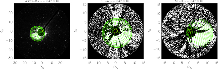
Figure 12. RD coronagraph images, from SOHO/LASCO C3 (left), STEREO-A COR-2 (middle), and STEREO-B COR-2 (right) at around 04:10 UT. The images are overlaid with green 3D grids representing the modeled shock front, obtained using a spheroidal model.
Download figure:
Standard image High-resolution imageIn order to study the temporal evolution of the expanding front, we fitted the s and q parameters obtained from the spheroidal model in locations where the moving feature was visible in observations from at least two instruments, through the time range 02:45–05:00 UT. We performed a second-order polynomial fit (Figure 13) for the first four data points, followed by a log-square fit (natural logarithm), which can be expressed as:
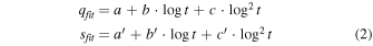
where a ( ), b (
 ), and c (
 ) are the q (s) fit parameters at time t.
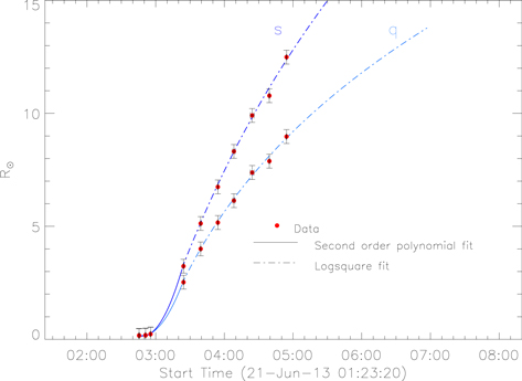
Figure 13. Shown here is a line of best fit to the spheroidal model azimuthal and radial semi-axis parameters, s and q, respectively. A second-order polynomial fit was used for the first four data points, and a log-square fit was used for the others. The error bars on the x-axis are derived from the time difference between measurements in the different instruments, meanwhile the uncertainties on the y-axis are a consequence of the visual inspection technique employed.
Download figure:
Standard image High-resolution imageThe uncertainties in the parameters are ±0.3 R⊙ for the ordinate axis, as a consequence of the visual inspection used to identify features in the STEREO/COR and SOHO/LASCO images (0.3 R⊙ corresponds to 5 pixels in STEREO-B/COR2 512×512 images). The uncertainties on the abscissa axis are derived from the difference in observation time between the different instruments. By using the relationships between the parameters characterizing the spheroidal model, we extrapolated the 3D shock evolution beyond the used coronagraph FOVs. The moving front evolved as a quasi-sphere during the initial phase of its expansion and then as an prolate ellipsoid when the front was above 2.5 R⊙.
4.1. Expanding Front and Magnetic Field
By using the 3D reconstruction of the expanding front, we calculated the angle, θBn, between the front and the coronal magnetic field. The magnetic field configuration was estimated using a PFSS (Schrijver & DeRosa 2003) extrapolation, from SDO Helioseismic and Magnetic Imager (HMI; Scherrer et al. 2012) measurements, made during the initial phases of the front expansion, between 02:45 UT and 03:10 UT, when the spherical surface was within 2.5 R⊙. This allowed us to estimate the compression/shock front geometry with respect to the background field reconstruction, and its role in SEP acceleration during the early evolution of the event. We note that the type II radio burst was clearly identified at later times, corresponding to greater heliocentric radial distances; however, possible shock formation signatures were identified from STEREO-B observations as early as 03:10 UT.
We thus assumed a potential field in the coronal volume, between the photosphere and a spherical source surface located at a height of 2.5R⊙, where the field was forced to become purely radial. The modeled magnetic field was based on the evolving full-Sun Carrington maps of the photospheric magnetic field. Since the boundary conditions are provided with a 6 hr cadence in the online PFSS database, we used the photospheric magnetic field closest in time to the event, corresponding to 2013 June 21 at 00:04 UT.
The PFSS extrapolation is shown in Figure 14 for the angle between the celestial north pole and the LOS from the Earth B0 = 0; the white lines correspond to the closed magnetic field, and the violet and green lines represent the open incoming (negative polarity) and outgoing (positive polarity) magnetic field, respectively.
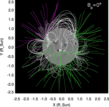
Figure 14. The extrapolated coronal magnetic field as obtained by the PFSS model from the photospheric magnetic field measured by SDO/HMI for B0 = 0, where the Earth is orthogonal to the figure. White lines correspond to closed magnetic field lines; violet and green lines represent open incoming (negative polarity) and outgoing (positive polarity) magnetic field lines, respectively.
Download figure:
Standard image High-resolution imageIn order to calculate the magnetic connectivity between the different spacecraft and the lower coronal shock front, we combined the 3D expanding front reconstruction, the PFSS extrapolation, and a model of the Parker spiral interplanetary magnetic field.
To this end, the shape of Parker spiral arms in the ecliptic plane connecting STEREO-A, STEREO-B, and Earth with the Sun was reconstructed by using the different solar wind speeds detected by the different spacecraft in the time range 02:24–14:24 UT, as reported in Table 1. We used the average, minimum, and maximum solar wind speed measured at each location during the SEP event. We also checked that no interplanetary CMEs were passing over the STEREO spacecraft during the SEP event, which may invalidate the Parker spiral assumption. On the contrary, at STEREO-B, the SEP event occurred on a high-speed stream.
Table 1. Solar Wind Speeds Measured by Different Spacecraft in Order to Reconstruct the Shape of the Parker Spiral Arms Connecting STEREO and Earth-based Spacecraft to the Sun
| Solar Wind Speed (km s−1) | |||
|---|---|---|---|
| Spacecraft | Average | Maximum | Minimum |
| OMNI | 472 | 447 | 508 |
| ACE | 471 | 438 | 508 |
| STEREO-A | 410 | 378 | 456 |
| STEREO-B | 531 | 493 | 594 |
Download table as: ASCIITypeset image
In the time interval 03:06–03:08 UT, only STEREO-B was found to be magnetically connected with the expanding front at the Sun, for which we were able to infer the inclination angle θBn. Such connectivity was found to be invariant with solar wind speed used (average, maximum, and minimum).
Figure 15 shows the geometry of the expanding front and the magnetic field just before, during, and after the connection between the front and STEREO-B. In this figure, the orange (green) portion of the expanding front represents the part above (below) the ecliptic plane; the blue, red, and green lines correspond to the magnetic field lines connected to STEREO-B, STEREO-A, and Earth, respectively. From Figure 15, it is evident that the magnetic line connected to STEREO-B (blue) was always quasi-parallel to the expanding front surface, so that it can be inferred that the front was quasi-perpendicular almost everywhere. We remark that the considered magnetic line is supposed to be representative of the global field configuration in the STEREO-B/front connection region, although its distribution is more complex (as is apparent in Figure 14).

Figure 15. The 3D geometry of the extrapolated expanding front, with respect to the magnetic field lines connecting the Sun to STEREO-B (blue), STEREO-A (red), and Earth (green), at times before (03:06 UT), during (03:07 UT), and after (03:08 UT) when the front was magnetically connected to STEREO-B. The yellow sphere represents the Sun, and the orange and green spheres represent the eruption front. The orange and green portions of the expanding front highlight regions above and below the ecliptic plane, respectively.
Download figure:
Standard image High-resolution imageIn order to explore the evolution of the shock geometry after 03:10 UT (>2.5 R⊙), we studied the intersection of the 3D expanding front, on the ecliptic plane, with the Parker spiral arms connecting to the different spacecraft.
From the right panel of Figure 16, it is evident that STEREO-B was magnetically connected to the shock front at an intermediate region located between the nose and flank. This connection is closer to the nose (flank) when using the maximum (minimum) solar wind speed to obtain the Parker spiral. This configuration can account for the intense and prompt increase in the STEREO-B proton flux (as shown in top panel of Figure 8). On the other hand, STEREO-A observed only a weak flux intensity (as shown in the bottom panel of Figure 9), which could be explained in terms of a late connection with the front. Indeed, it is apparent in Figure 16 that STEREO-A is only marginally connected with the shock front for all three solar wind speeds used to generate Parker spiral magnetic connections. Nevertheless, this could be an artifact of the assumed reconstruction model.
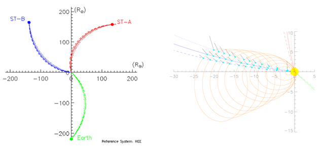
Figure 16. Shown here is the orientation of the Parker spiral arms as seen on the ecliptic plane. The left panel shows the orientation of the magnetic field lines connecting STEREO-B (blue), STEREO-A (red), and Earth (green) with the Sun, assuming average (solid lines), maximum (dotted lines), and minimum (dashed lines) solar wind speeds (see the text). The right panel shows a zoomed-in view of the Sun (yellow circle) and surrounding atmosphere, with the modeled emerging shock front at a 20 minute period from 03:24 UT (orange ellipses), with overlaid black lines representing the shock normal, at inclination angles θBn. The blue lines represent the magnetic connectivity to STEREO-B along the Parker spiral, assuming different solar wind speeds as in the left panel.
Download figure:
Standard image High-resolution imageIn order to know the shock geometry with respect to the magnetic field beyond 2.5 R⊙, we measured the angle θBn on the ecliptic plane between the normal to the shock surface and the Parker spiral. This was only done for STEREO-B, which has been found to be magnetically connected. The results show the expanding front to be quasi-perpendicular, for maximum solar wind speed (see Table 1), until 03:30 UT when the maximum helio-distance of the front, on the ecliptic plane, was around 5 R⊙. Beyond this height, the shock becomes quasi-parallel, having a minimum θBn ∼ 24° for the minimum solar wind speed of 493 km s−1. It is important to notice that the 3D extrapolation at later times (when the shock was no longer visible in any imagers) is affected by larger uncertainties because we have no information about the plasma properties, and so the θBn angles are no longer reliable.
5. Shock Properties from Radio and White-light Observations
In order to derive other important shock properties, we investigated the possibility of using observed patches of band-splitting episodes in the radio spectrum, to calculate the compression ratio, X. It is generally believed that the band-splitting is caused by the emission from the upstream and downstream shock regions (e.g., Smerd et al. 1974; Vršnak et al. 2001; Cho et al. 2007; Mancuso & Avetta 2008; Mancuso & Garzelli 2013; Chrysaphi et al. 2018; Kouloumvakos et al. 2021). In particular, Kouloumvakos et al. (2021) showed that type II bursts can be produced when a supercritical and quasi-perpendicular shock interacts with a coronal streamer.
As the observed frequency, f, is related to the electron density ne
by  , we can derive the compression ratio of the shock from the upper and lower frequencies in the band-splitting,
  , where nd
and nu
are the densities of the plasma downstream and upstream of the shock, respectively. fU
is the upper branch frequency, and fL
is the lower branch frequency of the band-split lane of the type II radio burst. In the interval between 04:10 UT and 04:12 UT, the only time when a clear band-splitting was observed, we find Xradio ≈ 1.3. In Figure 17, we show a detail of the radio dynamic spectrum observed by STEREO-B/WAVES (see Figure 6) that emphasizes the band-splitting episode used for the above estimate of the compression ratio.
, where nd
and nu
are the densities of the plasma downstream and upstream of the shock, respectively. fU
is the upper branch frequency, and fL
is the lower branch frequency of the band-split lane of the type II radio burst. In the interval between 04:10 UT and 04:12 UT, the only time when a clear band-splitting was observed, we find Xradio ≈ 1.3. In Figure 17, we show a detail of the radio dynamic spectrum observed by STEREO-B/WAVES (see Figure 6) that emphasizes the band-splitting episode used for the above estimate of the compression ratio.

Figure 17. Shown here are details of a clear band-splitting episode observed in the dynamic radio spectrum observed by STEREO-B/SWAVES (left panel), and a normalized intensity profile taken along the dashed blue line at 04:10 UT (right panel).
Download figure:
Standard image High-resolution imageIn order to infer the plasma compression ratio along the shock curves identified in WL coronagraphic data (see Section 3.2), we adopted the same method described in Bemporad & Mancuso (2010). The shock compression ratio was obtained by averaging the total brightness measured before (tBU ) and after (tBD ) the transit of the shock (i.e., in the first and second frames, respectively, which are used to compute the RD image in which the shock was identified) in small angular sectors located just "behind" the shock surface, and using the following relationship:

where F is the fraction of the pre-compression brightness originating only from the coronal region of finite thickness L along the LOS, subsequently crossed by the front. This factor can be estimated as
where the integration is performed along the LOS through the point located on the front, ϱ is the heliocentric distance of that point projected onto the plane of the sky (the "impact" distance), ne
(r) is the pre-compression coronal electron density, K(r, ϱ) is a geometrical function that takes into account the geometry of Thomson scattering and that is known exactly (see, e.g., van de Hulst 1950), and  . The value of the LOS integration length, L, was estimated from the observations using the same approach described by Bemporad & Mancuso (2010): the shock compression region is treated as a spherical shell with diameter D and constant projected thickness dproj. These parameters, which have been derived directly from the analysis of the WL images, were then used to estimate L across the shock, since, in this geometrical approximation,
  . The factor f defined in Equation (4) was inferred by using the electron density map derived from the SOHO/LASCO C2 polarized-brightness image acquired at 02:57 UT on the same day, i.e., immediately before the eruption of the CME.
Beyond the SOHO/LASCO C2 FOV, in order to calculate the plasma compression ratio from the SOHO/LASCO C3 measurements, we derived electron density profiles through a power-law extrapolation by assuming a radial dependence, proportional to r−2, and constrained by the in situ proton density value (∼10 protons cm−3) obtained with the WIND spacecraft (see Susino et al. 2015).
The resulting density compression ratio X profiles (shown in Figure 18) along the identified shock curves have a maximum around the shock nose, which is located at a polar angle, measured counterclockwise starting from the Sun's north pole, of about 120°−130° (30°−40° southeast in latitude) and decreases as a function of both altitude and time, suggesting a possible weakening of the shock, even though the harmonic emission of the type II radio burst was also observed at later times.

Figure 18. Density compression ratios, X, as measured along the shock front surfaces identified in SOHO/LASCO observations at four different times. The polar angle is measured counterclockwise starting from the north pole. Uncertainties in the measurements range from ∼5% for the values derived from C2 images up to ∼10% for the values obtained from C3 images.
Download figure:
Standard image High-resolution imageAccording to Susino et al. (2015), the major sources of uncertainty in the derivation of the plasma compression ratio are the uncertainty in the identification of the exact location of the shock in C2 and C3 RD images and the uncertainty in the electron density inferred from the inversion of LASCO polarized brightness. We estimated that the overall uncertainty affecting compression ratios is ∼5% for the values derived from C2 and up to ∼10% for the measurements obtained from C3.
Another important parameter of a shock is the Alfvénic Mach number, MA , which is useful to establish if the shock is supercritical or subcritical. In the solar corona, the plasma is dominated by magnetic phenomena due to the fact that
so, by assuming βplasma → 0 in the intermediate corona (see discussion by Gary 2001) and that the adiabatic index γ = 5/3, given the angle θBn measured between the shock normal and the upstream magnetic field, the relationship between the compression ratio X and the Mach number MA for different shock inclinations is given by (see Appendix discussion by Vršnak et al. 2002):
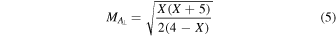
for a perpendicular shock ( ), and

for a parallel shock ( ). For the general case of an oblique shock, Bemporad & Mancuso (2011) estimated the Mach number
  by using the following expression:

The validity of the above approximate expression has been tested with the combined analysis of UV and WL observations of a shock wave (Bemporad et al. 2014) and numerical MHD simulations (Bacchini et al. 2015); the same expression has also recently been used by Kwon & Vourlidas (2018).
The angle θBn can be measured directly from coronagraphic images (at least for the projected fraction of the shock that is visible on the plane of the sky), by measuring the inclination angle between the visible shock front and the radial direction, and by simply assuming that the pre-eruption coronal magnetic field is radial above ∼2.5 R⊙. This hypothesis has recently been applied by Páez et al. (2019) to quantify the effects of corrugated shock fronts and their capability of accelerating particles. Given θBn and X along the front, measured in the POS, these values can be employed to measure both  and MA⊥, and also
  from Equation (7), thus obtaining the values that are plotted in Figure 19. As the X values are low, this leads to small values of the Mach numbers.
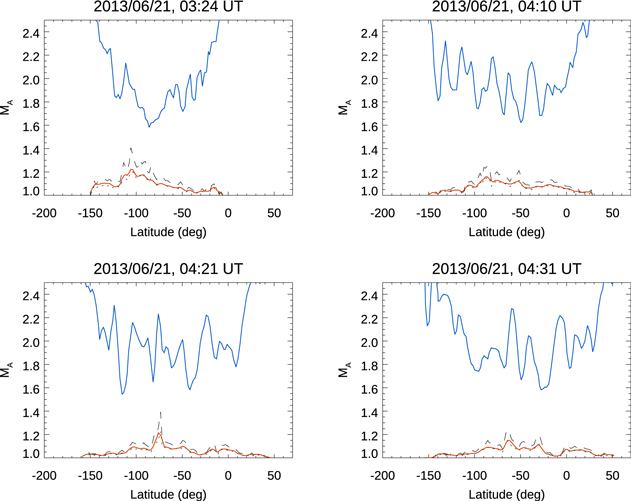
Figure 19. Plots of MA
along the four shock fronts, measured at angles counterclockwise from solar north, at four different times, identified in SOHO/LASCO WL coronagraph images (Section 3.2). Red lines represent  , while dashed (dotted) lines represent MA⊥ (
 ) values. For comparison, the blue lines identify
  values of critical Mach number. The top-left panel was obtained from SOHO/LASCO imagery on 2013 June 21 at 03:24 UT, the top-right panel at 04:10 UT, the bottom-left panel at 04:21 UT, and the bottom-right panel at 04:31 UT.
Download figure:
Standard image High-resolution image
As in Bemporad & Mancuso (2011), these curves can also be compared with the expected values of the critical Mach number  . Under the assumption that βplasma ≪ 1,
  mainly depends on θBn and varies between
  for perpendicular shocks and
  for parallel shocks (see Treumann 2009, Figure 2). Hence, the measurement of θBn also provides an estimate of
  along the shock front. The resulting values for this event (blue curves in Figure 19) show that the shock is subcritical at any time and at any latitude in the POS, at least in the time interval between 03:24 UT and 04:31 UT investigated with coronagraphic images. This result can also be confirmed by assuming that the critical value of the shock Mach number, needed for particle acceleration, as inferred theoretically by Vink & Yamazaki (2014), is equal to
  in the considered time interval. This result, however, does not exclude the possibility of the shock being supercritical in the early propagation phases, hence between 03:10 and 03:24 UT, when the type II radio burst emission was excited, or in the region where STEREO-B was magnetically connected (see Figure 16), but this methodology can not be applied.
6. Discussion and Conclusion
We analyzed the properties of the expanding CME-driven shock associated with the 2013 June 21 SEP event, produced by NOAA active region 11777. For this study, we used both space-borne and ground-based instruments: EUV imagers, WL coronagraph imagers, radio spectrometers, and particle detectors.
In Table 2, we summarize the times at which the flare, prominence eruption, CME, type II and type III radio bursts, and shock associated with the eruption were first detected in the different instruments.
Table 2. Times at Which the Flare, Prominence Eruption, CME, Type II and Type III Radio Bursts, and Shock Were First Detected in the Different Instruments
| Instrument | Spacecraft | First Detection | Event | Height (R⊙) |
|---|---|---|---|---|
| Time (UT) | ||||
| GOES | GOES-15 | 02:30 (Peak at 03:00) | Flare (M2.9) | |
| SDO | AIA-304 Å | 02:34 | prominence eruption | |
| Culgoora | 02:35 | type III radio burst | ||
| STEREO-B | COR1 | 03:05 | CME | 2.0 |
| STEREO-B | COR1 | 03:10 | CME and SHOCK | 2.7 |
| SOHO/LASCO | C2 | 03:12 | CME and SHOCK | ∼4.0 |
| LSRS | 03:19 | type II radio burst | ||
| STEREO-B | COR2 | 03:24 | SHOCK | 6.4 |
| SOHO/LASCO | C2 | 03:24 | SHOCK | 6.0 |
| STEREO-B | WAVES | 03:30 | type II radio burst | |
| SOHO | WIND | 03:35 | type II radio burst | |
| 03:41 | SEP release time | |||
Note. The measured height of the CME and shock nose are added for completeness.
Download table as: ASCIITypeset image
The event began with an M2.9 class flare, identified in GOES-15 X-ray light curves, and in radio frequencies (type III radio bursts at various radio observatories).
SDO/AIA EUV observations of the Sun, covering a global FOV of 2.54 R⊙, clearly showed an erupting prominence following the flare onset, in all passbands, especially in the 304 Å channel. Subsequently, a well-defined EUV wave was observed off-limb. The eruption and associated wave expanded largely radially, but with an evident southward deflection, as might be expected when an eruption emerges in the presence of a large magnetic structure such as a streamer, as seen to the north of the source region (Zuccarello et al. 2012).
By using the 131, 171, 193, and 211 Å channels, where this feature had greater contrast, we were able to perform a temporal analysis of the EUV intensity variations at different inclination angles (Figures 3 and 4) in order to understand its interaction with the surrounding plasma. In the time range 02:45–03:10 UT, when we were able to track the EUV wave, or at least part of it in AIA's FOV, the expanding front was interpreted as responsible for the streamer deflections observed in the lower corona. The movements of four deflected streamers were tracked (Figure 5): three of them returned roughly to their initial position in the time range 02:30–03:20 UT, but one (see the red line in Figure 5) did not, thus suggesting a prolonged interaction with the CME beyond 03:20 UT.
Visual inspection reveals a faint intensity increase leading the expanding front, at 03:10 UT, in the STEREO-B/COR1 coronagraph FOV. This intensity increase can possibly be associated with the CME-driven shock (Figure 11(b)), or at least to an area of compression. It is worth noting that the shock may have been present before the detection of a type II radio burst, but remained undetected.
At 03:12 UT, the expanding front entered in the SOHO/LASCO C2 coronagraph FOV. The density compression ratio was calculated from the WL observations between 03:24 to 04:10 UT, after the type II episode had already occurred and the entire shock front was clearly visible. Unfortunately, we were not able to use STEREO coronagraph observations for this analysis because COR1 is severely affected by stray light (see Figure 11(a)), while COR2 polarized-brightness images are partially affected by F-corona emission, making the measurement of compression ratios more uncertain (see Kwon & Vourlidas 2018).
By analyzing four images from SOHO/LASCO C2 and C3, we obtained density compression ratio XWL profiles, having a maximum around the shock nose and lower values at the flanks; the values decreased as a function of time-altitude (see Figure 18). The compression ratio reaches a peak, XWL = 1.5, around 120°–130° latitude at 03:24 UT, measuring counterclockwise from the north pole. The density compression ratio was also calculated using STEREO-B/SWAVES radio data at 04:10 UT, when the band-splitting was clearly identifiable (Figure 17), producing a value of Xradio ≈ 1.3. This value is in good agreement with the one found by the WL observations, in the region of the shock between the nose and the flank.
Due to the low values of the compression ratio, the calculated Mach numbers  and
and  are always lower than
  , allowing us to identify the shock as subcritical, at least in the time interval 03:24–04:31 UT.
Correspondingly, high-energy SEPs (up to at least about 100 MeV) were recorded at STEREO-B, which was found to be very connected to the EUV front/shock from 03:07 UT. However, the estimated particle release time occurred later at 03:41 ± 12 minutes UT, thus requiring an estimated acceleration time of at least ∼20 minutes.
Recently, shock regions of moderate to weak strengths have been found to be magnetically connected to locations (Parker Solar Probe; Fox et al. 2016; and STEREO-A) where the first widespread SEP event of solar cycle 25 was observed (Kollhoff et al. 2021). In particular, a subcritical shock was connected with the Earth (Kouloumvakos et al. 2021), where a particle increase was observed up to only 40 MeV. Nevertheless, the acceleration of high-energy particles in the solar corona usually requires strong and supercritical shocks (Kouloumvakos et al. 2019). The shock features obtained from the event studied in this paper do not seem to account for the recorded gradual SEP event and its energy content. This SEP event could be consistent with such a picture by assuming that the shock is supercritical between 03:10–03:24 UT, for which we do not provide an estimation. Alternatively, there is evidence of prolonged interaction between the compression/shock front and surrounding streamer structures through the observed deflection and recovery (in three out of four cases) of such structures surrounding the eruption in the lower and middle corona. Figure 5, shows a single slice through the lower corona at 0.18 R⊙ where deflections of at least 2 degrees are recorded. Although it is difficult to disentangle the position of the streamer from the eruption, due to the optically thin nature of the EUV observations, three streamers are observed to be displaced and recover over a period of more than 30 minutes between 02:30 UT and 03:20 UT, while a fourth does not recover over this time interval. By the latter time, the eruption will have emerged farther and be interacting with the streamers at greater heights. This interaction, along with the field orientation, seems to be conducive for particle acceleration. Simulations of a coronal shock propagating through a streamer-like magnetic field have shown that the acceleration of high-energy particles to 100 MeV mainly occurs in the shock–streamer interaction region, due to the perpendicular shock geometry and the trapping effect of closed magnetic fields (Kong et al. 2019).
When considering the coronal magnetic configuration and the Parker spiral in our observations, we found that the expanding front was quasi-perpendicular to the field orientation between 03:07 and 03:30 UT in the shock region (see Figure 16) between the nose and the flank, and connected with STEREO-B, supporting the above scenario. We suggest that a shock–streamer interaction might have also played a role in particle acceleration during the 2011 March 21 SEP event observed at STEREO-A and L1, where a good timing between streamer deflection and particle release was observed (Rouillard et al. 2012). The authors speculated that an initially quasi-perpendicular shock was likely developed near the base of the deflected streamers, on the CME far flank. However, they related the observed particle fluxes mainly to the speed and strength of the shock crossing the different connected magnetic field lines.
In addition, the interaction between the shock front and adjacent low-Alfvén speed streamer structures, due to the laterally expanding front, could also be an important source of both metric and interplanetary type II radio emissions, thus being responsible for the origin of the fast-drifting type II radio burst observed at 03:19 UT on 2013 June 21. Indeed, recent observations have shown that type II radio emission is often associated with the interaction between shocks and streamers (e.g., Cho et al. 2008; Feng et al. 2012; Chen et al. 2014; Mancuso et al. 2019; Kouloumvakos et al. 2021).
The small SEP enhancements (up to about 20 MeV) observed at STEREO-A can be explained in terms of a late connection to the extreme west flank of the shock (after 07:00 UT, under the assumption that the shock was expanding with a constant speed and crossing plasma with similar characteristics). As the STEREO-A magnetic foot-point was longitudinally distant from the flare location, by about 635, acceleration from the associated flare is an unlikely source, unless a very efficient cross-field transport is at work (Kollhoff et al. 2021). Nevertheless, it cannot be excluded, as recent SEP events have had their plasma sources confined to the foot-points of hot core loops of the associated flare (Brooks & Yardley 2021). This is compounded by the small angular separation between the flare location and STEREO-B foot-point (23°).
In conclusion, the CME/shock properties observed during the early expansion of the eruption, and the associated extended streamer structure deflections, provide evidence that the shock–streamer interaction can be a relevant factor for the acceleration of high-energy SEPs up to at least 100 MeV. Such an interaction creates conditions that are favorable for increasing acceleration efficiency; this includes particle trapping, and/or a perpendicular shock geometry.
The work performed here required the combined analysis of EUV, WL, and radio data sets, together with energetic particle flux measurements, acquired at three heliographic locations. Several recently launched missions to the inner heliosphere, including Solar Orbiter (Müller et al. 2013, 2020), BepiColombo (Milillo et al. 2020), and Parker Solar Probe, present unparalleled opportunities to advance this kind of study by exploiting more vantage points and high-resolution instrumentation. For instance, the observations being acquired by the Metis instrument (Antonucci et al. 2020; Fineschi et al. 2020; Romoli et al. 2021) on board the Solar Orbiter mission will potentially provide many more opportunities to study shocks associated with CMEs using these methods. Moreover, the multi-channel capabilities offered by this instrument will also provide a new view of these events, allowing us to measure not only the density compression, but also the temperature jump across the shock surface, thus providing a better understanding of these phenomena.
We are grateful to the SOHO, SDO, STEREO, Culgoora Observatory, and Learmonth Solar Radio Spectrograph teams for making their data available to us. The CME catalog is generated and maintained at the CDAW Data Center by NASA and The Catholic University of America in cooperation with the Naval Research Laboratory. F.F. is supported through the Metis program funded by the Italian Space Agency (ASI) under the contracts to the co-financing National Institute of Astrophysics (INAF): Accordo ASI-INAF n. 2018-30-HH.0. M.L. and A. B. acknowledge the Italian MIUR-PRIN grant 2017APKP7T on Circumterrestrial Environment: Impact of Sun–Earth Interaction.