


Abstract
Through phase-space mapping 6 yr of H+, O+, and  distributions measured in situ by the Mars Atmosphere and Volatiles EvolutioN (MAVEN) orbiter, we derive semiempirical average energetic neutral atom (ENA) distributions near Mars. Differential fluxes of H-ENAs and O-ENAs are estimated by line-integrating ENA production and loss rates in the average phase-space ion distributions. By repeating the procedure for a systematic series of vantage points, we produce synthetic ENA observations for virtual circular orbits with radii twice that of Mars, revealing the angular dependence of the observer's position. Accounting for known ENA production and loss terms, we find that H+ in the upstream solar wind yields total antisunward H-ENA fluxes of ∼3 × 105 cm−2 s−1. The dayside magnetosheath produces H-ENA angular-differential fluxes of up to 3 × 105 cm−2 s−1 sr−1, while the magnetosheath flanks populate the planet's nightside with H-ENA fluxes in the range of 104–105 cm−2 s−1 sr−1. The O-ENA environment is dominated by a near-isotropic ∼105 cm−2 s−1 sr−1 relatively low-energy (tens of eV) population originating in the top-side ionosphere, particularly on the dayside. Lower fluxes (103–104 cm−2 s−1 sr−1) of energetic O-ENAs (≳100 eV) are mainly found on the nightside and above the electric polar regions of the induced magnetosphere. Asymmetries in the ENA flow are largely limited to the energetic O-ENA populations, while the H-ENA distribution is mostly symmetric around the Sun‒Mars line. We discuss how synthetic ENA observations can provide insight into the near-Mars space environment, including the planet's plasma environment and exosphere.
Export citation and abstract BibTeX RIS

Original content from this work may be used under the terms of the Creative Commons Attribution 4.0 licence. Any further distribution of this work must maintain attribution to the author(s) and the title of the work, journal citation and DOI.
1. Introduction
Energetic neutral atoms (ENAs) are suprathermal atoms that can be created by the neutralization of energized ions in tenuous space environments. Upon neutralization, the ENA inherits the momentum of the progenitor ion and takes on a trajectory unaffected by the Lorentz force due to its neutral charge state. As such, observing ENAs effectively enables suitably equipped spacecraft to remotely characterize the plasma flow in planetary space environments (Futaana et al. 2006; McComas et al. 2011).
Ions can be neutralized by a few different processes. While electron recombination dominates neutralization rates in dense cold plasmas, charge exchange (CEX) between ions and neutral particles instead dominates at the suprathermal plasma energies and low densities that are typical of planetary exospheric space environments. Generally, the CEX ENA production rate depends on both the number flux of ions and the number density of neutrals, thus the resultant ENA flux carries convolved information about both the plasma and neutral distributions along the line of sight (LOS) of a suitable instrument (Futaana et al. 2011; Halekas et al. 2015). If one of these components can be constrained, then the other component could be deconvolved from the ENA measurements.
Mars lacks an Earthlike global magnetic field (Acuña et al. 1998), allowing the solar wind to penetrate deep into its exosphere, which is dominated by the hydrogen and atomic oxygen coronae (Chaufray et al. 2008; Clarke et al. 2014; Deighan et al. 2015). The solar wind is only deflected around 600–1000 km dayside altitudes (Trotignon et al. 2006) by the magnetic pressure generated by currents induced in the electrodynamic interaction between the solar wind and the planet's conductive ionosphere (Halekas et al. 2017; Ramstad et al. 2020). This induced magnetosphere deflects and shock-thermalizes the solar wind, thus forming a bow shock and a magnetosheath interfacing with the screened top-side dayside ionosphere. Because the solar wind penetrates deep into the Martian exosphere, the associated hydrogen-ENA (H-ENA) production rates are high, providing high fluences for ENA observations.
Relatively few ENA instruments have been flown on planetary missions. At Mars, the experimental designs of the Analyzer of Space Plasmas and Energetic Atoms (ASPERA–3) ENA detectors on the Mars Express orbiter (Barabash et al. 2006) provided the first empirical characterization of H-ENAs with energies over 100 eV. Measurements by the ASPERA–3 Neutral Particle Detector (NPD) indicated the presence of an H-ENA jet with fluxes of (4–7) × 105 cm−2 sr−1 s−1 emanating from the subsolar magnetosheath (Futaana et al. 2006), and slightly lower fluxes, 104–105 cm−2 sr−1 s−1, on the planet's nightside (Galli et al. 2008). The NPD measurements did not conclusively detect any oxygen ENAs (O-ENAs) from Mars above the instrument detection threshold, which implies an upper limit to the antisunward >100 eV O-ENA flux of 104 cm−2 s−1 sr−1 as measured in 2004 (Galli et al. 2006).
ENAs facilitate energy and momentum transfer for numerous processes at Mars, such as atmospheric sputtering (Shematovich & Kalinicheva 2020) and proton aurora (Deighan et al. 2018). Yet, the instrumental limitations and relatively short operational lifetimes (2004–2005) of the experimental ASPERA-3 NPD detectors have left the Martian ENA environment only superficially explored, and many open questions remain (Futaana et al. 2011). Low ENA energies and species other than H-ENAs are currently only accessible for investigation with models of the ionosphere‒solar wind interaction, which can be limited by assumptions and simplifications inherent to any model. With the resurgent interest in ENAs at Mars brought by the discovery of proton aurora, as well as the recent arrival of the Tianwen orbiter and its ENA-capable instrumentation (Kong et al. 2020), it is now timely to provide an empirical prediction of ENA distributions at Mars based on the comprehensive plasma measurements collected by the Mars Atmosphere and Volatile EvolutioN (MAVEN) orbiter (Jakosky et al. 2015) since its arrival at Mars in 2014 September. While MAVEN's suite of instruments does not enable the spacecraft to directly detect ENAs, the measured ion distributions combined with the context provided by the onboard magnetometer enable us to globally map ion flows near the planet and estimate ENA fluxes at any location in phase space.
2. Method
2.1. Neutral Densities
Determining ENA fluxes from CEX rates requires estimated ion and neutral distributions along a path where CEX occurs and ions flow, determined by some LOS. The density of the Martian exosphere is significant out to large distances from the planet, yet too low to be measured by the Neutral Gas and Ion Mass Spectrometer on MAVEN (Mahaffy et al. 2015). Instead, we use models for the cold and hot components of the H and O coronae, as well as thermospheric CO2 densities, by Valeille et al. (2010). Specifically, we adopt the one-dimensional parameterization by Modolo et al. (2016), shown in Figure 1(a).

Figure 1. (a) Neutral density profiles (1D) for estimating ENA net production rates near and upstream of Mars (Valeille et al. 2010; Modolo et al. 2016). The individual curves show the neutral CO2, O, and H densities as functions of altitude (left axis) and radial distance from the planet center (right axis). (b) Cross sections for CEX reactions with H+ (cold colors) and O+ (warm colors) as functions of energy (Lindsay & Stebbings 2005).
Download figure:
Standard image High-resolution image2.2. Phase-space Ion Distributions
The SupraThermal And Thermal Ion Composition (STATIC) instrument on MAVEN (McFadden et al. 2015) measures the local instantaneous ion flux distribution with 4 s cadence. STATIC's ion-optical assembly consists of an electrostatic deflector array, which sweeps the entrance elevation angle ± 45° for a top-hat electrostatic energy analyzer capable of selecting the ion energy per charge (E/q) between 0.1 eV/q–30 keV/q with an energy bandpass resolution ΔE/E = 16%, although the energy table used varies with time and location. A time-of-flight (TOF) system with a 15 kV preacceleration gap separates ions of differing mass per charge (m/q), with sufficient resolution to resolve major ion species such as H+, O+, and  . The ions are recorded by microchannel plate (MCP) detectors with 16 azimuthally sectored anodes, resolving the instrument's field of view (FOV) in 22
 5 bins. The full FOV is 360° × 90° for energies <5 keV, decreasing gradually to 360° × 15° at 30 keV. STATIC natively resolves each ion distribution in 16 azimuths, 16 elevations, 64 energies, and 1024 TOF bins, though binned to lower-resolution data products in order to reduce the required data downlink volume. Here, we use the STATIC d1 data product, in which each distribution is binned in 4 elevations, 16 azimuths, 32 energies, and 8 m/q bins, which can be unambiguously defined in the Mars‒Sun‒Orbit (MSO) reference frame. In Cartesian MSO coordinates, XMSO is defined by the direction to the Sun, ZMSO is parallel to the normal vector of the Martian heliocentric orbit, and YMSO completes the right-handed system.
To accurately determine the average ENA flux, the instantaneous (4 s) distributions need to be systematically organized according to the average global ion flow, which at high altitudes is mainly driven by the Lorentz force distribution in the induced magnetosphere. The orientation of the induced magnetosphere is controlled by the azimuthal clock angle of the upstream interplanetary magnetic field (IMF) (Riedler et al. 1989) and well represented by the corotating Mars‒Sun‒Electric field (MSE) reference frame (Dubinin et al. 1996). In Cartesian MSE coordinates XMSE is antiparallel to the solar wind velocity vector,
v
sw, ZMSE is defined by the direction of the solar wind motional electric field,
E
mot = −
v
sw ×
B
IMF, and YMSE completes the right-handed coordinate system. Here,
B
IMF is the IMF vector, which changes systematically and stochastically on a wide variety of timescales (Marquette et al. 2018), often shorter than the response time of the system. Lacking a dedicated solar wind monitor at Mars, we estimate the time-varying upstream IMF using measurements from the magnetometer investigation (MAG) on MAVEN (Connerney et al. 2015). Specifically, vector magnetic field measurements on orbit segments in the magnetosheath and undisturbed solar wind are low-pass filtered using a 30 min scale-length inverse exponential window function as described by Ramstad et al. (2020), providing interpolated estimates of the IMF vector in MSO coordinates also for orbit segments inside the induced magnetosphere and ionosphere. We estimate the IMF clock angle using the interpolated IMF vectors as  , though only include measurements for which the IMF is stable with a running standard deviation of
  , derived using the same window function used for ϕIMF.
In order to map the instantaneous ion distributions measured by STATIC in the MSE reference frame, we first correct the measured distributions for spacecraft potential and spacecraft velocity such that each measurement represents a sample of the local phase-space distribution in the Martian inertial frame. The ion distributions are subsequently transformed to the MSE reference frame by correcting for the average 4° solar wind aberration angle and rotating each measured distribution by −ϕIMF around the X-axis. We discretize the six-dimensional MSE phase-space domain by defining the average differential flux,  , as
, as

Here, S+ is the ion particle species (H+, O+, or  ), while the subscripts i, j, k, l, m, and n are indices that refer to elements in the discretized phase-space coordinate system. Xi
, Yj
, and Zk
represent MSE coordinates in the three Cartesian spatial dimensions, with each consecutive element separated from the next by a step size ΔX = ΔY = ΔZ = 0.1 RM. θl
, ϕm
, and En
are spherical coordinates in the energy-equivalent MSE velocity space, where each angular element is separated by Δθ = Δϕ = π/7 rad, and En
is logarithmically distributed from 0.01 eV to 30 keV in 33 steps. We go through all available MAVEN orbits from 2014 November to 2020 October and average element-wise all ion distributions measured by STATIC, excluding angular elements blocked by spacecraft surfaces and all measurements from sector 11, which is blocked by the harness for the instrument's attenuator (McFadden et al. 2015). The average differential flux is determined as
), while the subscripts i, j, k, l, m, and n are indices that refer to elements in the discretized phase-space coordinate system. Xi
, Yj
, and Zk
represent MSE coordinates in the three Cartesian spatial dimensions, with each consecutive element separated from the next by a step size ΔX = ΔY = ΔZ = 0.1 RM. θl
, ϕm
, and En
are spherical coordinates in the energy-equivalent MSE velocity space, where each angular element is separated by Δθ = Δϕ = π/7 rad, and En
is logarithmically distributed from 0.01 eV to 30 keV in 33 steps. We go through all available MAVEN orbits from 2014 November to 2020 October and average element-wise all ion distributions measured by STATIC, excluding angular elements blocked by spacecraft surfaces and all measurements from sector 11, which is blocked by the harness for the instrument's attenuator (McFadden et al. 2015). The average differential flux is determined as

where ι = 1, 2,..., NS,i,j,k,l,m,n are indices of the instantaneous differential flux measurements of ion species S+, made at times tι (which are disregarded), that sample the phase-space element [Xi , Yj , Zk , θl , ϕm , En ]. Phase-space elements of the H+ distribution upstream of MAVEN's orbit apoapsis are extrapolated by averaging all covered elements of the same velocity-space coordinates at XMSE > 2 RM. To demonstrate the resulting average ion distributions, we also integrate the average distributions over solid angle and energy in all spatial locations and display the resulting net H+ and O+ fluxes in Figure 2. The maps reproduce large-scale features expected to appear in the MSE reference frame. For example, Figures 2(d) and (h) clearly show the "plume" of O+ ions with energies of a few keV (Dubinin et al. 2006; Dong et al. 2015), scavenged from the ionosphere and picked up by the motional electric field of the solar wind flow, thus flowing largely in the +ZMSE ∣∣ E mot direction near the planet. Panels (a) and (b) show the deflection of the solar wind H+ bulk flow on the dayside with the divergence point offset in the + ZMSE direction due to mass loading of the solar wind near the planet (Dubinin et al. 2018). The deceleration and heating of solar wind H+ population are clearly apparent when comparing the velocity-space distributions between panels (e) and (f) as the distribution widens in the latter.

Figure 2. Time-averaged phase-space H+ (upper panels, blue colors) and O+ (lower panels, red colors) distributions mapped in the MSE reference frame based on MAVEN/STATIC measurements. Panels (a)–(d) show the spatial distributions of net H+ and O+ flux, integrated over velocity space. Panels (e)–(h) show average differential fluxes (circle size emphasizes high values) in velocity space corresponding to the four marked example locations in panels (a)–(d).
Download figure:
Standard image High-resolution image2.3. Estimating ENA Fluxes
ENA instruments measure the differential flux, j, of a neutral particle species, S, with energy, E, along an LOS. To produce comparable quantities, we estimate the relevant differential ENA production rates, P, and loss rates, L, integrated along the LOS (C) from an arbitrary vantage point, r, near the planet, yielding the total differential flux along the LOS as

Here, ds is an infinitesimal part of path C at spatial location  , whereas θ, ϕ, and E are spherical coordinates in energy-equivalent velocity space. At low energies, the planet's gravity has a significant effect on the particles' path in phase space from the point of production to the point of detection. We account for the effects of gravity and backtrace the particles' position in phase space along C, such that
  ,
,  , and E' are the velocity-space coordinates (
 ) of particles traversing along C at
  corresponding to particles that would be detected at [
r
, θ, ϕ, E].
corresponding to particles that would be detected at [
r
, θ, ϕ, E].
The CEX ENA production rate of species S can be calculated from the differential flux of its corresponding ion species S+, and the densities of secondary neutral species,  , as
, as

where Ss
can be any of the neutral species included here (CO2, O, or H) and the indices i, j, k, l, m, and n correspond to the phase-space element containing ![$[{\boldsymbol{r}}^{\prime} ,\theta ^{\prime} ,\phi ^{\prime} ,E^{\prime} ]$](https://content.cld.iop.org/journals/0004-637X/927/1/11/revision1/apjac4606ieqn13.gif) . The average differential flux
. The average differential flux  is empirically derived from MAVEN/STATIC measurements per Equation (2). The cross sections for CEX between S+ and Ss
,
is empirically derived from MAVEN/STATIC measurements per Equation (2). The cross sections for CEX between S+ and Ss
,  , are energy dependent and experimentally determined by Lindsay & Stebbings (2005), shown in Figure 1(b). Scattering effects are only included as kinetic-collisional loss rates, LS,col, with cross sections σcol, contributing to the total loss rate,

For the CEX neutralization rate, LS,CEX, we cannot approximate the ion species as stationary compared to the ENAs and have to solve the Boltzmann collision integral. The loss rate depends on the phase-space densities associated with the ENA flux and the ion distribution,


here defined in units of [cm−3 sr−1 eV−1]. The factors  and
and  are the speeds of the ENA and ion species, respectively. The relative ENA velocity with respect to each phase-space element is
  with corresponding energy
  . The CEX neutralization rate can be determined by integrating the differential rates over velocity space as
where  is the space angle of the phase-space angular element [θl
, ϕm
]. Lacking experimentally determined CEX cross sections for reactions neutralizing
is the space angle of the phase-space angular element [θl
, ϕm
]. Lacking experimentally determined CEX cross sections for reactions neutralizing  , we assume these are similar to the equivalent cross sections for O+. For the collisional loss term, LS,col, we only include collisions between the ENAs and other (secondary) neutrals, Ss
, as these are by far more numerous at nearly all altitudes. The collisional cross sections are determined by the kinetic radii, rS
, of each particle pair as
, we assume these are similar to the equivalent cross sections for O+. For the collisional loss term, LS,col, we only include collisions between the ENAs and other (secondary) neutrals, Ss
, as these are by far more numerous at nearly all altitudes. The collisional cross sections are determined by the kinetic radii, rS
, of each particle pair as  . The collisional loss rate can be determined by adding up the collision rates with all secondary species as

With production and loss rates determined along the LOS, the ENA distribution at any spatial location r can be determined by numerically evaluating the line integral in Equation (3) for a discretized domain of directions and energies. The step size (ds) cannot be infinitesimal in numerical integration. Instead, Equation (3) is iteratively evaluated forward along C as a Riemann sum using a finite step size (Δs) selected to be smaller than the typical length scales of the plasma and neutral distributions at any corresponding altitude, h. For computational efficiency, the values for Δs depend on altitude range as Δs(h < 300 km) = RM/ 100, Δs(300 km < h < 500 km) = RM/40, for Δs(500 km < h <6800 km) = RM/20 and for Δs(h > 6800 km) = RM/5. The loss rates at each step (Equations (8) and (5)) are calculated based on the differential ENA flux derived from the previous step with the initial value starting at zero, thus the derived ENA flux is unable to continuously grow in optically thick (i.e., collisional) regions.
Examples of ray-traced ENA fluxes are shown in Figure 3, here providing parts of the full distributions at the two shown convergence points. The rays correspond to the spatial location of C in Equation (3) and bend slightly near the planet due to gravity affecting the path in phase space. The nadir-looking rays require the smallest number of iterations (25 steps to 2 RM from the ray start at 100 km altitude), while more iterations are required for all other rays. The H-ENA rays are traced out to 30 RM upstream of the planet by extrapolating the upstream solar wind H+ distributions, and O-ENA rays are limited to the domain covered by MAVEN, i.e., within the ∼2.8 RM apoapsis of its original science orbit.
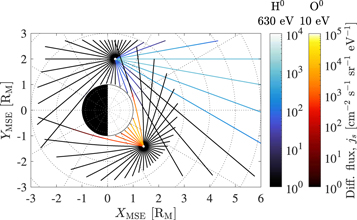
Figure 3. Ray-traced differential H-ENA (H0) and O-ENA (O0) fluxes in the MSE XY-plane as observed at two example vantage points (the convergence points).
Download figure:
Standard image High-resolution image3. Results
ENA distributions can in principle be estimated at any location relative to Mars using the described method, although only ENA sources and sinks within the domain covered by ion distributions can be included. In Figures 4 and 5, we explore the dependence of the ENA distribution on the observer's angular position around the planet. Each ENA distribution is calculated at systematically spaced vantage points along 2 RM circles in the MSE XY- and XZ-planes, analogous to circular orbits around Mars with a ∼3390 km altitude. All distributions are shown with an angular resolution of 10° × 10°, supersampled from a resolution of 5° × 5°. The four samples in each angular bin are averaged to emulate the angular coverage of a true particle detector.
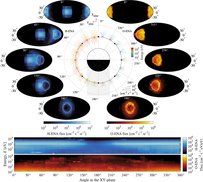
Figure 4. Average H-ENA and O-ENA distributions synthesized for a circular 2 RM orbit in the MSE XY-plane, i.e., the electric equatorial plane. Elliptical color panels show Mollweide-projected synthetic 10 eV–10 keV angular ENA distributions covering a 360° × ±90° FOV from a variety of vantage points on this orbit (marked by black dots). Arrows show characteristic energies associated with fluxes in this plane. Here, both angular distributions and arrows show H-ENAs on the left (0°–180°) and O-ENAs on the right (180°–360°) as the system is largely symmetrical across the ±YMSE hemispheres. Each angular distribution is centered on the +XMSE (− v sw or roughly sunward) direction and features a 30° × 30° grid. The Martian limb and terminator are projected as white contours for reference. The serial spectrograms show all synthesized H-ENA and O-ENA distributions integrated over the full 4π solid angle, i.e., the omnidirectional flux. The ENA distribution used to make this figure is provided as data behind the figure in the Common Data Format (CDF) (ENAdistXYorb.cdf).(The data used to create this figure are available.)
Download figure:
Standard image High-resolution image
Figure 5. Synthetic ENA distributions analogous to Figure 4, here in the MSE XZ-plane, i.e., the noon‒midnight plane oriented with E mot parallel to + ZMSE. Note that unlike in Figure 4, here the H-ENA and O-ENA angular distributions with panels at the same vertical position represent the same location around the planet. Additionally, all arrows indicate fluxes and energies of O-ENAs only. The ENA distribution used to make this figure is provided as data behind the figure in the Common Data Format (CDF) (ENAdistXZorb.cdf).(The data used to create this figure are available.)
Download figure:
Standard image High-resolution imageThere are several populations of ENAs that contribute to the distributions shown in Figures 4 and 5. Generally, there is a demarcation in the intensities and variabilities of both H-ENA and O-ENA distributions above and below ∼100 eV. Considering that fluxes <100 eV are also within one order of magnitude of the low-energy limit of this study and coincide with the detection limit of the ASPERA-3/NPD measurements, we henceforth take 100 eV as an otherwise arbitrary reference value when referring to low-energy and high-energy populations.
A relatively well-collimated beam of ∼800 eV H-ENAs with angular-differential flux up to ∼2 × 106 cm−2 s−1 sr−1 is persistent from the sunward direction throughout the near-Mars space environment, except near the planet's shadow. These are H-ENAs produced by neutralization of undisturbed solar wind upstream of the planet and thus form a narrow distribution. As such, the true distribution is not resolvable by STATIC, and a more meaningful number is the integrated flux of ∼3 × 105 cm−2 s−1 associated with this population (elements 10 eV–10 keV and within 45° from the Sun direction). The thermalized solar wind in the dayside magnetosheath also yields a wide distribution of high-energy H-ENAs with angular-differential fluxes up to 3 × 105 cm−2 s−1 sr−1 emanating from the dayside and flanks of the planet in all directions, visible from any vantage point with an unobstructed view of the dayside sheath.
Conversely, low-energy ENAs are dominated by populations originating in the ionosphere. In particular, the dayside and limb of the planet can be expected to figuratively glow in relatively high O-ENA fluxes of 105–106 cm−2 s−1 sr−1 dominated by energies ≲100 eV. At vantage points with angles ≳120° relative to the XMSE-axis (roughly the solar-zenithal angle), the dayside is largely hidden behind the limb. Instead, we find the view of the planet to be surrounded by a halo of O-ENAs with fluxes up to a few 105 cm−2 s−1 sr−1 at the limb and gradually decreasing with outward distance from the limb down to 103 cm−2 s−1 sr−1 and below outwards of ∼30° from the limb, as seen from the center of the tail. While H-ENA fluxes dominate over O-ENAs in most regions near Mars, inside the induced magnetotail, fluxes of the two species are comparable due to tailward O+ outflow (e.g., Lundin et al. 2008; Nilsson et al. 2012), as well as shadowing of the solar wind and dayside magnetosheath by the planet. Here, the strongest O-ENA fluxes can be seen originating from the ±ZMSE electric poles of the induced magnetosphere.
Otherwise, the induced magnetotail is largely invisible from vantage points outside the tail itself, whether observed either through H-ENAs or O-ENAs. This is largely due to the high directionality of >10 eV ions flowing downstream in the near-Mars induced magnetotail; therefore, the magnetotail ions only appear from vantage points on the nightside of the planet and near and inside the magnetotail. The pick-up-ion plume of scavenged ionospheric O+ ions (Dubinin et al. 2006; Dong et al. 2015) is also invisible from outside the plume for a similar reason. The O+ plume can clearly be seen in the maps of in situ measured ion distributions shown in Figure 2(d), specifically in the +ZMSE hemisphere above the planet, around the region marked by (h).
The full set of ENA distributions from which Figures 4 and 5 were created is provided as data behind the figures (ENAdistsXYorb.cdf and ENAdistsXZorb.cdf for Figures 4 and 5, respectively) and can be also be viewed and downloaded via the animations associated with Figures 6 and 7. The contents of each supporting data file are described in detail in Appendix C.
Figure 6. Supplementary animated version of Figure 4. Upper panels: angular H-ENA (cold color map) and O-ENA (warm color map) distributions (velocity space integrated over energies 101–104 eV). Lower panels: H-ENA and O-ENA omnidirectional energy distributions (velocity space integrated over solid angle). The concurrent angle in the XY-plane is indicated by a dotted line in the lower panels. The concurrent spatial location relative to the planet in MSE is also indicated by a white dot in the illustration on the right.
(An animation of this figure is available.)
Download figure:
Video Standard image High-resolution imageDownload figure:
Video Standard image High-resolution image4. Discussion
4.1. Sources of Bias and Error
The accuracies of the synthetic ENA distributions derived here are inherently limited by the accuracy of the ion distributions, neutral profiles, and cross sections used to derive them. For instance, the 225 × 225 angular resolution of the STATIC d1 data product is insufficient to accurately resolve the narrow solar wind distribution. In addition, ions scattering off STATIC's upper deflector support posts lead to a few percent of the true distribution appearing in other angular sectors and energies. Together with true variability in the solar wind direction and speed, these factors contribute to the apparent wide antisunward H-ENA distribution created from the neutralization of H+ in the upstream undisturbed solar wind. The instantaneous antisunward H-ENA distribution would appear much narrower in space angle and energy to an ENA instrument capable of resolving the distribution. The uncertainties in the CEX cross sections are comparatively small, below ±10% and ±15% for energies over and under 500 eV, respectively (Lindsay & Stebbings 2005).
Ignoring electron‒ion recombination as an ENA production term (e.g., O+ + e− → O0) could hypothetically imply that ENA fluxes emanating from the lowest altitudes are somewhat underestimated. Considering, however, that recombination cross sections are small and to first order depend on electron energy as  (Nahar 1999), recombination can only be a significant production term in the cold and dense lower ionosphere (∼130 km altitude), which is optically thick to ENAs. In the hot and relatively tenuous top-side ionosphere, from where the observable ionospheric ENAs are sourced, we take recombination rates to be negligible.
The largest source of systematic uncertainty is likely inherited from the coronal model by Valeille et al. (2010) and Modolo et al. (2016), mainly considering how unconstrained the exospheric structure was in 2010. In particular, the parameterized model is spherically symmetric, while in reality the exosphere has a three-dimensional structure (Chaffin et al. 2015) and also varies with season (Rahmati et al. 2018). In effect, ENA fluxes emanating from the near-planet nightside are likely overestimated due to the associated higher production rates, at least relative to the dayside.
Inaccuracies in the neutral densities at high altitudes would influence the total column density and thus the fluence of antisunward H-ENAs formed from undisturbed solar wind protons. Here, the estimated fluence of this population, ∼3 × 105 cm−2 s−1, increases to ∼7 × 105 cm−2 s−1 close to the planet, indicating that about 1% of the solar wind protons are converted to H-ENAs, an estimate consistent with those found by Kallio et al. (1997) and Halekas et al. (2017).
4.2. Comparisons and Caveats
Overall, the H-ENA fluxes on the order of up to 3 × 105 cm−2 s−1 sr−1 found here to emanate from the subsolar magnetosheath are largely consistent with Mars Express NPD observations (Futaana et al. 2006; Wang et al. 2019), particularly considering the unconstrained differences in upstream conditions and the instantaneous nature of the observations, as opposed to this time-average distribution. From a vantage point in the planet's shadow, the H-ENA fluxes from the magnetosheath flanks surrounding the planet are generally in the range of 104–105 cm−2 s−1 sr−1, which is also largely consistent with the MEX observations (Galli et al. 2008).
Synthetic ENA distributions are useful in a number of aspects. As described earlier, the ENAs carry information about both the plasma and neutral distributions along the LOS; however, actual ENA measurements are required to collect this information. Designing an investigation to measure ENAs strongly benefits from some understanding of the environment to be measured in order to optimize the orbit, operations, and instrumental properties, such as the energy range, sensitivity, and dynamic range. For example, we can clearly see in Figures 4 and 5 that the bulk of O-ENAs anywhere around the planet have energies <100 eV. Relatively weak fluxes of 0.1–1 keV O-ENAs appear at vantage points over the electric field pole (∼90° in Figure 5), likely originating as pick-up O+ undergoing the initial phase of acceleration. The most energetic (1–10 keV) O-ENA fluxes are only found at about 180°–240° in the MSE XZ-plane (Figure 5), originating near the planet in the −ZMSE hemisphere. For both of these energetic populations, the typical flux is 103–104 cm−2 s−1 sr−1; as such, it is perhaps not particularly surprising that the NPD on Mars Express with its lower-energy limit of 100 eV and 104 cm−2 s−1 sr−1 sensitivity threshold did not conclusively detect any O-ENAs (Galli et al. 2008).
With past or future measured ENA distributions in hand, comparisons with synthetic ENA distributions provide constraints on either the plasma or neutral environment. If the average ion phase-space distribution during actual measurements can be constrained, then exospheric models could be fitted such that the synthetic ENA distributions match the measured distributions. In this respect, we should consider that the ENA distributions derived here represent the estimated time-averaged near-Mars ENA environment, which is inherently dependent on the prevailing solar wind and ionospheric conditions, as well as the exosphere models used. While the average ion distribution (Figure 2) is produced using nearly all currently available and calibrated MAVEN STATIC data, this time period (2014 November–2020 October) was dominated by a deep solar minimum and any accurate comparisons with past or future ENA measurements may require constraints on specific upstream or seasonal conditions. ENA observations during other parts of the solar cycle will reflect the cycle's combined effect on the Martian plasma and neutral environments. Solar maxima are associated with increased solar extreme ultraviolet (EUV) ionizing radiation, which increases ionization rates in the upper atmosphere, in turn populating the hot oxygen corona through the dissociative recombination of  (Lillis et al. 2017). The increased ion production due to higher EUV levels also supplies more ions for outflow, though decreases the characteristic energy of the tailward outflowing ions (Ramstad et al. 2017). As such, we would expect low-energy O-ENA fluxes to increase drastically under high-EUV solar maximum and otherwise nominal solar wind conditions. The effect on high-energy O-ENAs is uncertain due to the competing effects of reduced solar wind–ionosphere coupling and increased CEX rates in the denser exosphere. Nevertheless, solar wind parameters are also far more variable during solar maxima and likely to yield at least periods of both stronger and higher-energy H-ENA and O-ENA fluxes as fast solar wind streams and interplanetary shocks interact with the planet.
These synthetic ENA distributions are also unable to reproduce dynamics and features that are not driven by the solar wind electric field, such as ENAs created by ion flows organized around the crustal fields (Wang et al. 2014) or other geographic features, which are smeared over time in the MSE reference frame. Additionally, there are other potentially significant ENA sources that do not produce ENAs through ion‒neutral CEX, such as backscattering (Kallio & Barabash 2000) and sputtering (Shematovich & Kalinicheva 2020), which would not be represented in these synthetic ENA distributions.
5. Conclusions
The solar wind motional electric field drives the orientation of the induced magnetosphere and organizes the O+ ion flows around the planet to a high degree (as shown in Figure 2), yet there is only a relatively modest corresponding effect on the bulk O-ENA distribution, mostly limited to the >100 eV range (the high-energy range as defined in Section 3). The typical O-ENA energy is overall strongly weighted toward the low-energy limit of this study at 10 eV. The low-energy O-ENAs are produced by suprathermal O+ ions in the top-side ionosphere (roughly altitudes 300–600 km), where exospheric densities and thus CEX rates are relatively high. Due to the relatively high O+ thermal velocities compared to bulk velocities, these low-energy O-ENAs can be observed in every direction, with particularly strong O-ENA fluxes emanating from the dense dayside ionosphere.
Higher-energy (≳100 eV) O-ENAs, on the other hand, can only be produced from O+ ions accelerated by large-scale or strong electric fields, such as the solar wind motional or Hall ( J × B ) electric fields. Not only do accelerated O+ populations feature relatively low fluxes under typical conditions, these also mainly occur at relatively high altitudes where the neutral densities are lower. In addition, CEX cross sections decrease with energy (see Figure 1). The net result is low fluxes of relatively high-energy O-ENAs, which mainly appear at vantage points on the nightside and at the ±ZMSE flanks. At the +ZMSE flank, the energy of the O-ENAs represents the early stages of ionospheric scavenging (Dubinin et al. 2006) and pick-up by solar wind in the magnetosheath. The energetic nightside O-ENAs are analogously produced from O+ ions accelerated largely toward the planet by the magnetosheath motional electric field, penetrating the magnetic barrier and passing through the denser regions of the exosphere. O-ENAs observed at the −ZMSE flank emanate from near the dayside limb and originate as O+ accelerated horizontally, possibly by Hall electric fields near the induced magnetic barrier.
From vantage points near the ±YMSE flanks (around 90°–130° and 230°–270° in Figure 4), O-ENAs incident from the dayside feature higher characteristic energies compared to those from the nightside. Ultimately, such differences in the O-ENA distributions reflect differences in the O+ flows toward the vantage points in both locations. We can infer that ions flowing near-horizontally from the dayside toward the flanks are energized up to 100s eV while ions circulating in the nightside near-planet ionosphere feature relatively low energies. The time-averaged nature of this analysis does not reveal the processes involved in producing these populations (though it does provide constraints); instead, future O-ENA measurements may reveal whether, e.g., time-varying instabilities at the solar wind interface (Ruhunusiri et al. 2016) or other processes produce the energetic O-ENAs and also map their extent.
Sources for H-ENA distributions are dominated by the solar wind and magnetosheath for the studied 10 eV–10 keV energy range. The hot dayside sheath emits H-ENAs in all directions, including sunward (from solar wind H+ that has completed at least one-half gyration in the sheath), with smaller contributions from ionospheric H+ at the lowest energies. Asymmetries in H-ENA distributions around the XMSE-axis are even smaller than for O-ENAs despite asymmetries in the H+ bulk flow seen in Figure 2. The lack of asymmetries in H-ENAs can be attributed to the hot H+ distributions in the magnetosheath and the employed spherically symmetric coronal models. Consequently, if analyses of measured magnetosheath H-ENAs reveal angular variations, then such variations are likely to reflect asymmetries in the structure of the true Martian exosphere.
There is a wealth of information about the Martian upper atmosphere, ionosphere, exosphere, and solar wind interaction that can be gained by comparing expected ENA distributions with actual measurements. The synthetic observations presented here are consistent with the available measurements from NPD on Mars Express, although more stringent comparisons with similar geometries and upstream conditions would be required to quantify any systematic differences. Considering the recently arrived Tianwen orbiter and also the potential for future ENA investigations at Mars, synthetic ENA observations provide timely and useful leverage for actual ENA measurements to advance our understanding of the near-Mars space environment.
This study was made possible thanks to NASA's Mars Exploration Program through its continued support of the MAVEN mission to Mars.
Appendix A: Animated ENA Distributions
While Figures 4 and 5 provide a summary of the predicted ENA distributions and the dependence of the observer's angular position around the planet, it is not feasible to show all of the 72 distributions derived for each virtual orbit plane in a pair of static figures. Instead, each angular distribution can be viewed animated frame by frame or downloaded via the animations associated with Figures 6 and 7. Omnidirectional spectrograms and the concurrent location of each frame in the respective orbit plane are shown for context. The animations effectively portray the predicted perspective of an omnidirectional 10 eV–10 keV ENA instrument circling Mars in a circular orbit at an altitude of 1 Mars radius over the surface.
Appendix B: ENA Statistics
The range of observable features in the system is limited by the ENA differential flux in relation to the sensitivity and dynamic range at any arbitrary energy of the hypothetical instrument in question. All figure panels above show ENA distributions integrated either over angular space or over energy (except the sparse ENA ray-traces in Figure 3). To provide a sense of the available domains of values, overviews of the range of fully differential fluxes in the system (from the vantage points along the investigated virtual orbits) are shown in Figures 8 and 9 in the form of two-dimensional histograms. We can see that the available domains of H-ENAs and O-ENAs are largely similar, although weighted differently with H-ENA fluxes stronger at high energies and O-ENA fluxes stronger at low energies. Indeed, the strongest derived differential fluxes are ∼10 eV O-ENAs reaching nearly 106 cm−2 s−1 sr−1 eV−1. Note that the virtual orbit in the MSE XZ-plane generally has more nonzero samples because the dense sampling near the velocity-space poles can be pointed toward the planet (near plane angles 90° and 270°).
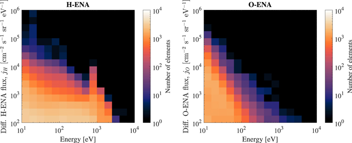
Figure 8. Histogram of all differential H-ENA and O-ENA fluxes derived from all ENA distributions in the virtual MSE XY-orbit.
Download figure:
Standard image High-resolution image
Figure 9. Histogram of all differential H-ENA and O-ENA fluxes derived from all ENA distributions in the virtual MSE XZ-orbit.
Download figure:
Standard image High-resolution image
Appendix C: Derived ENA Data Products
The ENA distributions derived here and used to make Figures 4–7 are provided in the Common Data Format (CDF) files ENAdistXYorb.cdf and ENAdistXZorb.cdf, which can be retrieved from the Figures 4 and 5 online or by request to the corresponding author. A description of the variables contained in the files is available in Table 1.
Table 1. List and Description of Variables in the Supplemental Files ENAdistXYorb.cdf and ENAdistXZorb.cdf that Are Available as Data behind Figures 4 and 5
| Variable Name | Size and Precision | Unit | Description |
|---|---|---|---|
| xmse | [1 × 72] single | km | Cartesian spatial MSE location (X) |
| ymse | [1 × 72] single | km | Cartesian spatial MSE location (Y) |
| zmse | [1 × 72] single | km | Cartesian spatial MSE location (Z) |
| th | [1 × 36] single | rad | Azimuth in MSE velocity space (θ) |
| ph | [1 × 18] single | rad | Elevation in MSE velocity space (ϕ) |
| E | [1 × 16] single | eV | Energy in MSE velocity space (E) |
| jHena | [36 × 18 × 16 × 72] single | cm−2 s−1 sr−1 eV−1 | H-ENA differential flux (jH) |
| jOena | [36 × 18 × 16 × 72] single | cm−2 s−1 sr−1 eV−1 | O-ENA differential flux (jO) |
Download table as: ASCIITypeset image