


Abstract
In this paper we present an extensive analysis of the GW190521 gravitational wave event with the current (fourth) generation of phenomenological waveform models for binary black hole coalescences. GW190521 stands out from other events since only a few wave cycles are observable. This leads to a number of challenges, one being that such short signals are prone to not resolving approximate waveform degeneracies, which may result in multimodal posterior distributions. The family of waveform models we use includes a new fast time-domain model (IMRPhenomTPHM), which allows us to extensively test different priors and robustness with respect to variations in the waveform model, including the content of spherical harmonic modes. We clarify some issues raised in a recent paper, Nitz & Capano, associated with possible support for a high-mass-ratio source, but confirm their finding of a multimodal posterior distribution, albeit with important differences in the statistical significance of the peaks. In particular, we find that the support for both masses being outside the pair instability supernova mass gap, and the support for an intermediate-mass-ratio binary are drastically reduced with respect to what Nitz & Capano found. We also provide updated probabilities for associating GW190521 to the potential electromagnetic counterpart from the Zwicky Transient Facility (ZTF) Graham et al.
Export citation and abstract BibTeX RIS

Original content from this work may be used under the terms of the Creative Commons Attribution 4.0 licence. Any further distribution of this work must maintain attribution to the author(s) and the title of the work, journal citation and DOI.
1. Introduction
GW190521 (Abbott et al. 2020b) is a uniquely stimulating gravitational wave (GW) event: it challenges our understanding of astrophysical formation channels of black holes, the accuracy of our waveform models, and our methods for data analysis (Abbott et al. 2020c; Nitz & Capano 2021; Mehta et al. 2021). The signal found is a very short transient with a duration of only approximately 0.1 s, and around four cycles in the frequency band 30–80 Hz (Abbott et al. 2020b). The source of the signal was originally identified as most likely being the merger of a binary black hole (BBH) system with a total mass of about 150 M⊙ in the source frame, the highest-mass merger observed to date. Furthermore, at least the more massive component was identified as having a very high probability of being inside the pair instability supernova (PISN) mass gap (Woosley 2017). In addition, a potential electromagnetic counterpart has been identified (Graham et al. 2020), although its association with the GW event is not considered robust (Graham et al. 2020; Ashton et al. 2020; Palmese et al. 2021; Nitz & Capano 2021).
For such short signals, it is however not surprising if GW waveforms corresponding to different source parameters fit the observed data equally well, and indeed already the original publication (Abbott et al. 2020c) by the LIGO Scientific and Virgo collaborations (LVC) discussed a wide range of possible alternative sources, and recent papers have proposed interpretations including that of a highly eccentric collision (Calderón Bustillo et al. 2021; Gayathri et al. 2020a; Romero-Shaw et al. 2020), a Boson star merger (Bustillo et al. 2021), a high-mass black hole–disk system (Shibata et al. 2021), or the first instance of an intermediate-mass-ratio inspiral (Nitz & Capano 2021). The latter paper found a trimodal posterior distribution, whose modes required a careful choice of priors and sampler settings to be resolved when running with the precessing frequency-domain model IMRPhenomXPHM (Pratten et al. 2021), which was developed recently, involving some of us.
For high-mass ratios, waveform models are not yet calibrated to numerical relativity (NR) simulations of precessing systems, and even the coverage offered by aligned-spin NR waveforms is sparse when compared to approximately equal masses. Therefore, modeling and extrapolation effects are expected to be significant and the impact of waveform systematics in this region of parameter space is still poorly understood. Indeed the possibility to choose among different precession prescriptions in IMRPhenomXPHM represents a useful tool to investigate the impact of different modeling approximations on parameter estimation. Frequency-domain waveform models such as IMRPhenomXPHM and its predecessors IMRPhenomPv2 (Hannam et al. 2014; Bohé et al. 2016) and IMRPhenomPv3HM (Khan et al. 2020) use a number of common approximations (see Ramos-Buades et al. 2020, for a recent discussion), in particular the "twisting-up" method, to represent precession effects starting from NR-calibrated aligned-spin waveforms (Hannam et al. 2014; Bohé et al. 2016), and the stationary phase approximation (SPA). Both strategies allow us to significantly accelerate waveform evaluation. The SPA is formally valid only in the slowly evolving inspiral phase, and its continuation into the highly dynamical merger-ringdown regime leads to inaccuracies that are likely to be particularly relevant for short-lived signals where only a few cycles around merger-ringdown are observed.
In order to gain a better understanding of the impact of different modeling approximations on parameter estimation results, we reanalyze GW190521 with different variants of IMRPhenomXPHM (García-Quirós et al. 2020b, 2020; Pratten et al. 2021) and the new phenomenological time-domain model IMRPhenomTPHM (Estellés et al. 2020b, 2020a, 2021c). Unlike its frequency-domain counterpart, IMRPhenomTPHM does not resort to the SPA approximation and offers a number of further improvements in the description of precession effects both in the inspiral and merger-ringdown regimes, including numerically evolved spin dynamics up to merger and an analytical approximation of precessing angles during ringdown. In this paper we will systematically compare results obtained with both models, following the strategy of a closely related paper (Mateu-Lucena et al. 2021) presenting a complete reanalysis of the GWTC-1 catalog (Abbott et al. 2019), as well as of another publication specializing on GW190412 (Abbott et al. 2020a; Colleoni et al. 2021), where similar systematic comparisons were carried out.
The purpose of this paper is twofold. First, we will clarify some of the challenges encountered in the analysis of high-mass non-vanilla GW events such as GW190521, in particular in terms of waveform systematics and robust Bayesian sampling. To this end, we will perform cross-comparisons between results obtained with two independent sampling codes, parallel Bilby (Ashton et al. 2019; Smith et al. 2020) and LALInference (Veitch et al. 2015). This is a particularly urgent task, as we expect the number of such atypical events to grow with the improvements in detector sensitivity. Second, we aim to provide improved parameter estimation results for GW190521 that might be useful to clarify its astrophysical properties. A key result is that we confirm the multimodal nature of the posterior found by Nitz & Capano (2021), but with some drastic quantitative changes due to improvements in the waveform models, in particular support for both masses being outside the PISN mass gap, and the support for an intermediate-mass-ratio binary are drastically reduced with respect to what was found by Nitz & Capano (2021).
The paper is organized as follows. We first discuss the waveform models we employ in Section 2, focusing on differences that are relevant for analyzing GW190521, and on how we can test robustness by comparing results from different models. We then summarize previous results from the literature in Section 3. In Section 4 we describe our methods for parameter estimation and for checking convergence and consistency between different prior assumptions. Readers interested primarily in new results may wish to skip to our results in Section 5, which is introduced by a subsection that briefly outlines the types of analyses we have performed and the results we have obtained. We give our final conclusions in Section 6 and discuss the dependency of the results on spherical harmonic mode content in the Appendix.
2. Waveforms
2.1. Notation and Conventions
We use the same notation and conventions as in our reanalysis of GWTC-1 (Mateu-Lucena et al. 2021). We will report all masses in units of the solar mass M⊙, and except where otherwise noted, we always refer to masses in the source frame, assuming a standard cosmology (Planck Collaboration et al. 2016; see Appendix B of Abbott et al. 2019). Some figures and tables use an "src" index as a more explicit notation for clarity. Individual component masses are denoted by mi
, and the total mass is M = m1 + m2. The chirp mass is  . We define mass ratios q = m2/m1 ≤ 1 and Q = m1/m2 ≥ 1.
We also define effective spin parameters, which are commonly used in waveform modeling and parameter estimation. The parameter χeff is defined as

where the χi are the projection of the spin vectors of the individual black holes onto the instantaneous direction perpendicular to the orbital plane. The effective spin-precession parameter χp (Schmidt et al. 2015) is designed to capture the dominant effect of precession, and corresponds to an approximate average over many precession cycles of the spin in the precessing orbital plane, and is defined in terms of the average spin magnitude Sp (Schmidt et al. 2015),


where A1 = 2 + 3/(2q), and χp is then defined as

Both χeff and χp are dimensionless and thus independent of the frame (source or detector).
We will employ waveforms with several multipoles beyond the quadrupolar contribution, always considering pairs of both positive and negative modes when referring to a particular multipole. Thereby, to refer to the example list of multipoles (l, m) = (2, ±2), (2, ±1), we will use the notation (l, ∣m∣) = (2, 2), (2, 1) or simply (2, 2), (2, 1).
2.2. Waveform Models Used
For a complete list of all of the waveform models used in the present paper, see Table 1. The original LVC publications on GW190512 (Abbott et al. 2020b, 2020c) used three families of waveform models, which represent incarnations of three well established approaches to compact binary coalescence (CBC) waveform modeling:
- 1.The SEOBNRv4PHM time-domain model (Ossokine et al. 2020; Babak et al. 2017; Pan et al. 2014): constructed within the effective-one-body (EOB) framework (Akcay et al. 2019; Bohé et al. 2017; Cotesta et al. 2020; Damour & Nagar 2016; Damour et al. 2015, 2013; Nagar et al. 2019, 2018; Nagar & Rettegno 2019; Nagar et al. 2017; Del Pozzo & Nagar 2017; Nagar et al. 2016; Pürrer 2016; Taracchini et al. 2012, 2014; Damour 2001; Cotesta et al. 2018).
- 2.The NRSur7dq4 surrogate time-domain model (Varma et al. 2019), which directly interpolates NR waveforms.
- 3.
Here we employ two further recently developed models that represent upgrades of IMRPhenomPv3HM and constitute a fourth generation of IMRPhenom models:
- 1.
- 2.IMRPhenomTPHM (Estellés et al. 2020b, 2021c), building on the non-precessing model IMRPhenomTHM (Estellés et al. 2020b, 2020c), which essentially applies the same phenomenological techniques at the heart of IMRPhenomXPHM to construct a native time-domain model. Working in the time domain allows several key improvements that we will discuss below.
Table 1. Waveform Models Used in This Paper
| Family | Full Name | Precession | Multipoles (ℓ, ∣m∣) | Ref. |
|---|---|---|---|---|
| SEOBNR | SEOBNRv4PHM | ✓ | (2, 2), (2, 1), (3, 3), (4, 4), (5, 5) | (Ossokine et al. 2020; Babak et al. 2017; Pan et al. 2014) |
| NR surrogate | NRSur7dq4 | ✓ | ℓ ≤ 4 | (Varma et al. 2019) |
| Phenom—Gen. 3 | IMRPhenomPv3HM | ✓ | (2, 2), (2, 1), (3, 3), (3, 2), (4, 4), (4, 3) | (Khan et al. 2020) |
| PhenomX | IMRPhenomXHM | × | (2, 2), (2, 1), (3, 3), (3, 2), (4, 4) | (García-Quirós et al. 2020, 2020b) |
| IMRPhenomXPHM | ✓ | (2, 2), (2, 1), (3, 3), (3, 2), (4, 4) | (Pratten et al. 2021) | |
| PhenomT | IMRPhenomTHM | × | (2, 2), (2, 1), (3, 3), (4, 4), (5, 5) | (Estellés et al. 2020b, 2020a) |
| IMRPhenomTPHM | ✓ | (2, 2), (2, 1), (3, 3), (4, 4), (5, 5) | (Estellés et al. 2020b, 2021a) |
Note. We indicate which multipoles are included for each model. For precessing models, the multipoles correspond to those in the co-precessing frame. For IMRPhenomTPHM, we also show comparison results with reduced sets of multipoles at several points in this paper, and in fact we use the ℓ ≤ 4 setting as a default run and comparison basis in most studies of alternative model options or priors.
Download table as: ASCIITypeset image
All of these models include a description of precession effects and subdominant harmonics, but do not include eccentricity, and they have complementary strengths and shortcomings that we will detail below.
Only NRSur7dq4 is calibrated to precessing NR waveforms, but its training data set is restricted to mass ratio Q ≤ 4 and dimensionless component spin magnitudes a1,2 ≤ 0.8). However the model can also be evaluated in the extrapolation region with Q ≤ 6 and a1,2 ≤ 1. Furthermore, usage of the model is restricted by the length of the original time-domain NR waveforms, and restrictions get tighter in the frequency domain due to the need of windowing before Fourier transforming the template. The limited length of NRSur7dq4 waveforms leads, in particular, to extra constraints on the minimum frequency and total mass allowed in parameter estimation analyses.
The IMRPhenom models describe precession via an approximate map between signals from non-precessing and precessing systems, which we will refer to as "twisting-up" (Schmidt et al. 2011, 2012; Hannam 2014). This approximation exploits the fact that, at least during the inspiral, the precession timescale is much slower than the orbital timescale, and thus the precessing motion mainly acts as an amplitude modulation. The spin of the remnant of the precessing system is however in general significantly different from the final spin of the non-precessing system. For a recent discussion of the approximations of this approach, see Ramos-Buades et al. (2020).
The SEOBNRv4PHM model (Buonanno et al. 2003; Babak et al. 2017; Pan et al. 2014; Cotesta et al. 2018; Ossokine et al. 2020) numerically integrates in the time domain the EOB BBH dynamics, including the spin-precession equations, using a Hamiltonian and GW flux that are tuned to non-precessing NR simulations. Then, the waveforms in the inertial frame are obtained by applying a time-domain rotation ("twisting-up") to the waveforms in the co-precessing frame (Buonanno et al. 2003; Babak et al. 2017; Pan et al. 2014).
Neither the SEOBNRv4PHM nor IMRPhenom models include the asymmetries between positive and negative m spherical harmonic modes in the co-precessing frame, which are related to the large recoil velocities observed in some NR simulations of precessing binaries, as discussed in Bruegmann et al. (2008).
We now turn to describe relevant aspects of the IMRPhenomX and IMRPhenomT families, which we use for the new results presented in this paper. Frequency-domain waveform models are particularly attractive for GW data analysis, since they are naturally adapted to a matched-filter-type analysis, where the noise is characterized in the frequency domain, and accordingly allows the most computationally efficient Bayesian inference analysis. In order to accelerate the evaluation of precessing waveforms, current frequency-domain IMRPhenom models also use the SPA approximation to compute the transfer functions between the frequency-domain non-precessing waveform and the precessing waveform in an inertial frame (see Marsat & Baker 2018 for more accurate alternatives). The assumptions underlying the SPA fail for merger and ringdown, but the method has been found to work surprisingly well, and has been routinely used in GW data analysis; see, e.g., Abbott et al. (2019) and Abbott et al. (2021a). The approximation does however have to be employed with caution when essentially the only observable part of the signal is the merger and ringdown, as is the case for GW190521. This shortcoming has been one of the main reasons for us to also develop a time-domain phenomenological waveform model, IMRPhenomTPHM, which does not rely on the SPA. One of the goals of this paper is to discuss in detail how to avoid misleading conclusions from analyzing GW190521 with IMRPhenomXPHM, and how improved results can be obtained with IMRPhenomTPHM.
Since neither IMRPhenomXPHM nor IMRPhenomTPHM are calibrated to precessing NR waveforms but rather build on the above approximations to describe precession effects, it is essential to incorporate in the models some functionality to test the robustness of results for challenging events like GW190521. As discussed in Appendix F of Pratten et al. (2021) for IMRPhenomXPHM and in the Appendix of Estellés et al. (2021a) for IMRPhenomTPHM, the LALSuite (LIGO Scientific Collaboration 2020) implementation of our models supports several options regarding the choice of precession prescription and final-spin approximations. These options are selected with parameters that take integer values, which we will refer to as PV for the inspiral precession version and FS for final spin.
Our "twisting-up" procedure is based on time/frequency dependent rotations from the co-precessing frame to an inertial one in which we observe the signal. For the IMRPhenom models, this rotation is implemented through three Euler angles. IMRPhenomPv2 only supports an effective single-spin, orbital-averaged description valid at next-to-next-to-leading (NNLO) post-Newtonian order. IMRPhenomXPHM allows us to use the same prescription, but as a default, it relies on a more recent double-spin description that can be derived within the post-Newtonian framework using multiple-scale-analysis (MSA; Chatziioannou et al. 2017; this description is also used by IMRPhenomPv3HM). IMRPhenomTPHM implements both NNLO and MSA Euler angles, but its default behavior is to numerically integrate evolution equations for the component spins as discussed in Estellés et al. (2021a). We will refer to different precession prescriptions with the acronym PV and follow the same convention enforced in LALSuite, where PV = 223 corresponds to the MSA approximation and PV = 300 to the numerically integrated angles.
Another setting of the models that can be specified by the user is the final-spin approximation, as discussed in Section IV.D of Pratten et al. (2021) for IMRPhenomXPHM and Section II.E of Estellés et al. (2021a) for IMRPhenomTPHM. The default choice for IMRPhenomXPHM is to use a precession-averaged equation inspired by the MSA formalism. This version will be referred to as version FS = 3. Alternative versions attach the in-plane spins to the larger mass, either relying on the usual effective precession spin χp (FS = 0, which is adopted by all third-generation IMRPhenom models), or by taking the norm of the in-plane spin vectors at the reference frequency (FS = 2). The default version of IMRPhenomTPHM takes the norm of the in-plane spin vectors at the coalescence time (FS = 4).
There are several improvements in the treatment of precession achieved by the time-domain IMRPhenomTPHM in comparison with the frequency-domain IMRPhenomXPHM. First, in order to obtain explicit expressions for the spherical harmonic modes of the precessing frequency-domain models, IMRPhenomXPHM and previous IMRPhenom models use the SPA to compute approximate Fourier transforms. Second, in the time domain, it is simple to incorporate analytical knowledge about the ringdown frequencies in the ringdown portion of a precessing waveform; see Section II.E of Estellés et al. (2021a). This has not yet been achieved in the frequency domain. This is particularly crucial for GW190521, where a large part of the observed signal-to-noise ratio (S/N) is due to the ringdown portion of the signal. Third, the numerical integration of the equations for the spin dynamics in IMRPhenomTPHM also resolves an inconsistency of the MSA Euler angles with the non-precessing limit, which we discuss in Estellés et al. (2021a). The numerical integration also provides further gains in accuracy, and we find it to decrease the computational cost (Estellés et al. 2021a).
Finally, we note that a particularly challenging region of the BBH parameter space arises at larger mass ratios, where the precession cone angle can become large, and the orbital angular momentum L can become smaller than the (sum of the) component spins. Then both L and the total angular momentum J may end up flipping their direction. The latter situation is also known as transitional precession (Apostolatos et al. 1994; Kidder 1995; Schmidt et al. 2012), as opposed to simple precession, when J at least approximately maintains its direction. Very few NR simulations exist for the cases of large angles between J and L, and for the sign of J flipping, and these situations are related to various caveats in the post-Newtonian and MSA approximations that are often used in waveform modeling, and in particular in the IMRPhenom models. While the systematic errors of precessing waveform models are in general not yet very well understood, this is particularly true when the normal to the orbital plane or the final-spin flip sign with respect to the direction at large separation. This situation indeed arises for the results of Nitz & Capano (2021). In such cases, one should proceed with great caution, and test the robustness of results by comparing different waveform models. Nitz & Capano (2021) compared their IMRPhenomXPHM results with the NRSur7dq4 model, but this analysis was limited by the parameter space coverage of NRSur7dq4 (Varma et al. 2019). In contrast, IMRPhenomTPHM will allow us a more global comparison in this work. In addition, future work will aim to improve the robustness of our models for such situations.
3. Summary of Previous Results
Due to its exceptional nature, GW190521 was the subject of two dedicated LVC publications (Abbott et al. 2020b, 2020c); later it was also reanalyzed in the context of GWTC-2 (Abbott et al. 2021a). Only results obtained with NRSur7dq4 are shown in the discovery paper (Abbott et al. 2020b), while Abbott et al. (2020c) also presents results obtained with SEOBNRv4PHM and IMRPhenomPv3HM. The mass-ratio prior in these LVC analyses was constrained to q ≥ 0.17, matching the NRSur7dq4 extrapolation region. They also used a flat prior in detector-frame masses and a power-law dL
2 distance prior (albeit the latter was changed to a uniform in comoving source-frame volume prior in Abbott et al. 2021a). GW190521 was among the few events in GWTC-2 for which spin magnitudes could be constrained to be nonzero: this is also reflected in its relatively large inferred χp (≈0.7 median value). The estimated mass ratio when running with NRSur7dq4 was  and runs performed with the other two waveform approximants delivered very similar results. The LVC analysis has strong astrophysical implications, as it places either or both components in the PISN mass gap and the final remnant in the realm of intermediate-mass black holes (IMBHs), for which no conclusive evidence existed at the time of publication. Note that the limits of the PISN mass gap are uncertain, they have been placed at approximately 50 and 130 M⊙ in Woosley (2017), but a more recent analysis (Woosley & Heger 2021) suggests the lower limit could be as high as 70 M⊙, and the upper limit as high as 161 M⊙. Another recent analysis in Mehta et al. (2021) placed the limits at 59 and 139 M⊙. For the LVC analysis, lower limits of 50 and 65 M⊙ were employed. Fishbach & Holz (2020) challenged this conclusion starting from the observation that the merger-rate of systems involving a mass-gap component is expected to be very low. By imposing a population-informed prior, they concluded that GW190521 can be considered a "straddling" binary, where neither component can be confidently placed within the mass gap. In particular, they find that, under the assumption that the secondary mass falls below the mass gap, then the primary mass distribution has a large support above the mass gap. This conclusion was supported in a later study conducted by Nitz & Capano (2021), who suggested that the relatively tight constraints on chirp mass and mass ratio imposed by the LVC analysis, coupled with the choice of luminosity distance prior and sampler settings (among which insufficient live points), led initial parameter estimation studies to exclude the highest likelihood region for this event. A comparison of results from the LVC and Nitz–Capano results is shown in Figure 1, based on the publicly available posterior data. Their reanalysis also identifies the primary as an IMBH, with a mass confidently above 100 M⊙. The authors explored the impact of different mass priors (in the source frame) and imposed a uniform in comoving-volume prior on the luminosity distance, running both NRSur7dq4 and the more recent IMRPhenomXPHM, which had only passed internal LVC review and become publicly available as part of LALSuite (LIGO Scientific Collaboration 2020) on 2020 April 1 and hence was not yet included in Abbott et al. (2020b) and Abbott et al. (2020c). They found strong support for very unequal masses (q ≤ 0.25) and clear signs of multi-modalities in the posteriors, which could not be eliminated when re-weighting to match the LVC priors. In particular, three distinct modes were identified, with Q ≈ 1, 5, and 10. The support for the Q ≈ 10 mode was enhanced when using a flat prior in Q that favors more unequal-mass systems. Their analysis however did not yet use the latest version of the IMRPhenomXPHM model nor explored different options of this model, and the default version at that point used a prescription for the final spin of the merger remnant that has since been updated in the publicly available LALSuite version (LIGO Scientific Collaboration 2020). On the other hand, they also compared results with the NRSur7dq4 model. The posterior obtained with that model shows an indication of a high likelihood mode around Q ≈ 6, although it is difficult to extract conclusions from this given that this region corresponds to the extrapolation region of the model.
Figure 1. Comparison of inferred posterior distributions for the official results from the LVC (Abbott et al. 2020b, 2020c) and the results from Nitz & Capano (2021); the latter have been re-weighted to a flat in component mass prior, in the detector frame. Here and in similar figures throughout the paper, the central panel shows the 2D joint posteriors with contours marking 90% credible intervals, while the smaller panels on top and to the right show the corresponding 1D distributions for the individual parameters, with the 90% credible interval indicated by the dashed lines. Plot ranges account for all posterior samples, unless a particular range is specified. The  values from the posterior samples of each run are highlighted as stars in the central panels.
Download figure:
Standard image High-resolution imageIn a more recent paper, Capano et al. (2021) analyzed GW190521 with model-agnostic ringdown signals, extracting an additional mass-ratio measurement from only the ringdown part of the signal. The resulting posterior is unimodal, peaked away from equal masses, but broadly consistent with both the LVC results and the two lower-Q peaks of their previous results. They also include a rerun of their IMRPhenomXPHM analysis with the updated default final-spin prescription, which we discuss in Sections 2.2 and 5.3 of this present paper and in more detail in the recently updated Section IV D of Pratten et al. (2021). Those updated results no longer support the third mode at Q ≈ 10 and are overall consistent with the results we present here, and with another run with the updated IMRPhenomXPHM default version presented in parallel by Mehta et al. (2021). These results have been released together with a reanalysis of the public LIGO-Virgo data from the O1, O2, and O3a observing runs (Nitz et al. 2021), and are available in a companion data release for Nitz et al. (2021). We have compared the results presented here for IMRPhenomXPHM with the updated results from Nitz et al. (2021), finding broad consistency, but with some differences in the recovered posteriors. A comparison of low-mass events from our reanalysis of GWTC-1 (Mateu-Lucena et al. 2021) with their results reported for these events shows larger discrepancies, as we discuss in Mateu-Lucena et al. (2021). The good agreement we find here and in Mateu-Lucena et al. (2021) between different parameter estimation codes, LALInference (Veitch et al. 2015) and parallel Bilby (Smith et al. 2020), suggests that our results are robust. Tracking down the reasons for the differences found with respect to the results reported in Nitz et al. (2021) would require further work; we do note however that Nitz et al. (2021) use a different estimate of the noise power spectral density (PSD), and to our knowledge no calibration uncertainty estimates are employed.
4. Methodology for Parameter Estimation
4.1. Data Set
We use public GW strain data collected by the Advanced LIGO detectors (Aasi et al. 2015) and Advanced Virgo detector (Acernese et al. 2015) from the Gravitational Wave Open Science Center (GWOSC; Vallisneri et al. 2015; Abbott et al. 2021b), as well as PSDs and calibration uncertainties included in the GWOSC release (LIGO Scientific Collaboration & Virgo collaboration 2020a). From the available GWOSC strain data sets we have selected the data sampled at 16 kHz, with a sampling rate of 1024 Hz chosen for our analysis, consistent with the choice in Abbott et al. (2020b) and Abbott et al. (2020c). The lower and upper cutoff frequencies for the likelihood integration were taken to be 11.0 Hz and 512 Hz (the Nyquist frequency corresponding to the sampling rate), again consistent with Abbott et al. (2020b) and Abbott et al. (2020c).
4.2. Sampling Codes
We have carried out Bayesian parameter estimation of the signal using two publicly available codes, the Python-based parallel Bilby (pBilby, PB) code (Ashton et al. 2019; Smith et al. 2020), which uses the dynesty (Speagle 2020) variant of the nested sampling algorithm (Skilling 2004), and the LALInference (LI) code (Veitch et al. 2015), which is part of the LALSuite (LIGO Scientific Collaboration 2020) package for GW data analysis, using its implementation of Markov Chain Monte Carlo (MCMC) sampling.
Parallel Bilby provides a highly parallel and flexible implementation of nested sampling, and supports a range of priors and choices of sampling parameters and settings. With pBilby, we sample in mass ratio and chirp mass, which is easier than sampling the component masses in that code. We largely use the default settings of the code apart from the following choices: we fix the minimal (walks) and maximal (maxmcmc) number of MCMC steps to 200 and 15,000, respectively. For our final results, we have set the number of autocorrelation times to use before accepting a point (nact) to a value of 30. We have varied the number of nested sampling live points (nlive) between 1024 and 4096 for selected runs to test that we have obtained (sufficiently) converged results, and always show the results for nlive = 4096. In order to speed up calculations, we use distance marginalization as described in Thrane & Talbot (2019). For each of the pBilby runs we quote results for, we have carried out four independent simulations (independent seeds), and then merged the posteriors to a single posterior with PESummary (Hoy & Raymond 2021).
LALInference samples in mass ratio and chirp mass, re-weighting to a prior that is flat in component masses as described in Veitch et al. (2015). We use essentially standard LALInference settings with eight temperatures, but a large number of independent chains, 120 for our production runs. For our LALInference runs, we do not employ the distance marginalization used for our Bilby runs.
We have previously used pBilby as our primary code for our reanalysis of the GW190412 event (Colleoni et al. 2021; Estellés et al. 2021a; Mateu-Lucena et al. 2021), where we found good agreement with LALInference results as reported in Colleoni et al. (2021). We have however found that the computational cost of comparably well sampled pBilby runs is significantly higher than for LALInference runs due to the high required settings of the nact parameter. Here we use LALInference for our primary results and pBilby for comparisons.
4.3. Priors
Runs performed with pBilby have been sampled with a prior uniform in "inverse" mass ratio Q = 1/q, following Nitz & Capano (2021). This prior emphasizes unequal masses and improves pBilby convergence in the unequal-mass regime. Unlike Nitz & Capano (2021), we choose to sample in the detector frame, to take advantage of distance marginalization, which would require a nonstandard likelihood in Bilby if sampling in source frame. In most of the results shown, and as indicated when stating results, we have performed a post-processing re-weighting from this prior to a prior flat in component masses with the corresponding functions from the Bilby code, to obtain results matching the same prior as the LALInference runs (flat in component masses).
Additionally we have performed some runs with restricted versions of these priors to improve resolution for more unequal masses. In particular, we report in Section 5 results for LALInference runs in a mass-ratio range q ∈ [0.035, 0.15] and pBilby runs in a range q ∈ [0.035, 0.2]. For studying the possible association of the event with the reported active galactic nucleus (AGN) flare (Graham et al. 2020), we have also performed runs fixing the sky location and luminosity distance to the values reported for the AGN flare.
Finally, we have employed mainly three different sets of mass prior ranges for the runs reported in this work, checking that we avoid any significant railing against prior limits. Note that a small amount of railing against the lower-mass-ratio bound is still present; however, we decided to not attempt to precisely map out the tail at low q as models become less reliable and computational cost increases significantly. We comment on the possibility of further low-q posterior modes in Section 6. For IMRPhenomTPHM and IMRPhenomTHM runs with LALInference, we have employed a prior uniform in component masses (in detector frame) with a range of ![${m}_{1,2}^{\det }\in [10,400]{M}_{\odot }$](https://content.cld.iop.org/journals/0004-637X/924/2/79/revision1/apjac33a0ieqn4.gif) and default mass-ratio constraints q ∈ [0.035, 1.0]. For IMRPhenomTPHM runs with pBilby, we have employed a prior uniform in inverse mass ratio with range q ∈ [0.035, 1.0] and uniform in total mass with range
and default mass-ratio constraints q ∈ [0.035, 1.0]. For IMRPhenomTPHM runs with pBilby, we have employed a prior uniform in inverse mass ratio with range q ∈ [0.035, 1.0] and uniform in total mass with range ![${M}_{{\rm{T}}}^{\det }\in [80,550]{M}_{\odot }$](https://content.cld.iop.org/journals/0004-637X/924/2/79/revision1/apjac33a0ieqn5.gif) , and constraints for component masses (in detector frame)
, and constraints for component masses (in detector frame) ![${m}_{1}^{\det }\in [30,400]{M}_{\odot }$](https://content.cld.iop.org/journals/0004-637X/924/2/79/revision1/apjac33a0ieqn6.gif) and
and ![${m}_{2}^{\det }\in [5,400]{M}_{\odot }$](https://content.cld.iop.org/journals/0004-637X/924/2/79/revision1/apjac33a0ieqn7.gif) . For IMRPhenomXHM and IMRPhenomXPHM runs, we have employed the same ranges in LALInference as with IMRPhenomTPHM runs, but for pBilby runs, the parameter ranges are: q ∈ [0.04, 1.0],
. For IMRPhenomXHM and IMRPhenomXPHM runs, we have employed the same ranges in LALInference as with IMRPhenomTPHM runs, but for pBilby runs, the parameter ranges are: q ∈ [0.04, 1.0], ![${m}_{1}^{\det }\in [30,300]{M}_{\odot }$](https://content.cld.iop.org/journals/0004-637X/924/2/79/revision1/apjac33a0ieqn8.gif) ,
, ![${m}_{2}^{\det }\in [5,200]{M}_{\odot }$](https://content.cld.iop.org/journals/0004-637X/924/2/79/revision1/apjac33a0ieqn9.gif) , and
, and ![${M}_{{\rm{T}}}^{\det }\in [80,550]{M}_{\odot }$](https://content.cld.iop.org/journals/0004-637X/924/2/79/revision1/apjac33a0ieqn10.gif) . Differences in the mass ranges are due to problems found with railing posteriors for the IMRPhenomTPHM runs, which in general have support for higher component masses.
. Differences in the mass ranges are due to problems found with railing posteriors for the IMRPhenomTPHM runs, which in general have support for higher component masses.
In some cases we also re-weight the posterior samples obtained with a certain set of priors to obtain an approximation of what the posterior should be when using a different set of priors, without having to run the full alternative inference. Specifically, we use the bilby implementation of this re-weighting procedure, which converts samples with a given prior in chirp mass and mass ratio to a prior flat in component masses by resampling the posterior with weights defined as the ratio in new-over-old prior values times the Jacobian of the transformation. The procedure generates new posteriors that contain only 25% of the original number of samples.
All runs have maximum component spin magnitudes limited to 0.99, and the luminosity distance prior is chosen as uniform in comoving volume, assuming the Planck15 cosmology (Planck Collaboration et al. 2016) with a range DL ∈ [0.2, 10] Gpc. The LALInference prior contains an additional factor 1/(1 + zL ), accounting for time dilation, which is not present in the definition for pBilby; but using the re-weighting procedure on pBilby results, we have tested that this does not have any noticeable influence on estimates of DL or any other quantities.
4.4. Maximum-likelihood Values and Waveforms
The main results of Bayesian parameter estimation are the posterior distributions, and point estimates are usually given as medians with error estimates given by the 90% confidence intervals. Sometimes, it can also be enlightening to consider the maximum-likelihood value ( ) returned by an analysis, and which point in parameter space it correspond to, as the likelihood directly answers the question of how well the employed model (across the sampled part of parameter space) can fit the data. However, there are several caveats in interpreting the
  values over a set of posterior samples, since a Bayesian parameter estimation run, such as those we employ here using pBilby and LALInference, is by construction not an optimal
  finding algorithm. The prior has significant influence on how densely which parts of the parameter space are evaluated, and the
  reported over the final posterior sample may be far from the actual maximum over all likelihoods evaluated while the sampling chains progressed. It is important to note that the number of posterior samples is typically much smaller than the number of likelihood evaluations, and to achieve a good estimate of
  , much more expensive sampling settings may be required than in order to get good estimates for source parameter values and error estimates. Nevertheless, comparing the
  across runs can be a useful additional diagnostic of the behavior of waveforms and samplers, and we highlight them on all posterior plots in this paper.
Indeed for GW190521, we find that the maximum-likelihood parameters do not appear to be stable across runs, and are influenced by statistical fluctuations, sampler settings, as well as waveform models and priors. For an example, see Section 5.3.
5. Results
5.1. Overview
Our main results derive from the posterior distributions we have obtained with the IMRPhenomXPHM and IMRPhenomTPHM models. To test the influence of the harmonic content in the templates, we will in general present results for different harmonic content for IMRPhenomTPHM. In Figures 2 and 3 we show these posteriors for some key parameters: the component masses, mass ratio, effective spins χeff and χp, luminosity distance dL
, and the angle θJN
between J and the line of sight. We find consistency between the results obtained with LALInference and pBilby after re-weighting the pBilby results (with the uniform-in-Q prior) to a prior that is flat in component masses, giving us confidence in our sampling of parameter space. Recovered S/Ns and signal-versus-noise Bayes factors for our main runs and several different model options are shown in Table 2. Point estimates for key parameters of the main runs are also summarized in Table 3, again comparing with those from Nitz & Capano (2021), Abbott et al. (2020b), and Abbott et al. (2020c). Complete posterior data sets for our standard LALInference IMRPhenomTPHM run with  and standard IMRPhenomXPHM run can be found in our Zenodo data release (Estellés et al. 2021b).

Figure 2. Two-dimensional joint posterior distributions for source-frame masses (left panel), and mass ratio and effective spin (right panel) obtained with the default versions of IMRPhenomTPHM (red: LALInference, orange: pBilby) and IMRPhenomXPHM (light blue: LALInference, dark blue: pBilby). Dashed vertical lines in the 1D plots mark 90% confidence intervals, and stars mark the  values. Unless otherwise indicated, here and in the following figures and tables, IMRPhenomTPHM results correspond to
  .
.
Download figure:
Standard image High-resolution image
Figure 3. Two-dimensional joint posterior distributions for distance and inclination (left panel), as well as for effective and precession spin parameters (right panel), obtained with the default versions of IMRPhenomTPHM (red: LALInference, orange: pBilby) and IMRPhenomXPHM (light blue: LALInference, dark blue: pBilby). Dashed vertical lines in the 1D plots mark 90% confidence intervals, and stars mark the  values.
Download figure:
Standard image High-resolution imageTable 2. Network Matched-filter S/Ns with 90% Credible Intervals and log Signal-to-noise Bayes Factors  for Runs with Waveform Models in the IMRPhenomX and IMRPhenomT Families, Including Several Different Options of the IMRPhenomTPHM Model
| Approx. |

|

|

|

|

|
|---|---|---|---|---|---|
| XHM | 80.06 ± 0.15 |

|

|

|

|
| XPHM PV = 223 FS = 3 | 80.43 ± 0.21 |

|

|

|

|
| THM | 79.10 ± 0.19 |

|

|

|

|
| TPHM PV = 300 FS = 4 ℓ ≤ 2 | 83.47 ± 0.14 |

|

|

|

|
| TPHM PV = 300 FS = 4 ℓ ≤ 3 | 83.45 ± 0.19 |

|

|

|

|
| TPHM PV = 300 FS = 4 ℓ ≤ 4 | 81.93 ± 0.24 |

|

|

|

|
| TPHM PV = 300 FS = 4 ℓ ≤ 5 | 81.90 ± 0.21 |

|

|

|

|
| TPHM PV = 300 FS = 2 | 81.88 ± 0.23 |

|

|

|

|
| TPHM PV = 22311 FS = 3 | 81.86 ± 0.30 |

|

|

|

|
Note. We note that the highest  values are recovered by IMRPhenomTPHM with reduced mode content. This is consistent with the slightly negative Bayes factor for dominant versus higher modes reported for the NRSur7dq4 model in Abbott et al. (2020b) and Abbott et al. (2020c), but as discussed in the Appendix, the posteriors become much better resolved once including modes up to ℓ ≤ 4, and seem mostly converged in comparison to adding further modes ℓ ≤ 5; hence, we use the ℓ ≤ 4 run as our main result in this paper.
Download table as: ASCIITypeset image
Table 3. Source Properties for GW190521, Listed as Median Posterior Values with Error Estimates Given by the 90% Credible Intervals
| Waveform Model | NRSur7dq4 | Pv3HM | v4PHM | XPHM (NC) | XPHM | TPHM ℓ ≤ 4 | TPHM ℓ ≤ 5 |
|---|---|---|---|---|---|---|---|
| Primary BH mass m1 |

|

|

|

|

|

|

|
| Secondary BH mass m2 |

|

|

|

|

|

|

|
| Total BBH mass M |

|

|

|

|

|

|

|
Binary chirp mass 
|

|

|

|

|

|

|

|
| Mass ratio q = m2/m1 |

|

|

|

|

|

|

|
| Primary BH spin χ1 |

|

|

|

|

|

|

|
| Secondary BH spin χ2 |

|

|

|

|

|

|

|
Primary BH spin tilt angle 
|

|

|

|

|

|

|

|
Secondary BH spin tilt angle 
|

|

|

|

|

|

|

|
| Effective spin parameter χeff |

|

|

|

|

|

|

|
| Precession spin parameter χp |

|

|

|

|

|

|

|
| Remnant BH mass Mf (M⊙) |

|

|

| ⋯ |

|

|

|
| Remnant BH spin χf |

|

|

| ⋯ |

|

|

|
| Radiated energy Erad |

|

|

| ⋯ |

|

|

|
| Luminosity distance DL |

|

|

|

|

|

|

|
| Source redshift z |

|

|

|

|

|

|

|
Note. The first three results columns correspond to the results reported in Abbott et al. (2020b) and Abbott et al. (2020c), the fourth column summarizes results from Nitz & Capano (2021), and the last three columns are the new results from this paper, taken from our LALInference default runs with the standard versions of the IMRPhenomXPHM and IMRPhenomTPHM waveform models (including two choices of mode content for IMRPhenomTPHM, which yield very similar results).
Download table as: ASCIITypeset image
To demonstrate the overall behavior of the GW190521 signal and the quality of the match with our waveform models, in Figure 4 we show the  templates from several IMRPhenomTPHM runs with different mode content compared to the whitened detector data at the time of GW190521 and a waveform reconstruction from the unmodeled cWB analysis (Klimenko et al. 2016; Abbott et al. 2020b, 2020c). The detector data is best matched by the ringdown region of the IMRPhenomTPHM model, while the cycles before merger are suppressed once whitened by the instrument's noise amplitude spectral density.

Figure 4. Comparison of the maximum-likelihood ( ) templates from LALInference runs with the IMRPhenomTPHM PV = 300 FS = 4 model against detector data for different harmonic content indicated by
  from 2 to 5. Each panel shows the time-domain detector data of LIGO Hanford (H1), LIGO Livingston (L1) and Virgo (V1), respectively, after whitening by the instrument's noise amplitude spectral density (purple lines), along with point estimate waveform reconstructions from the cWB analysis (dashed black lines, from LIGO Scientific Collaboration & Virgo collaboration 2020a) and the IMRPhenomTPHM
 templates whitened by the instrument's noise amplitude spectral density (colored solid lines). Red dashed vertical lines show the coalescence time as estimated with IMRPhenomTPHM. Times shown are relative to 2019 May 21 at 03:02:29 UTC.
Download figure:
Standard image High-resolution imageBelow we will discuss details and consequences of the posterior results shown in Figures 2 and 3, and we will analyze further posterior distributions, starting with different versions of the non-precessing versions of our models in Section 5.2, where we find good agreement between them. This serves as the more solid basis for the more challenging analysis with precessing models. We then use the IMRPhenomXPHM frequency-domain model in Section 5.3 and compare with the analysis of Nitz & Capano (2021), and discuss effects of a code change we have implemented in the default version of IMRPhenomXPHM, tracking the flipping of direction of the total angular momentum J in the same way as for non-default versions. We then investigate the case for multi-modality in the mass parameters reported by Nitz & Capano (2021) in Section 5.4, showing that we recover a multimodal mass posterior both with the IMRPhenomXPHM and IMRPhenomTPHM models, although with modified details compared to Nitz & Capano (2021). Then in Section 5.5 we investigate the support for precession in the source system, comparing results obtained with precessing and non-precessing approximants. Finally we study the implications for component masses in the mass gap and the support for the association with the AGN flare as a possible electromagnetic counterpart in Sections 5.6 and 5.7. Further analysis of the importance of the multimode harmonic content is presented in the Appendix. A crucial part of this analysis is to build confidence in our results by showing consistency between results obtained with different priors and different samplers (nested sampling; Skilling 2004, as implemented in pBilby, and MCMC as available through LALInference).
5.2. Non-precessing Approximants
Before turning our attention to precessing models, we will inspect results obtained with non-precessing waveform approximants. In this simplified context, current waveform models have reached a certain level of maturity, where all state-of-the-art versions have been calibrated to NR simulations, including the subdominant harmonics content, to a varying degree. Therefore, we expect good agreement between different models, at least when the same subdominant mode content is included. We show results for LALInference runs with IMRPhenomTHM and IMRPhenomXHM in Figure 5. One can see that there is consistency between IMRPhenomXHM and IMRPhenomTHM when the same set of modes is included, which implies disabling the (3,2) mode in IMRPhenomXHM and restricting to  in IMRPhenomTHM. We do observe larger differences when including all of the available modes in each model, with a shift toward slightly lower q and mild multi-modality in the distance and inclination parameters for IMRPhenomXHM, although joint distributions still look broadly consistent with IMRPhenomTHM. We also notice that the recovered mass ratio and effective spins are consistent with the values reported in the LVC publications. The same goes for other key parameters, such as source-frame masses, distance, and inclination (see Figures 1 and 6 in Abbott et al. 2020c). For all of these results, both component masses lie confidently within the PISN mass gap (at 90% credible intervals).
Figure 5. Comparison of posteriors with the non-precessing models IMRPhenomXHM and IMRPhenomTHM, including two different mode choices for each, obtained with LALInference.
Download figure:
Standard image High-resolution image
Figure 6. Comparison of posterior distributions inferred with pBilby for different final-spin versions of IMRPhenomXPHM. The prior is uniform in inverse mass ratio Q, re-weighted to flat in component masses. This is however an example where one can see that the  estimate can be less robust than the posterior distribution, with the
  point when using the IMRPhenomPv2 prescription (FS = 0, marked by an orange star) having very different parameters from the
  samples obtained using the other alternative final-spin prescriptions (light and dark blue stars) or the one from the Nitz–Capano run (red star). See Section 4.4 for caveats on interpreting
  estimates from Bayesian parameter estimation runs. For ease of inspecting the 1D posteriors, we repeat them as additional panels below the corner plot with extended aspect ratio.
Download figure:
Standard image High-resolution image5.3. Analysis with IMRPhenomXPHM
The results reported in Nitz & Capano (2021) for the IMRPhenomXPHM model were obtained with the default version of the model (corresponding to MSA Euler angles and final-spin version FS = 3). The posteriors obtained by Nitz & Capano (2021) have nonzero support in regions of parameter space where the direction of the total angular momentum J flips (see Section 2.2) and would thus require careful cross-checks for robustness, as discussed previously. This is due to the fact that for the default version, we had initially implemented a different behavior as for other options: instead of attempting to track the direction of the total angular momentum J, a warning message was to be printed, alerting the user that the model is less reliable in case of flipped J. After the publication of Nitz & Capano (2021) we however realized that the warning messages had not been printed correctly when the calculation of subdominant harmonics was activated. To avoid confusion, we have more recently implemented a change harmonizing the behavior of the different final-spin versions, and the code now always tracks the direction of J for all parameter settings; this is now also described in the recently updated Section IV D of Pratten et al. (2021).
With this change, all final-spin versions now produce consistent results, as shown in Figure 6, with a much reduced support for the parameter region where the mass ratio is high and the effective spin negative, and thus where J may flip its sign. In particular, we note that, using the latest code version, the support for both masses being outside the mass gap is drastically reduced; see Table 5. Consistent results with the updated default version have also been reported by Capano et al. (2021) and Mehta et al. (2021), but here we present the first direct comparison using multiple final-spin versions. We also find in Figure 6 that when changing the final-spin version, the position of the maximum-likelihood sample changes considerably; this is however not surprising, as discussed in Section 4.4.
5.4. Multi-modality and Support for High Q
We now turn to examining the results obtained with the default settings of IMRPhenomXPHM and IMRPhenomTPHM with LALInference and pBilby, where in both cases the two approximants were run with the same priors and sampler settings. As we have already mentioned, pBilby posteriors have been re-weighted to allow for a direct comparison with LALInference results; see Section 4.3. Results are shown in Figure 2. One can appreciate a remarkable consistency between the two sampling codes. It is also clear that mass-ratio posteriors have a multimodal behavior for both models. The main difference here is that more unequal-mass ratios (q ∼ 0.25) in IMRPhenomXPHM are correlated with large negative χeff while the unequal-mass-ratio support for IMRPhenomTPHM is correlated with moderate positive χeff. Compared to inference with the aligned-spin models, support for the components to lie within the mass gap is reduced (see left panel); however, we defer an extensive discussion of this point to Section 5.6. In line with Nitz & Capano (2021), we find evidence for at least one high-mass-ratio mode at Q ≈ 5, in addition to the mode with near-equal masses as originally reported by the LVC analysis (right panel).
In Figure 7 we can see a comparison of the highest-S/N values for the default LALInference runs with both IMRPhenomXPHM and IMRPhenomTPHM. We can observe that the q ∼ 0.2 region produces similar S/Ns for both models, but IMRPhenomTPHM has support for higher S/Ns in the close-to-equal mass region. IMRPhenomTPHM also recovers a small strip at q ∼ 0.1 at more or less the same height as the q ∼ 0.2 bulk. Differences in network matched-filter S/N here are only about 0.15 (which corresponds to 3.86 in  ). For IMRPhenomXPHM, the maximum S/N is located at q = 0.26 while for IMRPhenomTPHM, it is located at q = 0.975, in agreement with the
  positions shown in the right panel of Figure 2.
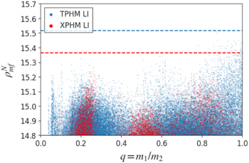
Figure 7. Comparison of network matched-filter S/N as a function of mass ratio q = m1/m2, for our default IMRPhenomTPHM and IMRPhenomXPHM results obtained with LALINference MCMC. The dashed lines indicate the maximum S/N values. Only values greater than 14.8 are shown.
Download figure:
Standard image High-resolution imageIn order to better explore the regime of very unequal masses, we have performed IMRPhenomTPHM runs with restricted mass-ratio priors, both with LALInference and with pBilby. In Figure 8 one can see that results are consistent with not finding particular support for another mode below the one at q ∼ 0.2. The full-prior run is poorly sampled in this region, with only 3.6% of samples below q = 0.15, so the small peak at q = 0.06 is probably an artifact from insufficient resolution in this region, and it is not recovered by the restricted runs. The maximum S/N recovered by the restricted runs is also lower than the S/N recovered by the full run near-equal masses.
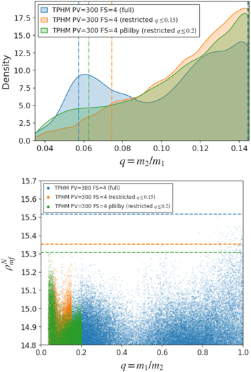
Figure 8. Top: posterior distributions for the mass ratio, comparing the standard IMRPhenomTPHM results with the full-prior range (blue) against restricted-prior results obtained with LALInference (orange) and pBilby (green). Bottom: S/N values as a function of mass ratio for the same three full-prior and restricted-prior runs. Dashed lines correspond to the maximum S/N value from each run. Only values greater than 14.5 are shown.
Download figure:
Standard image High-resolution imageWe have also checked that results are robust for different IMRPhenomTPHM versions, as can be seen in Figure 9. As discussed in the Appendix, the bimodality is not recovered when using only the dominant ℓ ≤ 2 spherical harmonic modes, but is robust under inclusion of different subsets of the higher-order modes implemented in IMRPhenomTPHM. Therefore, we overall find clear evidence for a bimodal mass-ratio posterior with a secondary unequal-mass-ratio peak near Q ∼ 5, but while there is also nonvanishing posterior support reaching to even more extreme ratios, we find no clear evidence for a third peak as originally reported in Nitz & Capano (2021). These results are consistent with Capano et al. (2021) and Mehta et al. (2021).

Figure 9. Comparison of LALInference results with different precession versions of the IMRPhenomTPHM model.
Download figure:
Standard image High-resolution image5.5. Spin and Precession
In terms of spins, one can see in Figure 3 that while IMRPhenomXPHM recovers a posterior that is approximately symmetric around χp = 0.5, IMRPhenomTPHM strongly favors high values of χp. For χeff, the IMRPhenomXPHM posterior is bimodal, with peaks close to χeff = 0 and at large negative values, while the IMRPhenomTPHM posterior is broad but unimodal with the median close to small positive values. This is reflected also in the position of the  points from the posteriors: while for IMRPhenomTPHM results, both with pBilby and LALInference,
  lies at low positive χeff and high χp ≥ 0.8, for IMRPhenomXPHM, the
  is located around χp ∼ 0.5, and its χeff is large and negative.
Another thing to notice in relation to Figure 3 is that adding precession does not seem to significantly affect the distance–θJN joint distribution for IMRPhenomXPHM with respect to IMRPhenomXHM, while for the time-domain IMRPhenomT model, family precession indeed helps to better constrain the posteriors. This is supported by the Bayes factors for the precessing hypothesis (computed from the difference in log signal-to-noise Bayes factors between precessing and non-precessing results) shown in Table 4, where the time-domain models show stronger support for precession than the frequency-domain models.
Table 4. Comparison of Bayes Factors between Precessing and Non-precessing Approximants
TPHM vs THM ( ) ) | TPHM vs THM ( ) ) | XPHM vs XHM | TPHM vs XHM | NRSur7dq4 (LVC) | |
|---|---|---|---|---|---|
| Bayes factor |

|

|

|

|

|
Download table as: ASCIITypeset image
5.6. Masses and Mass Gap
In Table 5 we show the posterior probabilities for the component objects of the source of GW190521 being inside the PISN gap. The exact boundaries of this gap are not known exactly and depend in a highly nontrivial way on nuclear reaction rates and several aspects of stellar dynamics. For simplicity, we will provide probabilities computed assuming a gap either in the range [50, 120] M⊙ (Woosley 2017) or, following more recent estimates (Woosley & Heger 2021), in the range [70, 161] M⊙ (we report results for the latter case in parentheses). Shifting the estimated boundaries toward higher masses increases (decreases) the probability of the heavier (lighter) component lying in the gap; it also drastically decreases the probability of both masses being in the mass gap.
Table 5. Probabilities of Component Objects to Be in the PISN Mass Gap, Assumed to Be Either in the Range [50, 120] M⊙ or in [70, 161] M⊙ (in Parentheses)

|

|

|

| |
|---|---|---|---|---|
| TPHM PV = 300 FS = 4 ℓ ≤ 3 | 0.672(0.919) | 0.843(0.612) | 0.663(0.612) | 0.852(0.919) |
| TPHM PV = 300 FS = 4 ℓ ≤ 4 | 0.666(0.872) | 0.715(0.415) | 0.646(0.415) | 0.736(0.872) |
| TPHM PV = 300 FS = 4 ℓ ≤ 5 | 0.741(0.916) | 0.782(0.460) | 0.719(0.460) | 0.804(0.916) |
| TPHM PV = 300 FS = 2 | 0.661(0.871) | 0.705(0.414) | 0.640(0.414) | 0.726(0.871) |
| TPHM PV = 22311 FS = 3 | 0.629(0.870) | 0.713(0.463) | 0.613(0.463) | 0.728(0.870) |
| TPHM PV = 300 FS = 4 fixed sky location | 0.648(0.807) | 0.644(0.442) | 0.625(0.442) | 0.667(0.808) |
| TPHM PV = 300 FS = 4 fixed 3D localization | 0.896(0.914) | 0.897(0.780) | 0.886(0.780) | 0.907(0.914) |
| THM | 0.993(0.997) | 0.857(0.182) | 0.856(0.182) | 0.996(0.997) |
| XPHM N&C | 0.470(0.675) | 0.372(0.048) | 0.365(0.048) | 0.477(0.675) |
| XPHM LI PV = 223 FS = 3 | 0.910(0.993) | 0.785(0.166) | 0.750(0.166) | 0.946(0.993) |
| XPHM PB 1/q PV = 223 FS = 3 | 0.681(0.923) | 0.495(0.072) | 0.474(0.072) | 0.701(0.924) |
| XPHM PB 1/q PV = 223 FS = 2 | 0.711(0.970) | 0.510(0.069) | 0.493(0.069) | 0.728(0.970) |
| XPHM PB 1/q PV = 223 FS = 0 | 0.658(0.959) | 0.479(0.067) | 0.464(0.067) | 0.674(0.959) |
| XHM LI | 0.994(0.993) | 0.847(0.125) | 0.845(0.125) | 0.997(0.993) |
Note. Numbers reported here are computed as the ratio between the posterior samples inside the gap and the total sample size. The runs denoted with 1/q use priors uniform in Q = 1/q = m1/m2, while all others use the default prior uniform in q = m2/m1; see Section 5.6 for the full discussion.
Download table as: ASCIITypeset image
We observe that IMRPhenomXPHM with a prior that is flat in component masses (run with LI) has more support for the PISN gap hypothesis, as do the non-precessing models (both IMRPhenomXHM and IMRPhenomTHM). One can see that for the IMRPhenomXPHM LI run, sampled uniform in component masses, the support for at least one component in the mass gap is greater than 90%. The alternative prior uniform in Q = 1/q enhances the high-mass-ratio region of the posterior, which typically makes both components lie outside the gap. In the runs we performed with pBilby and this prior, the support for components in the mass gap drops for IMRPhenomXPHM. With IMRPhenomTPHM, the mass-gap probabilities are generally lower than for IMRPhenomXPHM.
Hence, we conclude that inference with the non-precessing models, or with IMRPhenomXPHM and the uniform-in-q prior, prefer the hypothesis of at least one object in the PISN gap (>9:1 probability ratio), matching the original conclusions of Abbott et al. (2020b) and Abbott et al. (2020c); but IMRPhenomXPHM runs with uniform-in-Q prior and IMRPhenomTPHM inference have only mild preference (ranging from ∼2:1 to ∼3:1 depending on model version and mode content) for this scenario, allowing more readily for the "straddling" hypothesis from Fishbach & Holz (2020) of the heavier BH above and the lighter BH below the PISN gap. As seen in Table 5, results for IMRPhenomTPHM with different mode content (ℓ ≤ 3, 4, 5) are broadly consistent, except for a larger probability with ℓ ≤ 3 of having the smaller mass, or either of the two masses, in the mass gap.
5.7. Extrinsic Parameters and Electromagnetic Counterpart
The tentative association of GW190521 with the AGN flare ZTF19abanrhr (Graham et al. 2020) would be hugely impactful as the first detected electromagnetic counterpart to a BBH merger and open up cosmological applications (Chen et al. 2020; Mukherjee et al. 2020; Gayathri et al. 2020b; Finke et al. 2021). This association is however far from certain (Ashton et al. 2020; Palmese et al. 2021). Still, below we report updated association probabilities based on our new parameter estimation results. It is also illustrative to study how the GW190521 posteriors would change when factoring in knowledge of the sky location and distance of this counterpart as priors on the GW parameter estimation. To do so, we consider two scenarios: in the first, we only fix the R.A. and decl. of the source, while in the second, we also fix its luminosity distance, which can be calculated from the flare's redshift assuming a standard cosmology (Planck Collaboration et al. 2016).
First, looking back at the dL
–θJN
panel of Figure 3 for the runs with standard priors (no constraints on source location), we can see that while none of the models are able to break the hemisphere degeneracy, IMRPhenomTPHM results are able to better constrain a particular inclination in each hemisphere, albeit some bimodality in each hemisphere is also present. Similarly, IMRPhenomTPHM appears to deliver a better constraint on the luminosity distance than IMRPhenomXPHM, for which there are also hints of bimodality in the posterior. We note also that the  sample of the IMRPhenomXPHM posterior has a lower luminosity distance than that of the IMRPhenomTPHM posterior, and that these results are consistent between LALInference and pBilby runs.
Switching to IMRPhenomTPHM runs with counterpart-informed priors, in Figure 10 we present the results for masses and spins. Fixing either the 2D sky location or the full 3D localization to those of the AGN flare, the support at mass ratio Q greater than 5 is enhanced in both cases. However, fixing the 3D localization also constrains the mass posteriors more overall, while fixing only the 2D sky location mostly extends support to higher Q (lower q). The 2D-fixed prior produces a slightly bimodal posterior in χeff that is however broadly consistent with that from the standard prior, while the run with fixed 3D localization shifts the posterior mode of χeff toward 0. For the precessing spin parameter χp, fixing only the sky position has no noticeable effect, while fixing the 3D localization shifts the recovered posterior distribution to milder values. It is also worth noticing that fixing the 3D localization increases the probability for the companions to be inside the PISN mass gap (see Table 5) with respect to the standard run, while fixing only the sky location prior does not seem to have an effect on this. We also report the Bayes factors for these fixed-prior runs over the default runs in Table 6, which are quite high, but require a full analysis of the actual association probability to interpret.

Figure 10. Results for the standard runs with uninformative sky localization and distance priors compared with runs where either the 2D sky location or the full 3D localization are fixed to those of the tentative AGN counterpart, for the IMRPhenomTPHM default version with LALInference.
Download figure:
Standard image High-resolution imageTable 6. Comparison of Bayes Factors for the Runs with Either 2D Sky Location or Full 3D Localization (Sky Position Plus Luminosity Distance) Fixed to the AGN Counterpart Candidate (Graham et al. 2020), Against the Default Runs with Unconstrained Localization Priors
| BF Fixed Sky Location | BF Fixed 3D Location | |
|---|---|---|
TPHM 
|

|

|
TPHM 
|

|

|
XPHM 
|

|

|
Note. While these are quite high, it is important to take into account a full analysis of the multi-messenger coincidence significance, see the text and Table 7.
Download table as: ASCIITypeset image
To quantify this probability of a physical association between the GW and electromagnetic (EM) signals, in Table 7 we show the results from performing the same multi-messenger coincidence significance analysis as presented in Ashton et al. (2020; and using their public code), based on the localization overlap. We give results for the posterior overlap integrals for the sky location ( ), for the distance alone (
 ), and for the combined 3D localization (
 ). Assuming the same prior odds as in Ashton et al. (2020), based on the reported number of flares similar to ZTF19abanrhr in the ZTF alert stream, we compute the odds
  for the coincident hypothesis. The resulting odds vary by a factor ∼2 between runs with IMRPhenomXPHM and different versions of IMRPhenomTPHM (precession prescriptions, final-spin versions, and mode content) and overall show mild preference for association. However, our results are consistent with the findings of Ashton et al. (2020), with the highest
  we find at the same level as that reported for a run with the SEOBNRv4PHM model in Ashton et al. (2020). Essentially, despite the high Bayes factors, the evidence is insufficient to confidently associate the events. For further illustration, Figure 11 shows the position of ZTF19abanrhr compared with the sky location posterior density for GW190521 recovered by our default IMRPhenomTPHM run.

Figure 11. Position of the AGN flare ZTF19abanrhr (Graham et al. 2020) compared with the sky location posterior density for GW190521 recovered by our default IMRPhenomTPHM run.
Download figure:
Standard image High-resolution imageTable 7. Posterior Overlap Integrals and Odds for the Association between GW190521 and ZTF19abanrhr (Graham et al. 2020), Following the Method from Ashton et al. (2020)

|

|

|

| |
|---|---|---|---|---|
TPHM PV = 300 FS = 4 
| 4.7 | 17 | 140 | 6 |
TPHM PV = 300 FS = 4 
| 5.1 | 30 | 140 | 12 |
TPHM PV = 300 FS = 2 
| 4.6 | 33 | 140 | 12 |
TPHM PV = 22311 FS = 3 
| 4.7 | 20 | 110 | 7 |
| XPHM LI PV = 223 FS = 3 | 3.8 | 19 | 110 | 6 |
Download table as: ASCIITypeset image
6. Conclusions
In this paper we have reanalyzed GW190521, the highest-mass GW event yet detected, with two recently developed waveform models. First is IMRPhenomXPHM, which is a successor to previous frequency-domain IMRPhenom models, which have become standard tools in GW data analysis, but are not an optimal choice for very high-mass events, where S/N primarily comes from the ringdown to the final Kerr black hole, as can be seen in Figure 4. Second, we have used the new time-domain IMRPhenomTPHM model, which improves over IMRPhenomXPHM in how it treats precession, in particular regarding the ringdown, and which recovers a higher S/N (however consistent within statistical errors) and signal-to-noise Bayes factor (see Table 2). Our overall results are broadly consistent with the original LVC analysis (Abbott et al. 2020b, 2020c), in the sense that the inferred source parameters are consistent at 90% credible intervals. We confirm the complicated multimodal posterior structure as first reported by Nitz & Capano (2021), including support for more unequal-mass ratios, but with different statistical significance of the peaks compared to what has been found in Nitz & Capano (2021).
Before summarizing some more of our findings, we stress that our analysis is not the final answer on this uniquely challenging event either: ongoing efforts of several research groups are expected to improve accuracy in the regime considered here on the timescale of the next observation run (O4), and to advance the understanding of systematic errors of precessing waveform models. Toward the goal of constructing accurate generic waveform models, different approaches set complementary priorities. The phenomenological and EOB waveform modeling programs have developed models that cover a large portion of the quasi-circular parameter space region of compact binaries, including large mass ratios and long waveforms that can be used for low masses. Precessing NR waveforms (in particular ones that are long enough to cover a broad frequency range) are computationally expensive, and the parameter space is being explored slowly. For this reason, the phenomenological and EOB waveform programs have employed NR waveforms to test models, but have not relied on them to calibrate the first generations of precessing models with broad coverage. The program to construct surrogate models that interpolate numerical waveforms has followed a complementary strategy, and has focused on a smaller parameter region in mass ratio, spin, and waveform length, where NR waveforms are available. This range is expected to expand soon, in particular to higher mass ratios, while phenomenological and EOB models are foreseen to incorporate more information from NR simulations. A first step in this direction has recently been taken in Hamilton et al. (2021), which describes calibrating a precessing extension of IMRPhenomD (Husa et al. 2016; Khan et al. 2016; which describes the dominant ℓ = ∣m∣ = 2 modes of non-precessing systems) in the Fourier domain for single-spin systems, neglecting the dependence on the spin orientation, which is responsible for the large recoils that are possible in precessing systems (Bruegmann et al. 2008). Extending such calibrations to IMRPhenomXPHM and IMRPhenomTPHM is expected before or during O4, and the quality of such calibrated models will crucially depend on the number and quality of available NR simulations.
One way of analyzing systematic errors would be to perform injection studies, where NR waveforms are injected into synthetic noise and then the bias of the recovered parameters can be studied. For GW190521-like signals, one of the challenges of such a study is the lack (or sparsity) of suitable NR waveforms across the relevant part of parameter space, including very unequal masses. Another one is that, especially for signals with strong precession, the results may significantly depend on the extrinsic parameters chosen for the injection, which will increase the computational cost and difficulty of interpretation for such studies.
Also, it will be interesting to repeat our analysis with other currently available time-domain waveform models that also cover large mass ratios Q and can therefore be used to test posterior support in that region. A forthcoming study (Kumar Mehta et al. 2021) will present a similar reanalysis of GW190521 with the SEOBNRv4PHM model, which will allow for a direct comparison with our results.
Meanwhile, the consistency we observe between two independent sampling codes, pBilby using nested sampling (Ashton et al. 2019; Smith et al. 2020) and LALInference (Veitch et al. 2015) using MCMC sampling, gives us confidence in our results, which also appear to be robust under changes of mass priors. We have also exploited the flexibility of the IMRPhenomXPHM and IMRPhenomTPHM models to check the influence of different modeling prescriptions and choices of spherical harmonic mode content on parameter estimation, finding that posteriors are generally robust against changes in the models' internal options. In particular, we focused on the final-spin approximation, which is crucial for the ringdown regime. We have also discussed caveats when considering  points in parameter space, pointing out that maximum likelihood is typically poorly resolved by the posterior samples from Bayesian parameter estimation algorithms.
While keeping in mind that future waveform models will provide further insight into the properties of GW190521, with this study we already provide improved parameter estimation results for the source of this event. One of our central results is to confirm the multimodal nature of the posterior found in Nitz & Capano (2021), with strong support for two peaks at near-equal mass ratios and at Q ∼ 5. However, we do not find significant support for an intermediate-mass-ratio merger with mass ratios of ten or higher, consistent with other recent results by Capano et al. (2021) and Mehta et al. (2021). We do not exclude further modes at higher Q, but we do not expect them to be significant based on our findings, and most importantly, current waveform models are at this time significantly less reliable for mass ratios below our cutoff of q = 0.035 (Q = 28.57). We also provide updated probabilities of component masses being located in the PISN mass gap, in general confirming the preference of the original LVC analyses for at least one component inside the gap. However, this occurs with IMRPhenomTPHM results reducing the preference against a "straddling" binary configuration with one component below and one above the mass gap, and of associating GW190521 to the potential electromagnetic counterpart (Graham et al. 2020).
We thank Gregory Ashton, Colm Talbot, and Rory Smith for valuable discussions about GW parameter estimation with Bilby. This work was supported by European Union FEDER funds, the Ministry of Science, Innovation and Universities and the Spanish Agencia Estatal de Investigación grants PID2019-106416GB-I00/AEI/10.13039/501100011033, RED2018-102661-T, RED2018-102573-E, FPA2017-90687-REDC, Comunitat Autonoma de les Illes Balears through the Direcció General de Política Universitaria i Recerca with funds from the Tourist Stay Tax Law ITS 2017-006 (PRD2018/24), and Conselleria de Fons Europeus, Universitat i Cultura, i Fons Social Europeu, EU COST Actions CA18108, CA17137, CA16214, and CA16104. Generalitat Valenciana (PROMETEO/2019/071). D.K. is supported by the Spanish Ministerio de Ciencia, Innovación y Universidades (ref. BEAGAL 18/00148) and cofinanced by the Universitat de les Illes Balears. M.C. acknowledges funding from the Spanish Agencia Estatal de Investigación, grant IJC2019-041385. The authors acknowledge and thank the computer resources at MareNostrum and the technical support provided by Barcelona Supercomputing Center (BSC) through grant Nos. AECT-2020-2-0015, AECT-2020-1-0025, AECT-2019-3-0020, AECT-2019-2-0010, AECT-2019-2-0017, and AECT-2019-1-0022, from the Red Española de Supercomputación (RES). The authors also acknowledge the computational resources at the cluster CIT provided by LIGO Laboratory and supported by National Science Foundation grant Nos. PHY-0757058 and PHY-0823459. This research has made use of data obtained from the Gravitational Wave Open Science Center (LIGO Scientific Collaboration & Virgo Collaboration 2020b), a service of LIGO Laboratory, the LIGO Scientific Collaboration and the Virgo Collaboration. LIGO is funded by the U.S. National Science Foundation. Virgo is funded by the French Centre National de Recherche Scientifique (CNRS), the Italian Istituto Nazionale della Fisica Nucleare (INFN) and the Dutch Nikhef, with contributions by Polish and Hungarian institutes.
Appendix: Analysis of Harmonic Content
For short-duration signals like GW190521, the inclusion of different harmonics in the signal templates can be even more crucial than in the lower-mass case when the inspiral is also observable, helping to break possible degeneracies between parameters and to obtain more information from the signal. To test the effect of including different sets of harmonics, in Figure 12 we compare the main parameters of the signal for runs performed with different harmonic content, going from ℓ ≤ 2 up to ℓ ≤ 5. We can observe how the recovered posterior densities tend to converge as more harmonics are included, resulting in a very similar distribution for ℓ ≤ 4 and ℓ ≤ 5. This finding justifies in part our choice of performing the main runs of this work for the subset ℓ ≤ 4. Going beyond ℓ ≤ 5, future work will be required to study the impact of harmonics that are not included in our waveform models.
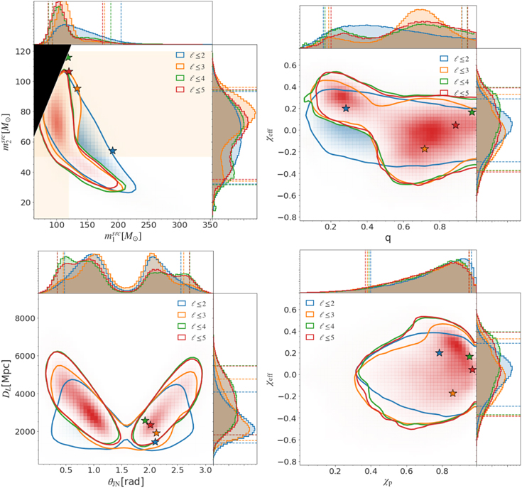
Figure 12. Comparison of posterior distributions obtained with IMRPhenomTPHM with different spherical harmonic mode content ℓ ≤ 2, 3, 4, and 5.
Download figure:
Standard image High-resolution imageA rough quantitative estimate of the importance of higher modes can be obtained by computing the optimal S/N contributed by each harmonic. The optimal S/N for one mode can be defined as

where 〈, 〉 refers to the usual noise-weighted inner product, and hlm denotes the contribution of a given mode to the strain measured by the detector. We compute the S/N contribution of each harmonic employing the same PSDs we use for parameter estimation throughout this paper. In order to cleanly separate between different modes in the inertial frame, we perform the calculation using the aligned-spin version of the models, namely IMRPhenomXHM and IMRPhenomTHM. The source parameters are taken from the posterior samples of the same IMRPhenomTPHM LALInference run (corresponding to the red curves of Figure 3). We present our results in Figure 13: based on the S/N contribution of each harmonic, one would expect the largest impact on posteriors from the inclusion of the (3,3) mode. This conclusion is consistent with the results of a full Bayesian inference analysis outlined above, where the results for ℓ ≤ 2 are very different from the more complete runs, but changes from ℓ ≤ 3 to ℓ ≤ 4 are more moderate, and the ℓ ≤ 4, ℓ ≤ 5 results are very similar.
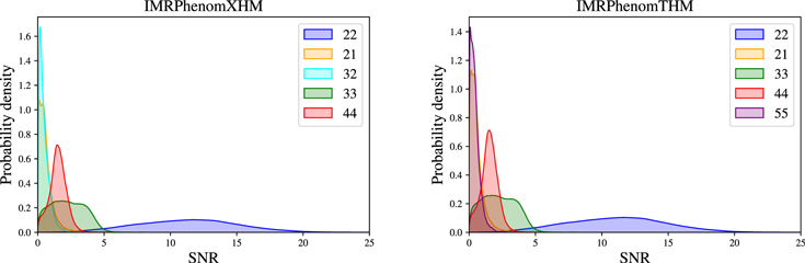
Figure 13. Optimal S/N corresponding to different harmonics, computed on the same posterior samples from our default LALInference runs for IMRPhenomXHM (left panel, with PV = 223, FS = 3 settings) or IMRPhenomTHM (right panel, with PV = 300,FS = 4 settings).
Download figure:
Standard image High-resolution image