


Abstract
Magnetic field line reconnection is a universal plasma process responsible for the conversion of magnetic field energy to plasma heating and charged particle acceleration. Solar flares and Earth's magnetospheric substorms are two of the most investigated dynamical systems where global magnetic field reconfiguration is accompanied by energization of plasma populations. Such a reconfiguration includes formation of a long-living current system connecting the primary energy release region and cold dense conductive plasma of the photosphere/ionosphere. In both flares and substorms the evolution of this current system correlates with the formation and dynamics of energetic particle fluxes (although energy ranges can be different for these systems). Our study is focused on the similarity between flares and substorms. Using a wide range of data sets available for flare and substorm investigations, we qualitatively compare the dynamics of currents and energetic particle fluxes for one flare and one substorm. We show that there is a clear correlation between energetic particle precipitations (associated with energy release due to magnetic reconnection seen from riometer and hard X-ray measurements) and magnetic field reconfiguration/formation of the current system, whereas the long-term current system evolution correlates better with hot plasma fluxes (seen from in situ and soft X-ray measurements). We then discuss how data sets of in situ measurements of magnetospheric substorms can help interpret solar flare data.
Export citation and abstract BibTeX RIS
1. Introduction
Magnetic field energy release and the associated acceleration and heating of charged particles are common properties of powerful plasma phenomena such as flares in the solar atmosphere and substorms of Earth's magnetosphere. This similarity has been underlined almost from the beginning of flare investigation (e.g., Obayashi 1975; Akasofu 1979; Syrovatskii 1981) and is still actively discussed (Terasawa et al. 2000; Reeves et al. 2008; Birn et al. 2017; Oka et al. 2018; Sitnov et al. 2019a). The basic elements of flares and substorms include formation of spatially localized regions with strong electric current density (sometimes in the form of current sheets; see Akasofu 1979; Parker 1994; Birn & Priest 2007; Rappazzo & Parker 2013), magnetic field line reconnection (Priest & Forbes 2000; Gonzalez & Parker 2016), energization of charged particles (Aschwanden 2002; Zharkova et al. 2011; Birn et al. 2012; Oka et al. 2018), and their precipitation to the much denser photosphere/ionosphere (see comparisons in, e.g., Haerendel 2009, 2012) that is associated with a wide spectral range of emissions. Despite their general overall similarity, the plasma parameters and spatial scales of solar flares and Earth's magnetospheric substorms are significantly different. This complicates direct comparisons but still leaves room to search for phenomenological similarities between these two systems.
One of the key elements of magnetospheric substorms is the formation of a new type of current system that connects the strong cross-field currents of the hot (≤1 keV electrons and ≤5 keV ions) rarefied (collisionless) magnetotail with the field-aligned currents of the cold (∼eV) dense (resistive) ionosphere (e.g., Kepko et al. 2014; Ganushkina et al. 2015). The development and dynamics of this current system (so-called substorm current wedge) occur on the substorm global timescale, whereas spatially localized particle energizations and precipitations (up to a few hundred keV) may intensify on much smaller timescales. A combination of multispacecraft in situ measurements in the magnetotail (e.g., see reviews by Petrukovich et al. 2015; Sitnov et al. 2019a), ground-based measurements of magnetic fields and various emissions (see, e.g., Keiling 2009; Nishimura et al. 2020), and empirical models (e.g., Andreeva & Tsyganenko 2019; Sitnov et al. 2019b; Stephens et al. 2019) describes most of the elements of this current system and the relations of these elements to such processes as particle energization and precipitation. But can this information be somehow useful for the investigation of solar flares that are mostly probed with remote observations and various reconstruction techniques? This study aims to address this question by comparing two events—one moderate magnetospheric substorm and one moderate (M-class) solar flare. We focus on two aspects of flares/substorms: (i) dynamics of magnetic field and electric currents, and (ii) their correlation with charged particle energization.
Such a comparison of currents and magnetic fields for flares and substorms has become possible only recently, with a new observational data set of solar physics—high-cadence (135 s) photospheric vector magnetograms by the Helioseismic and Magnetic Imager (HMI) on board the Solar Dynamics Observatory (SDO; Scherrer et al. 2012; Centeno et al. 2014; Hoeksema et al. 2014). Having lower signal-to-noise ratio than 12-minute averaged magnetograms, these high-cadence magnetograms still provide sufficiently accurate measurements for long (>2 minutes) and intense (magnetic field perturbations higher than ≈300 G) events (Sun et al. 2017; Sharykin et al. 2020).
We start with a detailed description of available data sets in Section 2. This description continues our introduction, because we include technical details of measurement techniques and data with their comparison for flares and substorms. Materials and interpretations of the spacecraft and ground-based measurements for a selected substorm are provided in Section 3.1. Materials and interpretations of the data set available for the flare investigation are provided in Section 3.2. Finally, we discuss the results obtained and provide a general perspective of using the magnetospheric concepts/data for investigating solar flares in Section 4.
2. Data Sets and Methods for Substorms
In this section we provide the detailed description of data sets related to substorm investigations and point out analogies between these data sets and those available for the solar flare. The detailed discussion of the solar flare data set is given in Section 3.2. To describe available data sets of in situ spacecraft measurements, we show spacecraft locations relative to the magnetic field line configuration in Earth's magnetotail (see Figure 1(a)). This configuration is from the empirical magnetic field model (Tsyganenko 2002), and we consider an interval before reconnection onset (before energy release). Two Acceleration, Reconnection, Turbulence and Electrodynamics of the Moon's Interaction with the Sun (ARTEMIS) probes, P1 and P2 (Angelopoulos 2011), are located in the deep tail (around the Moon; radial distance from Earth is r ∼ 60RE, where RE is Earth's radius) and mainly observe the outflow from reconnection that is expected to form at r ≲ 30RE (the statistically most probable region; see Genestreti et al. 2014). In the context of solar flares such measurements are some analog of measurements of the solar wind outflow and mass ejection coming from the flare, but this analogy should take into account that ARTEMIS is much closer to the reconnection side than any direct measurements of plasma outflow from flares. ARTEMIS is equipped with fluxgate magnetometers (Auster et al. 2008), electrostatic analyzers (ESA; McFadden et al. 2008), solid-state telescopes (SSTs; Angelopoulos et al. 2008b), and wave instruments (Bonnell et al. 2008; Cully et al. 2008; Le Contel et al. 2008). We will analyze magnetic field vector, ion and electron spectra (<30 keV from ESA and 50–500 keV from SST; see Turner et al. 2012 for details of ESA-SST cross-calibration), and ion velocity vector provided in 4 s (spacecraft spin) resolution.

Figure 1. Panel (a) shows spacecraft locations on top of magnetic field lines reconstructed from the empirical magnetic field model (Tsyganenko 2002). Panel (b) shows AE and Sym − H geomagnetic indices. Panel (c) shows solar wind velocity vx and magnetic field Bz .
Download figure:
Standard image High-resolution imageCloser to Earth, in the magnetotail, four spacecraft from the Magnetospheric Multiscale (MMS) mission (Burch et al. 2016a) measure reconnection outflow moving toward Earth (see Figure 1(a)). The very small separation of these spacecraft makes their measurements almost identical to one another in our event (however, such small separation is extremely useful for the investigation of fine structure in the reconnection region; e.g., Burch et al. 2016b; Torbert et al. 2018; Turner et al. 2021). One of the possible and prominent observational manifestations of the reconnection outflow in solar flares are the supra-arcade downflows (SADs; see discussion of this analogy in Sitnov et al. 2019a; Xue et al. 2020). In a more general sense, the MMS data set resembles estimates of outflow velocities and emissions from the energy release region in the solar corona that are obtained for some flares with spatially and/or spectrally resolved observations in the soft X-ray and extreme-ultraviolet (EUV) ranges (e.g., Hara et al. 2011; Takasao et al. 2012; Kumar & Cho 2013; Su et al. 2013; Srivastava et al. 2019). We use four instruments on board MMS: fluxgate magnetometer (Russell et al. 2016), Fast Plasma Instrument (FPI; Pollock et al. 2016), Energetic Ion Spectrometer (EIS; Mauk et al. 2016), and Fly's Eye Energetic Particle Sensor (FEEPS; Blake et al. 2016). These instruments provide magnetic field vectors (64 Hz are routinely available), ion and electron spectra (<30 keV from FPI, 50–500 keV from EIS and FEEPS), and ion velocity vectors with 5 s (spacecraft spin) resolution.
At high geomagnetic latitudes and closer distances to Earth the Exploration of energization and Radiation in Geospace (ERG, Arase) spacecraft (Miyoshi et al. 2018b) measures the flux of particles moving along magnetic field lines from the equatorial region (see Figure 1(a)), including the equatorial region of the reconnection outflow, because particles quickly reach ERG along magnetic field lines. Despite its close location to Earth, the local loss-cone size for ERG is still pretty small (several degrees), and most of the observed particles are trapped, i.e., will be reflected by Earth's strong magnetic field and move back to the equator. These ERG measurements may be considered as some sort of analog of emissions from the heated magnetic loops after flare energy release. In particular, the precipitation of accelerated electrons (≳30 keV) and ions (≳10 MeV nucleon−1) into the dense layers of the solar atmosphere is observed as the sources of hard X-ray and gamma-rays, respectively, at the footpoints of flare loops as shown by, e.g., the RHESSI data (Lin et al. 2002; Hurford et al. 2006; Krucker et al. 2011). Accelerated particles and conductive heat fluxes from the energy release site in the corona propagate down along magnetic field lines and heat the plasma in the transition layer and the chromosphere. The result is an emission in the UV and optical ranges (e.g., in Hα)—the so-called flare bright kernels and flare ribbons (e.g., see the review by Fletcher et al. 2011). We use four instruments on board ERG: the fluxgate magnetometer (MGF; Matsuoka et al. 2018a, 2018b), the electron Low-energy electron sensor (LEPe; Kazama et al. 2017; Wang et al. 2018b), and the ion and electron Medium-energy particle sensors (MEPe and MEPi; Yokota et al. 2017, 2018; Kasahara et al. 2018a, 2018b). These instruments provide magnetic field vectors and ion and electron spectra (<20 keV from LEPe, 10–180 keV q−1 from MEPi, and 7–87 keV from MEPe) with 8–16 s resolution.
At the equator, close to Earth, the Geostationary Operational Environmental Satellite (GOES) spacecraft measures magnetic field perturbations. For sufficiently strong magnetospheric substorms GOES generally detects injections of energetic particles into Earth's inner magnetosphere, but for the moderate event under consideration GOES only measures magnetic field perturbations (with the fluxgate magnetometer; see Singer et al. 1996). We use this data set, which has a time resolution of 1 minute.
These four missions (ARTEMIS, MMS, ERG, and GOES) provide in situ magnetic field and plasma measurements for our event, and these data are well supplemented by ground-based measurements. Magnetic field lines from the magnetotail for this event are projected to the northern USA/Canada, where a very large network of ground-based magnetometers operates (Engebretson et al. 1995; Mann et al. 2008; Russell et al. 2008; Lam 2011). Such magnetometers provide the magnetic field vector with 0.5–10 s resolution, and such fields show development of the ionospheric current system and ionosphere–magnetosphere currents (e.g., Kepko et al. 2014; Ganushkina et al. 2015). Owing to the good coverage of ground-based magnetometers, these measurements can be combined into the general data set for reconstruction of currents on the ionosphere level (Amm & Viljanen 1999). We use the database of such currents provided by Weygand et al. (2011, 2012) and containing transverse (to Earth's surface) current densities and field-aligned (∼normal to the surface) current with a time resolution of 10 s. This data set is the direct analog of currents and magnetic field on the photosphere level reconstructed for the solar flares (e.g., Janvier et al. 2014; Musset et al. 2015; Sharykin et al. 2020; Zimovets et al. 2020).
Integral characteristics of ground-based magnetic field perturbations provide the geomagnetic indices, e.g., Sym − H and AE. The Sym − H index, which is a 1-minute version of the 1 hr Dst index (Wanliss & Showalter 2006), quantifies longitudinally symmetric geomagnetic disturbances at midlatitudes and serves as a measure of intensity of currents carried by hot (≥5 keV) and energetic (<100 keV) ions injected deep into the inner magnetosphere (i.e., earthward from the GOES location in Figure 1). Such currents are going around Earth and are called ring currents (Daglis et al. 1999). Essentially, Sym − H describes the power of geomagnetic storms (e.g., Gonzalez et al. 1994), much more intense perturbations than a substorm under consideration. Figure 1(b) shows that Sym − H index is quite small and there are no energetic ion injections penetrating sufficiently close to start drifting around Earth for our event. However, ASym − H index (which characterizes asymmetric magnetic field perturbations due to energetic ion enhancements at the nightside) increased from 3 to 6 nT for our event (not shown). This quite significant change indicates energetic ion injection at the nightside, where such injections can feed partial ring current (Liemohn et al. 2016; Sitnov et al. 2019b).
The Auroral Electrojet index, AE, measures auroral zone (where most of hot (∼1 keV) electrons from the magnetotail are precipitating, i.e., where a new current system connects the magnetosphere and ionosphere currents) magnetic field perturbations and quantifies the substorm power (e.g., Kamide & Rostoker 2004). Figure 1(b) shows AE increase starting from ∼03:00, when the substorm onset has been observed by spacecraft in the magnetosphere (see below). We show the AE averaged over all auroral zone stations around Earth (the Kyoto AE), whereas the AE calculated for the subset of stations projected to the substorm location is even larger and reaches ∼300 nT in the peak at ∼03:30. Such an AE index magnitude corresponds to moderate substorms.
Ground-based magnetometer measurements are supplemented by all-sky imager measurements at the South Pole (Ogawa et al. 2020b). The imager was in the premidnight sector (23.5 MLT at 3 UT, −74 deg MLAT), in the same sector as the satellites in the magnetosphere. The camera provides sufficiently high spatial (∼1 km) and temporal resolution (1 and 4 s at 557.7 and 630.0 nm wavelength, respectively) to detect emissions related to electron precipitations from the substorm magnetotail (Chu et al. 2020). The emission heights at 557.7 and 630.0 nm are determined to be 110 and 230 km altitude, respectively. Auroral emissions at 557.7 and 630.0 nm are sensitive to precipitating electrons above and below ∼1 keV, respectively, which cover a similar energy range to electrons producing soft X-ray emissions in solar flares.
In addition to ground-based magnetometers and all-sky cameras, this study makes use of data (1 s resolution) from a 30 MHz riometer located in Iqaluit (IQA), Canada. This riometer is a passive sensor employing a single zenith-pointed antenna and measures the radio noise intensity from extraterrestrial sources to characterize the opacity of the ionosphere (Browne et al. 1995; Danskin et al. 2008). Deviations of the received signal voltage from the voltage expected on a quiet day are used to derive signal absorption in decibels (dB). The riometer voltage is directly related to energetic electron precipitation to the cold dense ionosphere (riometers mainly respond to precipitations of energies above a few tens of keV; see, e.g., Gabrielse et al. 2019). Thus, the riometer data set is the direct analogy of the bremsstrahlung hard X-ray emission produced by precipitating energetic (tens of keV) electrons in solar flares (e.g., Brown 1971; Syrovatskii & Shmeleva 1972; Kontar et al. 2011).
If geomagnetic indices monitor the dynamics of current systems in the magnetotail after reconnection onset, the drivers of this onset are generally associated with the solar wind, monitored by spacecraft at L1 (Acuña et al. 1995; King & Papitashvili 2005; Koval et al. 2013). The main solar wind characteristics affecting magnetotail dynamics and reconnection are plasma velocity (or dynamical pressure) jumps (see, e.g., Angelopoulos et al. 2020) and orientation of the Bz component of the solar wind magnetic field (see, e.g., Baker et al. 1996). Figure 1(c) shows that, for the event under consideration, the solar wind velocity is quite stable and Bz is mostly positive: there are no conditions for strongly driven reconnection, and the substorm is expected to be moderate.
3. Currents and Energetic Particle Fluxes
We start with a discussion of the physical processes and their observational evidence in the magnetosphere substorm: from in situ spacecraft observations to the ground-based magnetic field measurements. Then, we present the solar flare observation and compare it to the substorm observations.
3.1. Substorm
Figures 2(a)–(c) shows ARTEMIS and MMS measurements of plasma flows along the x-direction and the Bz magnetic field component (see Figure 2(d) for the geometry of the reconnected current sheet in Earth's magnetotail). For the main event at 03:00 UT, MMS detected clear evidence of reconnection. MMS first observed vx > 0 and Bz > 0 at ∼03:00 UT. Although at this time MMS was still relatively away from the equatorial plane (Bx > 15 nT), it started to observe energetic, >10 keV ions (Figure 2(e)) associated with vx > 0 (such earthward plasma flows and energetic ion populations are usually considered to originate from reconnection). The appearance of vx > 0 was associated with an increase of Bz > 0, indicating that the reconnection started on the tailward side of MMS. At 03:06 UT, MMS started to detect hot plasma (Figure 2(e)), further supporting our interpretation of magnetic reconnection, although its bulk velocity (vx ) was not so high and it fluctuated between earthward (positive) and tailward (negative) until 03:45 UT (Figure 2(a)).
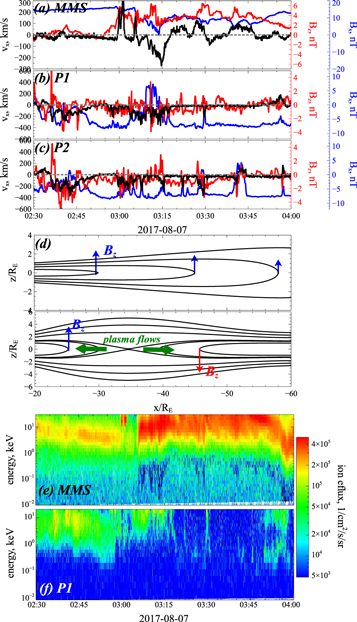
Figure 2. (a) MMS and (b, c) ARTEMIS measurements of plasma flow velocity vx (black), magnetic field Bz (red), and magnetic field Bx (blue). Panel (d) is a schematic of the magnetotail current sheet configuration before (top) and after (bottom) reconnection. Panels (e) and (f) show ion spectra measured by MMS and ARTEMIS P1.
Download figure:
Standard image High-resolution imageAs the earthward flow at 03:00 at MMS is associated with the quite large Bx ∼ 15 nT, it can be interpreted as a field-aligned flow from the reconnection side located beyond ∼ − 35RE. The next earthward flow at ∼03:06 UT is observed around the equator (Bx < 5 nT) and is associated with a significant increase of fluxes of hot (>10 keV) ions (see Figure 2(e)). This is earthward plasma flow moving from the reconnection region and transporting magnetic flux (electric field Ey ∼ vx Bz /c > 0). Both ARTEMIS probes at ∼03:05 UT observed vx < 0 and Bz < 0: a tailward plasma flow moving from the reconnection region and also transporting magnetic flux (electric field Ey ∼ vx Bz /c > 0); see details in Angelopoulos et al. (2013). MMS and ARTEMIS observations suggest that the magnetic reconnection occurs right between these spacecraft, somewhere around ∼ − 35RE (see spacecraft locations in Figure 1).
ARTEMIS observations before 02:50 UT show tailward plasma flow (vx < 0, Bz < 0) indicating another reconnection event occurring before the main one, at ∼03:00–03:05 UT. However, during that time the MMS spacecraft were quite far from the equatorial plane and did not see earthward flows (vx ∼ 0 on MMS), i.e., the energy release during this reconnection event was not sufficiently strong to generate plasma flows that reconfigure the near-Earth magnetotail current sheet and expand the plasma sheet out to the MMS location. For the main event at ∼03:06 UT such flows change the magnetic field configuration of the near-Earth current sheet (∣Bx /Bz ∣ > 15 before 03:00 and ∣Bx /Bz ∣ < 2 after 03:06 on MMS), increase its thickness (so-called plasma sheet expansion; see schematic in Figure 2(d) and Baker et al. 1996; Baumjohann et al. 1999; Baumjohann 2002), and move the MMS spacecraft to the equator, where they observed vx > 0.
After ∼03:00 UT ARTEMIS observed bursts of tailward flows vx < 0, Bz < 0 for almost 40 minutes, whereas MMS observed oscillating vx and Bz . The transient nature of ARTEMIS observations is due to the transient nature of reconnection that is not steady in the magnetotail (e.g., Heyn & Semenov 1996; Semenov et al. 1992; Sitnov et al. 2009) and to vertical oscillations of the magnetotail current sheet (see Runov et al. 2005; Vasko et al. 2015) that periodically move the spacecraft closer to or farther from the equator. Oscillations of vx and Bz on MMS are of a more interesting nature and probably are somewhat analogous to quasi-periodical vertical magnetic loop oscillations observed in some solar flares (e.g., Wang & Solanki 2004; Li & Gan 2006; Russell et al. 2015). The earthward plasma flow vx > 0 transports magnetic flux to the region of strong dipole magnetic field, and the impact of this flow compresses magnetic field lines there. This drives magnetic field lines and plasma oscillations along x (see Panov et al. 2010, 2013; Wolf et al. 2018; Toffoletto et al. 2020), i.e., MMS may have observed quasi-periodical motions of magnetic field lines with vx > 0 periods associated with Bz peaks (more dipolar configuration of magnetic field lines) and vx < 0 periods associated with Bz > 0 minima (more stretched configurations of magnetic field lines).
Figure 3 shows fluxes of energetic (>30 keV) ions and electrons, as well as Bx profiles observed by MMS, ARTEMIS, and ERG. Bx profiles are included to separate temporal variations of energetic (30–100 keV) fluxes from their spatial variations: in the magnetotail ∣Bx ∣ is a proxy of the spacecraft location relative to the equator (Bx = 0). At ∼03:00 UT MMS and ARTEMIS (mainly P1, which is closer to the equator than P2) observed a rapid increase of energetic particle fluxes right after reconnection. The magnetic field topology (magnitude of Bx and strong Bx variations) and spectra of thermal (a few keV for electrons and <30 keV for ions) plasma (e.g., see Figures 2(e) and (f) and 6(c)) unambiguously show that MMS is on the closed magnetic field lines, well within the magnetotail plasma sheet (see Frank 1985; Ashour-Abdalla et al. 1996, for the detailed comparison of plasma populations observed on closed and open magnetic field lines in the magnetotail). Therefore, energetic particles (both electrons and ions with energies >30 keV) on the MMS side are trapped on these closed lines, bouncing between magnetic mirrors located near Earth, where the magnetic field well exceeds the magnetic field at the MMS location.
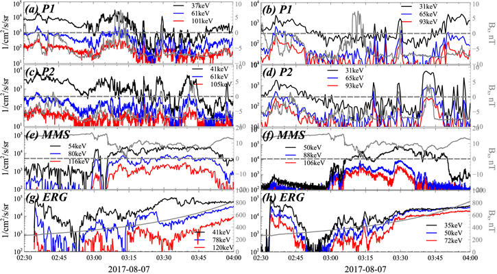
Figure 3. (a–d) ARTEMIS, (e, f) MMS, and (g, h) ERG measurements of energetic ion fluxes (left) and energetic electron fluxes (right). Each panel also shows Bx on the spacecraft (gray).
Download figure:
Standard image High-resolution imageContrary to MMS, the ARTEMIS probes in the deep tail are on open magnetic field lines. Energetic particles arriving at ARTEMIS from the reconnection region quickly escape along open field lines to the solar wind. This explains why energetic (30–100 keV) particle fluxes on ARTEMIS are much smaller than fluxes at MMS (see also Runov et al. 2018). Note that some fluctuations of fluxes on ARTEMIS are due to oscillations of the current sheet (see Bx variations) that result in ARTEMIS motion away from the equator.
At ∼03:00 UT, ERG also observed an increase of energetic (30–100 keV) particle fluxes. These energetic particles arrive at ERG along magnetic field lines. Although ERG magnetic field is much stronger than magnetic fields measured by equatorial MMS and ARTEMIS, this field is much smaller than the near-Earth surface field. The loss-cone size on ERG is about several degrees, and almost all measured fluxes are trapped, i.e., energetic particles are bouncing along magnetic field lines that are crossed by ERG. Observed flux pitch-angle distributions show that parallel and antiparallel fluxes are very similar (not shown). Prior to 03:00 UT, the MMS spacecraft were on magnetotail field lines, far from the equator (see large Bx ), and can be projected to the deep tail, where fluxes of energetic (>30 keV) particles are very low (there is no MMS observation of ∼100 keV fluxes before ∼03:00 UT). Prior to 03:00 UT, ERG was in the inner magnetosphere and projected to the near-Earth region, where energetic (>30 keV) particle fluxes can be quite high, as particles of these energies are trapped there by strong magnetic field and can survive from the previous energy release. This explains why ERG observed sufficiently large ∼100 keV fluxes even before ∼03:00 UT. The dynamics of energetic fluxes on ERG and MMS can be compared with currents and magnetic field dynamics on the ground, to establish relationships between the formation of new current systems and the energy release process.
Figure 4(a) shows locations of ground-based magnetometer stations measuring magnetic field that can be used to calculate the horizontal (shown by black arrows) and vertical (color) currents. The right side of Figure 4(a) shows two clear field-aligned currents: a downward region 1 current (blue) at high latitude and an upward region 2 current (red) equatorward of the region 1 currents. The horizontal currents are equivalent currents that are a combination of Hall and Pedersen currents where the bulk contributor is the Hall current system and the strongest currents flow from east to west between the region 1 and 2 current system (for more details see Weygand et al. 2011, 2012). The Pedersen currents connect the downward region 1 currents with the upward region 2 currents. Thus, current flows from the magnetotail along magnetic field lines, then traverses from north to south (along the ionospheric surface), and finally flows back to the magnetotail. This is the ionospheric part of the current wedge (Kepko et al. 2014) that is closed by the cross-field current in high-β magnetotail current sheet.
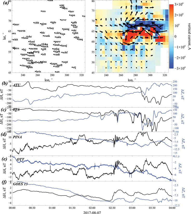
Figure 4. Panel (a) shows the location (in geographic latitude, longitude) of the ground-based stations measuring magnetic field (left), density of the transverse current (black arrows), and intensity of downward and upward vertical currents in red and blue at 03:20 UT (right). Panels (b)–(f) shows variations of horizontal H and vertical Z components of magnetic field on four ground-based stations and on the near-Earth GOES spacecraft.
Download figure:
Standard image High-resolution imageStations within the peaks of downward and upward currents detect the decrease of the horizontal (parallel to surface) magnetic field (see ΔH < 0 in Figures 4(b) and (c), ATU and IQA) and increase (for inflow)/decrease (for outflow) of the vertical component of the magnetic field (see ΔZ > 0/ΔZ < 0 in Figures 4(b) and (c)). Note that the orientation of field-aligned currents and corresponding magnetic field perturbations can vary from substorm to substorm or even within one substorm. The typical substorm current wedge system has downward field-aligned currents on the dawnside, upward field-aligned currents on the duskside, and a westward current in between. This current arrangement produces a southward magnetic field perturbation (ΔH < 0). However, for the event from Figure 4 the upward and downward currents are separated in the north–south direction. Stations located below the main inflow/outflow current region are projected to the magnetotail equator closer to Earth than the main energy release region and fast plasma flows. These stations detect an increase of the horizontal magnetic field (see ΔH > 0 in Figures 4(d) and (e), PINA and OTT), indicating that the magnetic field in the near-Earth region also increased owing to a pileup of the magnetic field transported inward by the fast plasma flows (Kokubun & McPherron 1981). Indeed, ΔH > 0 from Figures 4(d) and (e) correlates well with ΔH > 0 measured by GOES in the near-Earth magnetotail (see Figure 4(f)).
Figure 5 compares the dynamics of currents and energetic (∼100 keV) particle fluxes. We consider field-aligned (inflow and outflow) currents averaged over the regions with current magnitude larger than 103 A. To trace energetic particle fluxes in the magnetotail, we show ion and electron fluxes from ERG and MMS, whereas the enhancement of the riometer signal (reduction of signal voltage) indicates enhancements of precipitating energetic (tens of keV) electron fluxes (the riometer station is located at IQA; see Figure 4(a)). There are two moments of the current magnitude growth: at the main energy release, ∼03:00 UT, and at ∼03:15 UT. The second growth is likely due to another energy release event that is not seen by MMS but can be distinguished in ERG fluxes (see Figure 3). Both current growth intervals are associated with strong precipitations of energetic electrons detected by the IQA riometer, which observed a ∼0.6 dB increase in absorption (see Figure 5(e)). Such temporally localized precipitations are due to the combined effect of energy transport to the ionosphere by Alfvén waves (Lysak 2004; Keiling 2009) generated in the energy release region (and the following dissipation of these waves with electron field-aligned acceleration at the ionosphere/magnetosphere interface; see Lysak & Song 2003; Chaston et al. 2005, 2008; Malaspina et al. 2015) and the direct precipitation of energetic (tens of keV) electrons scattered around the equator into the loss cone by various transient electromagnetic fields generated in the energy release region (Eshetu et al. 2018; Gabrielse et al. 2019).

Figure 5. Downward (red) and upward (blue) currents from Figure 4 (averaged over the region with the current magnitude larger than 103 A) are shown together with energetic particle fluxes and precipitation signals: (a, c) electrons and ions measured by MMS, (b, d) electrons and ions measured by ERG, (e) riometer data from IQA station. Two black curves in each panel show fluxes for two energies (indicated by numbers around corresponding curves), and gray color fills the flux range between these two black curves. For panel (e) there is only one black curve showing riometer signal.
Download figure:
Standard image High-resolution imageEnergetic ion and electron fluxes at MMS do not show two peaks, but rather repeat the profiles of the currents (see Figures 5(a) and (c)). There is a clear increase of fluxes owing to electron and ion acceleration during the energy release (magnetic reconnection) occurring at ∼03:00 UT. Fluxes remain at a stable level for ∼40 minutes and decay together with the currents around ∼03:45 UT. Similar flux dynamics are shown by the ERG observations (see Figures 5(b) and (d)), but ERG also observed a second peak of energetic fluxes around ∼03:15 UT, when the currents increase. After ∼03:30 UT, ERG, moving along its highly inclined orbit, lost conjugation to the magnetotail and started observing fluxes in the inner magnetosphere that are not related to the current dynamics.
Comparison of MMS and riometer data (see Figures 5(a) and (e)) shows that precipitations of energetic (tens of keV) electrons correlate well with the intervals of current increase, whereas the slow evolution of the current is better correlated with the magnitude of equatorial energetic fluxes. Indeed, currents derived from ground-based magnetometer measurements are connected to the magnetotail cross-field currents supported by drifts of hot (∼several keV) and energetic (tens of keV) particles seen by MMS. Thus, increases of current magnitude should be due to an increase of equatorial energetic particle fluxes associated with energy releases and precipitations. In the next section we discuss the analogy of this scenario with observations of emissions and currents in the solar flare.
Ground-based measurements are not limited to magnetic fields and riometer signals but also include optical measurements by an all-sky camera at the South Pole. This data set represents 2D time-dependent pictures of emissions at different wavelengths, corresponding to precipitations of electrons of different energies. We consider red (630.0 nm) and green (557.7 nm) light emissions from ≤1 keV and ≥1 keV electron precipitations. More precisely, a higher red/green ratio indicates lower energy (red-dominant aurora has hundreds of eV energy), while a lower red/green ratio indicates higher energy (green dominant aurora has ∼10 keV energy). Note that ≥1 keV can be considered as the suprathermal part of the main electron population in the magnetotail, enhanced and scattered into the loss cone during energy release, whereas the ≤1 keV electron population comes from the thermal plasma sheet; see discussion in Runov et al. (2015) and Ganushkina et al. (2019). Figures 6(a) and (b) show keograms, which demonstrate the intensity of emissions as a function of time and latitude at a fixed longitude. We supplement keograms with spectra of <20 keV electrons measured by MMS and ERG (see Figures 6(c) and (d)). These spectra show clear heating of the main electron population (increase of energy range of the most intense fluxes from 0.2 to 2 keV before 03:00 UT to 1–10 keV after 03:00 UT; mostly seen in MMS data) at ∼03:00 UT (note that ERG captured another flux increase at ∼03:15 UT, in agreement with the two bursts of electron precipitations shown by riometers; see Figure 5(a)).
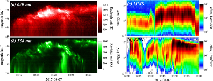
Figure 6. Panels (a) and (b) show keograms (bright emission from low latitudes corresponding to the near-Earth region) for red (corresponding to precipitations of ≲1 keV electrons) and green (corresponding to precipitations of ≳1 keV electrons) spectral lines (the color scale is Rayleigh unit (R), with 1 R = 1010 photons cm−2 s−1; see Ogawa et al. 2020a). The magnetic latitudes are in the AACGM (altitude adjusted corrected geomagnetic) coordinate system. Panels (c) and (d) show electron spectra measured by MMS and ERG spacecraft. Note that keograms show observations around the energy release moment, ∼03:20, whereas MMS and ERG spectra are shown for the entire event, from 02:30 to 04:00.
Download figure:
Standard image High-resolution imageKeograms show bright emission from low latitudes corresponding to the near-Earth region where plasma flows transport hot (0.1–10 keV) fluxes. Then, emission gradually expands to higher latitudes, i.e., the near-Earth region filled by hot electron fluxes expands backward into the tail. An interesting feature of the red/green light comparison is that precipitations of ≤1 keV electrons are much more diffusive whereas precipitations of ≥1 keV electrons are more structured and at each moment of time they consist of several bright localized bursts. While the diffuse nature is partly due to the slower de-excitation timescale of the 630.0 nm emission, such observations can also be interpreted in the context of the difference between large-scale heating of the magnetotail thermal (<1 keV) electron population and the spatially localized accelerations of electrons (i.e., formation of >1 keV population). Indeed, heating can be provided by adiabatic mechanisms driven by enhanced plasma convection to Earth (charged particle transport in higher magnetic field regions), whereas acceleration requires sufficiently intense electric fields, typically localized around magnetic reconnection (Nagai et al. 2013a, 2013b; Torbert et al. 2018), leading fronts of fast plasma flows (Runov et al. 2009, 2011), and right around the aurora acceleration region (e.g., Partamies et al. 2008; Birn et al. 2012; Haerendel 2021).
3.2. Solar Flare
To compare with the magnetospheric substorm analysis, we consider a moderate M6.5 long-duration eruptive solar flare that happened in the active region 12371 near the solar disk center (around N13W06) on 2015 June 22. The flare was accompanied by a coronal mass ejection with a projected speed of ≈1200 km s−1 (Vemareddy 2017). Various aspects of this flare have already been studied and discussed in more than a dozen works (e.g., Jing et al. 2016; Liu et al. 2016, 2018; Bi et al. 2017; Vemareddy 2017; Wang et al. 2017, 2018a; Kuroda et al. 2018; Wheatland et al. 2018; Xu et al. 2018; Kang et al. 2019). The flare attracted widespread attention, first of all, as it was very well observed by a number of modern instruments. In particular, the flare region was observed in detail in the optical range with very high spatial resolution (up to ≈70 km) with the 1.6 m Goode Solar Telescope (GST; formerly known as the New Solar Telescope, NST; e.g., Goode & Cao 2012) at Big Bear Solar Observatory (BBSO). Another important factor, which we exploit in the present work, is that vector photospheric magnetograms with a small time step of 135 s made with the HMI (Scherrer et al. 2012; Hoeksema et al. 2014) on board SDO (Pesnell et al. 2012) are available for the time interval of this flare (Sun et al. 2017). This makes it possible to study the dynamics of the magnetic field vector and vertical electric current at the photosphere during the flare. The flare has also been observed by several other ground-based and space-based observatories providing information on the development of flare sources in various spectral ranges. In particular, we use the images of the Sun taken in the EUV and UV by the Atmospheric Imaging Assembly (AIA; Lemen et al. 2012) on board SDO, and in the X-ray range by RHESSI.
3.2.1. Flare Emission Sources
Figure 7 gives an overview of the temporal evolution of electromagnetic emission of this flare in different spectral ranges. The official start of the flare was at 17:39 UT according to the observations in the X-Ray Sensor's (XRS; Garcia 1994) 1–8 Å soft X-ray channel on board GOES, and the peak time was at 18:23 UT. The flare lasted more than 3 hr in the soft X-ray range. The flare onset was preceded by several episodes of energy release (precursors), which were investigated in detail by Wang et al. (2017). It was shown that these small-scale episodes of energy release happened in a small magnetic channel near the polarity inversion line (PIL) in the footpoints of highly sheared loops, in which the flare developed later. The precursors were accompanied by an increase and decrease in the magnetic flux and vertical electric current. Wang et al. (2017) suggested that the precursors were accompanied by the emergence of a small current-carrying flux tube, which might be dissipated by reconnection with the surrounding field during or after the flare. Based on the analysis of 3D magnetic structure reconstructed in the nonlinear force-free field (NLFFF) approximation, Kang et al. (2019) proposed a three-step scenario for the initiation of the eruption leading to this flare: (1) the formation of double arc loops by the sheared arcade loops through tether-cutting reconnection in the early flare phase (in the precursors), (2) expansion of the destabilized double arc loops due to the double arc instability (DAI), and (3) full eruption due to the torus instability leading to the flare and various accompanying secondary phenomena discussed in the aforementioned works and in the present paper.
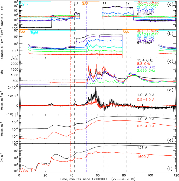
Figure 7. Time profiles of the M6.5 solar flare electromagnetic emissions on 2015 June 22. (a) Corrected RHESSI count rates in the six standard X-ray energy channels. The time intervals when the spacecraft was in the shadow of Earth (Night) and in the South Atlantic Anomaly (SAA) are shown with the cyan and orange horizontal thick lines, respectively. (b) Fermi/GBM count rates in the six similar X-ray energy bands. The Night and SAA time intervals for the Fermi spacecraft are also shown on the top with the same colors as in panel (a). (c) Flux density of solar microwave emission at four fixed frequencies detected by one of the Radio Solar Telescope Network (RSTN) observatories in Palehua. (d) Time derivative of the GOES/XRS 1.0–8.0 Å (black) and 0.5–1.0 Å (red) X-ray light curves, which are shown in panel (e) by the same colors. (f) The pre-flare background-subtracted light curves of the EUV and UV emissions in the SDO/AIA 131 and 1600 Å channels integrated over the flare region that is shown in Figure 8. The vertical dashed–dotted red and blue lines indicate the official flare start, at 17:39 UT, according to the GOES observations in the 1.0–8.0 Å channel and the beginning of the flare impulsive phase (at around 17:51:30 UT), respectively. The vertical black dashed and dotted lines show the beginning and end, respectively, of three time intervals (t0, t1, and t2) for which the images of the flare X-ray sources shown in Figure 8 are constructed.
Download figure:
Standard image High-resolution imageThe impulsive phase of the flare began at about 17:51:30 UT and was accompanied by the appearance of a sequence of bursts of nonthermal hard X-ray and microwave radiation associated with the appearance of populations of accelerated electrons in flare loops. Unfortunately, RHESSI was located within the South Atlantic Anomaly (SAA) in the time interval from 17:46 UT to 18:03 UT and missed the beginning of the impulsive phase (Figure 7(a)). However, hard X-ray emission from the flare during this time interval was detected by the Fermi Gamma-Ray Burst Monitor (GBM; Meegan et al. 2009, see Figure 7(b)). The time derivative of the soft X-ray emission measured by GOES/XRS roughly mimics the nonthermal flare emissions (microwaves and hard X-rays ≳50 keV), at least in the first half of the impulsive phase (the so-called Neupert effect; Neupert 1968; Dennis & Zarro 1993), and has a main peak around 17:58:36 UT (Figure 7(d)). At about the same time, a peak of UV radiation was observed in the SDO/AIA 1600 Å channel, emitted from the flare ribbons in the chromospheric feet of the flare loops. This peak roughly coincides with the peaks of hard X-ray and microwave radiation (Figures 7(b) and (c)), indicating that, at least at this time, accelerated electrons precipitating from coronal sources could efficiently heat the chromospheric plasma.
As an example, in Figure 8 we present images of flare sources of soft (≲25 keV) and hard (≳25 keV) X-ray emission for three time intervals: t0 (17:42:40–17:43:20 UT) at the beginning of the impulsive phase (panels (a)–(c)), t1 (18:04:00–18:07:00 UT) including several emission peaks in the impulsive phase (panels (d)–(f)), and t2 (18:21:40—18:25:28 UT) in the vicinity of the main peak of the flare soft X-ray emission (panels (g)–(i)). The start and end times of these intervals are shown in Figure 7 with the black vertical dashed and dotted lines, respectively. The duration of the selected intervals is long to provide a sufficient signal-to-noise ratio for constructing high-quality X-ray images. X-ray images were constructed using data from the RHESSI front detectors 3, 4, 5, 6, 7, and 8 using the Clean algorithm (Hurford et al. 2002). The images of X-ray sources are superimposed on SDO/AIA images in the 131 Å (panels (a), (d), and (g)) and 1600 Å (panels (b), (e), and (h)) channels (corresponding to plasma temperatures ∼10 and ∼0.1 MK, i.e., the energies of emitting ions ∼1 keV and ∼10 eV, respectively) and on the nearby 720 s HMI/SDO magnetograms of the line-of-sight magnetic field component (panels (c), (f), and (i)), which approximately equals the radial magnetic component, Br , because the flare region is located near the solar disk center. Images in the 131 Å channel predominantly show the flare loops filled with hot plasma heated to temperatures T ∼ 10 MK (∼1 keV), while images in the 1600 Å channel show the flare ribbons in the chromosphere and transition region (more details about the flare ribbons in this event were presented by Jing et al. 2016; Liu et al. 2018). All images show the position of the magnetic PIL on the photosphere (pink curves), as one of the traditional landmarks of the flare region. The impulsive phase of the flare (around t0) began in a system of highly sheared loops extended along the PIL (see also Wang et al. 2017; Kang et al. 2019). At this time, X-ray sources were co-located with these loops above the PIL. No hard X-ray sources with energies above around 50 keV were visible. The flare ribbons were very close to the PIL at that time. As the flare progressed (see Figures 8(d)–(f) and (g)–(i)), the ribbons grew larger and moved away from the PIL, and the flare loops became larger and taller, indicating an increase in the height of the primary energy release cite(s) in the corona with time. One can see the appearance of hard X-ray footpoints with energies ∼100 keV in t1 and t2, indicating the precipitation of accelerated electrons of corresponding energies into the feet of the flare loops in the chromosphere.

Figure 8. Images of the studied solar flare region for the three time intervals (a–c) t0, (d–f) t1, and (g–i) t2 indicated by the vertical dashed and dotted black lines in Figure 7. The background images in the left column show flare loops in the corona observed in the SDO/AIA 131 Å channel. The background images in the middle column show flare ribbons in the chromosphere and transition region observed in the SDO/AIA 1600 Å channel. The background images in the right column are the 720 s line-of-sight photospheric magnetograms made with the SDO/HMI instrument data. The color palette ranges from −2500 G (black) to +2500 G (white). The observational times are shown above the figures. Curves of different colors show isocontours at a level of 50% of the maximum brightness of X-ray sources in the 6–12 keV (orange), 12–25 keV (cyan), 25–50 keV (blue), and 50–100 (red) keV ranges, reconstructed in the time intervals t0, t1, and t2 from the RHESSI data using the Clean algorithm. The pink contours show the magnetic polarity inversion line (PIL) at the photosphere in the central part of the flare region. The Helioprojective-Cartesian coordinates are shown on the axes (e.g., Thompson 2006).
Download figure:
Standard image High-resolution imageHard X-ray and microwave emissions in the flare impulsive phase, near 18:05:32 UT (within t1), were investigated by Kuroda et al. (2018) using spatially and spectrally resolved observations by RHESSI and the Expanded Owens Valley Solar Array (EOVSA), respectively. Combining the NLFFF extrapolation and 3D modeling within the GX Simulator (e.g., Nita et al. 2015), at least two populations of accelerated electrons can be seen in the flare region. The first has a broken power-law spectrum (Ebreak ≈ 180–220 keV) and was trapped in the flare loops producing the high-frequency part of the microwave spectrum. The precipitating part of these electrons produced the observed hard X-ray footpoints. The second population of nonthermal electrons was trapped in a large volume (called the overarching loop) with relatively weak magnetic field above the main flare loops and was invisible in the hard X-ray range according to the RHESSI observations, while it was observed by its gyrosynchrotron radiation emitted mainly in the low-frequency microwave range. Overall, the results by Kuroda et al. (2018) showed good correspondence with the standard 3D eruptive flare model, where electrons are accelerated in the reconnection site(s) in the corona and trapped and precipitated in the complicated system of multiple underlying loops.
The interesting feature of X-ray and EUV/UV emission comparison (shown in Figure 8) is that the X-ray sources are more localized, i.e., the soft X-ray sources (≤25 keV) overlap only with a fraction of the flare coronal loops seen in the EUV range, and the hard X-ray sources (≥25 keV) occupy only a small fraction of the UV flare ribbons. It is unlikely that such localization of X-ray sources can be fully explained by the lower dynamic range and angular resolution of the RHESSI. One could assume that the most efficient acceleration of electrons occurs locally (i.e., in a small fraction of the flare arcade's loops), while less efficient energization (to the lower energies) of plasma happens in the much larger volume at a given time. In the substorm optical observations of emissions from the nonthermal electron (>1 keV) precipitations to the ionosphere also show stronger localization (less diffusive and more bursty structure) of such emission in comparison with diffusive emissions from <1 keV electron precipitations (see Figure 6). However, in the absence of collisional energy losses within the magnetotail, a difference between <1 keV and >1 keV emissions is mostly likely due to the difference of spatial scales of mechanisms responsible for general heating (<1 keV) and acceleration of nonthermal (>1 keV) populations. Although <1 keV and >1 keV electrons are produced as a result of adiabatic processes of magnetic field line shrinking in the post-reconnection magnetotail (Gabrielse et al. 2014; Birn et al. 2015), a seed population of <1 keV electrons is likely subthermal background plasma (electron temperature in the magnetotail is ∼0.1–0.5 keV (see Artemyev et al. 2011), and adiabatic heating in reconnection plasma flows can produce few keV electrons (see Runov et al. 2015, 2018)), whereas a seed population of >1 keV electrons is likely the population of electrons accelerated within the reconnection region (Imada et al. 2007, 2011; Asano et al. 2010; Egedal et al. 2012). Birn et al. (2017) showed that for flares a simple magnetic trap collapse (the analog of magnetic field line shrinking in the magnetotail) cannot produce nonthermal electron populations (often observed as a primary source responsible for hard X-ray emission; see, e.g., Oka et al. 2013), and additional scattering and acceleration mechanisms (e.g., direct acceleration by reconnection electric fields; see Gordovskyy et al. 2010) are needed. Thus, there is some analogy in the way thermal and nonthermal electron production occurs in the substorm magnetotail and in solar flares.
3.2.2. Dynamics of Magnetic Field and Current
Figure 9 shows spatial distributions of magnetic field components (and the absolute value of the full vector) and vertical current density at the photosphere in the active region around 3 minutes before flare onset at ∼17:36 UT. The vertical electric current density, jz , is calculated from Ampere's law, using the 720 s HMI/SDO vector magnetogram. The distribution of jz (shown in Figure 9(a)) can be compared with the current system formed at Earth's ionosphere and reconstructed from the ground-based magnetometer network (see Figure 4(a)). There are vertical currents of opposite polarities around the magnetic PIL, and those currents are probably at least partially closed by a return current system, not well seen in Figure 9(a) (see the discussion in Schmieder & Aulanier 2018). Due to the presence of strong magnetic shear (seen as the enhanced horizontal magnetic field component around the PIL in Figure 9(c); see also Wang et al. 2017; Wheatland et al. 2018; Kang et al. 2019), currents in the photosphere are not directly connected by cross-field currents (as opposed to the ionosphere; see Figure 4(a)), but rather connected by currents flowing almost along the PIL. Additional vertical currents formed during the solar flare (see below) should be closed at the top of the flare magnetic loops by currents composed of energetic particles accelerated at the energy release region. This magnetic field configuration differs from the substorm one, but there is a good analogy between physics of substorm and flare systems: both these systems connect cold collisional photospheric (ionospheric) plasma and hot collisionless plasma of the primary energy release cite(s).
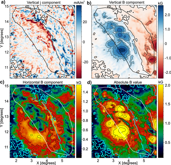
Figure 9. Maps showing the distribution of (a) vertical electric current density, (b) vertical magnetic field, (c) horizontal magnetic field, and (d) absolute magnetic field value at the photosphere deduced from the 720 s SDO/HMI vector magnetogram at around 17:36 UT, just before the official flare onset. The thin black (in panels (a) and (b)) and cyan (in panels (c) and (d)) curves show the magnetic PIL. The thick black (in panels (a) and (b)) and white (in panels (c) and (d)) closed contour indicates the outer boundary of the flare region around the PIL selected to calculate different magnetic field and electric current characteristics shown in Figure 10. The Stonyhurst heliographic coordinates are shown on the axes (e.g., Thompson 2006).
Download figure:
Standard image High-resolution imageFigures 10(a) and (b) compare the dynamics of the total absolute vertical current and current density (separately for the positive and negative directions) in the flare region (shown in Figure 9) and soft X-ray emission measured by GOES/XRS. Here the vertical current is calculated from Ampere's law using the sequence of 135 s HMI/SDO vector magnetograms. A method for calculating the vertical current and estimating measurement errors is presented in Sharykin et al. (2020). We considered only current values exceeding three standard deviations (>3σ) calculated for the background region on the Sun. There is a clear correlation between the dynamics of the total vertical current (both positive and negative) and soft X-rays emitted by plasma energized in the flare region. Thanks to the high time resolution of 135 s, one can even see the correspondence between individual spikes of X-ray emission and vertical current, in particular, during the precursors (∼17:20 UT and ∼17:40 UT), as well as toward the end of the flare at ∼21:10 UT and ∼22:30 UT. This figure shows an interesting analog to Figure 5: intervals of the strongest growth of the vertical current correlate with energetic electron precipitations to the ionosphere (as shown by the riometer measurements) and intensifications of hard X-ray and microwave emissions (corresponding to energetic electron precipitations to the flare loop footpoints; see, e.g., Krucker et al. 2008). Therefore, both systems demonstrate that the formation of the vertical currents is associated with the generation and precipitations of the energetic electrons. The time profile of the vertical current density correlates better with soft X-ray emission (i.e., follows the plasma heating), whereas Figure 5 shows the vertical current correlation with energetic (>30 keV) electron and ion fluxes. These are likely trapped fluxes, and their temporal variations well correlate with the plasma heating in the magnetotail (compare Figures 2, 5, and 6). Therefore, in both systems the vertical current dynamics are associated with the plasma heating (and formation of long-living trapped energetic fluxes in the magnetotail).
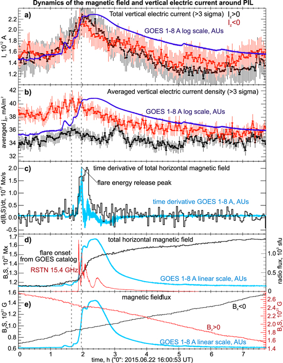
Figure 10. Temporal evolution of different characteristics of magnetic field and vertical electric current at the photosphere in the flare region (marked by the thick black or white contour in Figure 9). Absolute values of the total vertical current and current density are shown in panels (a) and (b), respectively (positive—black; negative—red). Estimated errors are shown with the vertical bars. The light curve of the solar soft X-ray emission detected by GOES/XRS in the 1–8 Å range is shown in the logarithmic scale (in arbitrary units) in dark blue. Time derivatives of the horizontal magnetic flux (black) and GOES 1–8 Å light curve (blue) are shown in panel (c). Absolute values of the total horizontal and vertical magnetic fluxes are shown in black in panel (d) and in black (for negative polarity) and red (for positive polarity) in panel (e), respectively. The light curve of the GOES 1–8 Å in the linear scale (in arbitrary units) is shown in blue in panels (d) and (e). The red curve in panel (d) shows the background-subtracted time profile of the solar radio flux density at 15.4 GHz detected by the RSTN/Palehua. The left and right vertical dashed lines show the official flare start at 17:39 UT and the maximum of the GOES 1–8 Å time derivative, respectively.
Download figure:
Standard image High-resolution imageWell-seen correlations of current intensities and energetic (>30 keV) particle/soft X-ray (≤25 keV) fluxes for the substorm and flare, respectively, may suggest that there is a certain similarity between these two systems. The inflow/outflow currents on the photosphere and ionosphere should be closed to currents of energetic particles around the energy release cite(s) at the top of the loop or in the near-Earth magnetotail. This region is filled by energetic particles drifting across magnetic field lines (or streaming along these lines in case of the strong magnetic field shear in the solar flare) and carrying intense currents. In the magnetotail filled by hot plasma (with the plasma β well exceeding 100) these currents are transverse to the magnetic field, whereas in the solar flares these currents would be field aligned or transverse (depending on the value of plasma β; see discussion in Gary 2001). The growth of these currents (and of field-aligned currents measured at the photosphere/ionosphere) should be associated with the increase of energetic particle fluxes due to injections from the reconnection region (i.e., from the primary energy release cite). Observations of an increase in vertical currents in the photosphere during several flares and a discussion of their association with reconnection in the corona can be found in, e.g., Janvier et al. (2014, 2016), Musset et al. (2015), Schmieder & Aulanier (2018), and Sharykin et al. (2020). This scenario is well consistent with in situ spacecraft observations in the magnetotail (see Figures 2–4 and Angelopoulos et al. 2008a, 2013; Sergeev et al. 2008). Thus, currents' dynamics reflect well the general plasma (heating) energization during the onset of energy release. However, the subsequent slow decay of the current density and energetic particle fluxes may be quite different for substorms and flares. During the quite long (∼40 minutes) periods of currents/flux dynamics in the magnetotail, there are only two energy release events associated with strong electron precipitations (see Figure 5), whereas most of the time strong fluxes of energetic particles are trapped within the magnetotail current sheet, and drifts of these particles generate currents connected to the ionosphere through the field-aligned inflow/outflow currents shown in Figure 4. The loss-cone size in the solar flare magnetic loop is much larger than in the magnetotail (typical loss-cone size in the magnetotail magnetic field is  ; see Figure 3(d) in Zhang et al. 2015; in comparison with tens of degrees in solar flare magnetic loops; see Aschwanden et al. 1996a, 1996b), and most of the energetic particles are expected to precipitate quickly after energy release. Thus, there are two possible scenarios that can explain long-term evolution (decay) of currents and soft X-ray emission in Figure 10. First, there can be continuous series of energy releases that accelerate new particles and guarantee that the level of energetic particles would be sufficiently high during a long decay phase (e.g., Dere & Cook 1979; Zimovets & Struminsky 2012; Qiu & Longcope 2016; Yu et al. 2020). Second, there can be strong magnetic turbulence trapping initially energized particles around the top of the flare loops (see discussion in Karlický & Kosugi 2004; Grady & Neukirch 2009). The second scenario, in which fewer energy release bursts occur and the lifetime of energetic particle fluxes and currents is longer, appears to be much closer to what occurs in magnetospheric substorms.
Figure 10(d) compares dynamics of the horizontal magnetic flux (i.e., the horizontal magnetic field component multiplied by pixel area and integrated over the flare region containing the inflow/outflow or negative/positive currents shown in Figure 9(a); see details of method in Sharykin et al. 2020) and soft X-ray emission flux in the GOES/XRS 1–8 Å channel. The increase of the horizontal magnetic flux correlates well with soft X-ray flux produced by hot plasma in the flare region. This correlation is also clearly visible in Figure 10(c), which shows the time derivatives of the horizontal magnetic flux and soft X-ray flux. At the same time, it can be noted that the flux of the vertical magnetic field changes relatively smoothly before, during, and after the flare and does not show a jump during the growth of X-ray flux (Figure 10(e)). A step-like increase in the horizontal component of the magnetic field in the flare region near the PIL is also detected in other flares (e.g., Petrie 2013; Sun et al. 2017; Sharykin et al. 2020). There is a direct analogy with the magnetic flux increase in the near-Earth region shown in Figure 5. For Earth's magnetotail such a magnetic field increase is due to magnetic flux transport from the energy release region to the near-Earth side, where the strong dipole field breaks the plasma flow (for details of such flux increase correlation with the energetic electron precipitations, see, e.g., Gabrielse et al. 2019). Around the flow-breaking region magnetic flux accumulates, leading to the formation of the magnetic pileup region. This region expands toward the magnetotail, which can switch off the magnetic reconnection (Baumjohann 2002). Strong magnetic field within this region traps energetic particles (e.g., Turner et al. 2016; Gabrielse et al. 2017, and references therein). Oscillations of the outer boundary (edge) of this region are generally seen (e.g., Panov et al. 2010) as a quasi-periodic increase of the equatorial Bz (corresponding to Bh for the solar flare). MMS observations of Bz oscillations (see Figure 2) may be interpreted within this context, although MMS location in the middle tail and quite small Bz < 10 nT suggest that these oscillations also can be driven by plasma vortexes often observed around fast plasma flows (e.g., Birn et al. 2011; Vörös 2011).
Does the same mechanism of energetic particle trapping work for solar flares, and can this mechanism substitute/supplement trapping by magnetic field turbulence? Although the horizontal magnetic flux increase shown in Figures 10(c) and (d) indicates such similarity, additional confirmation is needed. A possible data set of observations that would show energetic particle trapping due to magnetic field increase at the top of the loops is the spatially localized and spectrally resolved gyrosynchrotron emission that is presumably generated within the regions of enhanced magnetic field. In some flares, there is indeed increased microwave emission at the tops (or above them) of the flare loops, indicating efficient electron trapping in these regions (e.g., Melnikov et al. 2002; Minoshima et al. 2008; Huang & Nakajima 2009; Reznikova et al. 2009). However, these studies did not establish temporal changes in the magnetic field at the loop tops during the flares studied. The accumulation of energetic electrons at the loop tops was interpreted as trapping due to the specific anisotropic pitch-angle distributions of the injected accelerated electrons. In some works, the possible influence of turbulence on the efficiency of trapping of energetic electrons in flare loops was discussed (e.g., Charikov & Shabalin 2015; Filatov & Melnikov 2020). Most recently, Fleishman et al. (2020), based on the analysis of spatially and spectrally resolved microwave observations with EOVSA, showed a simultaneous decrease in the magnetic field (and magnetic energy density) with an increase in the energy density of nonthermal electrons in the region above the flare loops in the solar flare on 2017 September 10. This result was interpreted by transformation of magnetic energy into kinetic energy of accelerated electrons due to magnetic reconnection within the standard eruptive flare model. However, we are not aware of studies in which a simultaneous increase in the longitudinal (Bh ) component of the magnetic field at the top of the flare loops and an increase in the density of nonthermal electrons are demonstrated.
4. Discussion and Conclusions
This section presents the substorm observational data set with an eye to solar flare observations, discussing in turn the formation of the substorm/flare current systems, energetic particle fluxes, and thermal versus nonthermal electron populations. We conclude with a table summarizing data set comparisons for substorms and flares.
4.1. Formation of Substorm/Flare Current System
Both magnetotail substorm and solar flare demonstrate formation of a system of intense field-aligned currents that connects a region of hot plasma (energy release region) and a region of dense (conductive) cold plasma (ionosphere or photosphere). In Earth's magnetotail such a system originates from the dynamics of plasma flows generated at the energy release region, breaking in the near-Earth strong dipole field region (see simulations by Birn et al. 2011; Birn & Hesse 2013; El-Alaoui et al. 2013). The main equation describing field-aligned current closure to the cross-field currents within the flow-breaking region is the divergence-free equation of currents (Vasyliunas 1970), i.e., the basic physics of such a field-aligned current system is well described within MHD models and should be well reproduced in global MHD simulations of solar flares. Assuming this similarity between these systems, we can make several comments about the kinetics of field-aligned currents. From the magnetotail observations we know that, being generated as a global MHD system of field-aligned currents, this system quickly involves ion-scale and electron-scale kinetics (see reviews by Lysak 1990; Stasiewicz et al. 2000). Most relevant to solar flares is the filamentation of field-aligned currents due to transformation of Alfvén waves (carrying such currents) to kinetic or inertial Alfvén waves (Lysak 2004; Lysak et al. 2013; Chaston et al. 2014). Such transformations are quite important, as they open the door to collisionless dissipation of currents by thermal (<1 keV) electrons accelerated by field-aligned electric fields of kinetic/inertial Alfvén waves (see discussion of these processes in application to the solar corona in, e.g., Fletcher & Hudson 2008; Haerendel 2012; Artemyev et al. 2016). Therefore, some elements of kinetic physics from substorm observations (e.g., efficiency of electron acceleration/field-aligned current damping; see Damiano et al. 2016; Sharma Pyakurel et al. 2018) may be implemented into solar flare models. Moreover, ground-based observations of substorms show a direct relation between enhanced horizontal currents and electric fields around field-aligned currents (Opgenoorth et al. 1983). Such observations may be useful for investigation and simulations of electric fields at photospheric levels (see discussion of this analogy in Kropotkin 2011; Krasnoselskikh et al. 2012).
For the interpretation of changes in the magnetic fields and vertical currents in the investigated flare of 2015 June 22, Wheatland et al. (2018) propose a simplified analytical model based on the response of the photosphere to a large-amplitude Alfvén wave propagating downward from the energy release site in the corona. The wave brings magnetic and velocity shears into the photosphere, which can qualitatively explain the observed changes. Wheatland et al. (2018) also raised the issue that electrons can be accelerated in the field-aligned electric field at the front of this large-scale Alfvén wave. To fulfill the condition that this field-aligned electric field exceeds the Dreicer field (when electrons can be effectively accelerated in the runaway mode), the front width should be rather narrow, ≃10 m. However, Wheatland et al. (2018) mentioned that in the presence of an anomalous resistivity due to turbulence or microscale structures, the required front thickness could be much larger. Although large-scale Alfvén wave transformation into kinetic/inertial Alfvén waves was not considered by Wheatland et al. (2018), the general issue of energy cascade from the large to small scales in Alfvén wave turbulence is quite similar for both magnetotail and solar corona systems.
4.2. Energetic Particle Fluxes and Their Correlation with Currents
Both substorms and flares demonstrate a correlation of energetic (>30 keV for the magnetotail) particle fluxes/X-ray emission (tens of keV for solar flares) with the dynamics of electric currents. This correlation is well explained and modeled for the magnetotail, where ionospheric currents are closed through the magnetotail currents generated by plasma flow shear and energetic particle drifts associated with the pressure gradients (Kepko et al. 2014; Ganushkina et al. 2015). However, this explanation is based on the concept that energetic particles are trapped in the near-Earth region for a long time, and their precipitations into the narrow loss cone (couple degrees) are driven by weak pitch-angle diffusion due to curvature scattering (working mostly for energetic ions; see Sergeev et al. 2012, 2015; but contributing to electron losses as well; see Artemyev et al. 2013; Eshetu et al. 2018) and wave turbulence (working mostly for energetic electrons; see Nishimura et al. 2010, 2020; Ni et al. 2016).
This is one of the important differences between substorms and solar flares: the loss cone in the magnetotail is quite small (≤2°; see, e.g., Figure 3(d) in Zhang et al. 2015), and accelerated particles can be trapped on closed magnetic field lines for a long time (e.g., in our event MMS observed increased fluxes for 40 minutes after the primary energy release), whereas the loss cone in solar flare configurations is much larger (Aschwanden et al. 1996a, 1996b). Therefore, additional trapping mechanisms are required to provide stable trapping of accelerated particles at the top of the flare loop and prevent their quick precipitation (see discussion in Eradat Oskoui et al. 2014). Two perspective mechanisms providing such trapping are pitch-angle scattering away from the loss cone (e.g., Kontar et al. 2014; Charikov & Shabalin 2015) by plasma turbulence (see discussion in Hannah & Kontar 2011; Fleishman et al. 2018, 2020) and pitch-angle increase by magnetic field line shrinking (magnetic trap collapse; see, e.g., Karlický & Bárta 2006). Alternatively, energetic particle populations can be continuously supplemented by series of transient energy releases. The first scenario (trapping by scattering and magnetic field line shrinking) would resemble a weak isolated magnetotail substorm (shown in this study), whereas the second scenario is an analog of multiple substorms occurring within a strong geomagnetic storm (see, e.g., Gabrielse et al. 2017; Angelopoulos et al. 2020).
If we assume that the correlation of energetic fluxes and currents has similar origins in substorms and flares, we can speculate on the importance of elements of substorm physics for solar flares. First, strong drifts (different for ions and electrons) of energetic particles trapped in the near-Earth magnetotail result in electric polarization of this region. Such electric fields are projected along magnetic field lines to the ionosphere and are observed as ionospheric plasma drifts (Sergeev et al. 2004). Similar observations of photosphere cross-field plasma motions (see discussion in, e.g., Krasnoselskikh et al. 2010) may be interpreted in terms of electric fields dynamics in analogy to the ionosphere–magnetosphere coupling investigations. Second, energetic particle populations in the near-Earth magnetotail create a strong pressure gradient unstable to various plasma drift modes. Plasma and field perturbations by unstable waves are well seen in in situ measurements (e.g., Panov et al. 2012, 2013), numerical simulations (e.g., Pritchett & Coroniti 2010; Pritchett et al. 2014; Sorathia et al. 2020), and ground-based optical observations (e.g., Nishimura et al. 2016). Similar waves are expected to develop at the apex of flare loops, where the breaking of plasma flows from the energy release region occurs. The properties of such waves, generated by pressure gradients of energetic particles, may be used for estimates of characteristics of energetic particle populations. Indeed, oscillations and/or quasi-periodic pulsations (QPPs) are observed at least in some flares in the vicinity of the loop tops, where nonthermal electrons are present (e.g., Jakimiec & Tomczak 2010; Yuan et al. 2019; Reeves et al. 2020). The nature of these oscillations is not yet clear (see the review by Zimovets et al. 2021). According to the MHD model developed by Takasao & Shibata (2016), these oscillations can result from the formation of a magnetic tuning fork structure at the tops of reconnected loops due to their interaction with accelerated plasma flows falling from the reconnection region from above. However, other mechanisms for these oscillations cannot be ruled out so far, and research should be continued, in particular, taking into account the aforementioned physical processes established for magnetospheric substorms.
4.3. Thermal versus Nonthermal Electron Populations
Both substorms and flares demonstrate differences in spatial localizations of emissions associated with the precipitation of energetic (several tens of keV and more) and hot (≤1 keV) electrons. UV (and optical) emission from the flare ribbons shows heating of plasma in the feet of flare loops connected to the energy release cite(s) in the corona (see Figure 8). Similar heating is observed in the magnetotail current sheet during the substorm and detected both by in situ measurements (the increase of electron temperature and high-energy flux magnitude; see Figures 3, 6(c), (d)) and optical observations of electron precipitations into the ionosphere (see Figures 5(e), 6(a), (b)). Such optical observations from the ground-based all-sky cameras and measurements of riometer stations show that emissions due to >1 keV electron precipitations to the ionosphere are much more spatially localized and temporally transient than emissions due to <1 keV precipitations, whereas riometer measurements (tens of keV electron precipitations) show even stronger temporal localization. Similarly, hard X-ray and microwave emissions are more bursty than soft X-ray and UV/EUV emissions (see Figure 7), and the hard X-ray sources are usually much more localized than the extended flare ribbons observed in UV and optical (e.g., Hα) ranges and soft X-ray and EUV flare loops rooted in these ribbons (see Figure 8 and also, e.g., Temmer et al. 2007; Fletcher et al. 2011). It can be assumed that at any time interval during the flare, electrons are injected/accelerated most efficiently only in some specific field lines (in some loops), and on other field lines (in other loops of the flare magnetic arcade) electrons are much less energized. A real flare has an essentially 3D configuration without translational symmetry along the PIL, i.e., it is important to take into account the development of reconnection and particle energization processes not only at difference heights but also at different locations along the PIL (e.g., Grigis & Benz 2005; Qiu & Longcope 2016; Janvier 2017).
In contrast to collisional heating within chromosphere, the main plasma heating mechanism in the magnetosphere is the collisionless adiabatic heating of electrons and ions trapped within shrinking magnetic flux tubes (Birn et al. 2015; Ukhorskiy et al. 2018; Eshetu et al. 2019). This heating mechanism resembles the magnetic trap collapse described in application to solar flares by Karlický & Kosugi (2004), Bogachev & Somov (2005), Birn et al. (2007), and Borissov et al. (2016). Such heating at the top of the coronal loop can be quite effective in both 2D and 3D magnetic trap configurations (see estimates in Grady & Neukirch 2009), but the main plasma heating within the loops (responsible for the UV and optical emissions in the loops' feet) is most likely due to collisional plasma heating by energetic precipitating particles (although thermal conduction variations also may contribute to plasma temperature increase in the loop; see Rust & Somov 1984; Reep et al. 2016; Ashfield & Longcope 2021).
For magnetospheric substorms, the localization of energetic particles as seen in the ground-based measurements can be explained by the spatial localization of the inferred source of those particles. Simulations (e.g., Birn et al. 2015; Gabrielse et al. 2016, 2017) and observations (e.g., Runov et al. 2015) show that the main energization occurs within fast plasma flows (especially at the flow front called the dipolarization front; see Nakamura et al. 2004; Sergeev et al. 2009; Runov et al. 2011). These flows are responsible for magnetic field compression and field line shrinking that adiabatically energize both thermal (≤ a few keV) and energetic (>30 keV) electron populations, although how much of the energization process is adiabatic depends on the initial electron energy. The energization of the pre-existing cold (<1 keV) population should follow this scenario and should result in heating from 0.1 to a few keV while traveling along the outflow (e.g., Runov et al. 2014; Gabrielse et al. 2017). Such a heated population is thus distributed over a wide range of space between the flow-braking region and the reconnection X-line, leading to the diffuse signature in the ground-based measurements of electron precipitations within this energy range. In contrast, particles with much higher energies (∼10 keV) can be produced during an energy release by magnetic reconnection and associated electric field bursts (see Egedal et al. 2012; Torbert et al. 2018; Angelopoulos et al. 2020). While these particles could be further energized to tens and even hundreds of keV in the magnetotail (Fu et al. 2013; Runov et al. 2013), they are basically produced near the reconnection X-line, which is spatially localized in the outflow direction (Cohen et al. 2021; Turner et al. 2021). The localized acceleration region (i.e., the X-line and its vicinity) can be magnetically connected to the ionosphere, and the energized particles can directly precipitate without being transported to the flow-braking region, leading to the localized signature in the ground-based measurements.
We may adopt a similar logic for flares, where the most intense acceleration would be localized around the energy release region (e.g., Aschwanden 2002; Zharkova et al. 2011, and references therein), whereas the energization of the larger plasma populations can be associated with the adiabatic heating driven by the magnetic field reconfiguration (see discussion in Birn et al. 2017). Therefore, in both systems (magnetotail and solar flares) direct acceleration within the reconnection region is likely limited to a relatively small charged particle population (e.g., Imada et al. 2011; Cohen et al. 2021; Turner et al. 2021), because of the transient nature of the reconnection (a short lifetime), a spatial localization of the reconnection region, and instability of particle motion there (see discussion in Bulanov & Sasorov 1976; Zelenyi et al. 1990; Litvinenko 1996, 2003; Vekstein & Browning 1997; Browning & Vekstein 2001; Hannah & Fletcher 2006; Artemyev et al. 2014). However, reconnection releases a significant portion of energy in the form of plasma flows and intense electromagnetic waves that collapse the magnetic field and effectively accelerate large plasma volumes in the magnetotail (e.g., Imada et al. 2007; Birn et al. 2014; Runov et al. 2015; Sorathia et al. 2018) and solar flares (e.g., Karlický & Bárta 2006; Birn et al. 2007, 2017; Eradat Oskoui & Neukirch 2014; Borissov et al. 2016).
4.4. On Kinetic Scales of Currents
The comparative analysis in this study focused on mesoscale processes, such as plasma flows and current systems connecting the energy release region and cold dense plasma volumes. At these scales, basic processes of the solar flare and magnetospheric substorm can be compared and analogies between these processes can be drawn. In situ spacecraft observations, however, provide detailed information on processes with smaller spatial and temporal scales contributing to the energy release and transport during magnetospheric substorms. The most investigated ion kinetic (with spatial scales comparable to ion thermal gyroradius) processes are formation of parallel electric fields in Alfvén wave turbulence (e.g., Rankin et al. 1999; Lysak et al. 2013) and thin intense current sheets (see, e.g., Artemyev et al. 2021; Runov et al. 2021; Sitnov et al. 2021, sand references therein) that play a dominant role in dissipating magnetic energy during substorm reconnection (e.g., Nakamura et al. 2006; Eastwood et al. 2013; Sitnov et al. 2018). Investigations on electron kinetics (sub-ion spatial scales) have started since the MMS mission, which provides plasma measurements on sub-ion temporal scales (Burch et al. 2016a). The most relevant discovery from MMS is the electron-scale reconnection, which is characterized by all signatures of magnetic field line reconnection and magnetic energy transformation to plasma heating and acceleration but does not include any ion dynamics (Phan et al. 2018). These electron-scale reconnecting current sheets can survive long enough to provide electron acceleration in turbulent (Stawarz et al. 2019) and laminar (Hubbert et al. 2021) plasmas. Although plasma dynamics on such scales are not measurable in solar flares, the well-documented magnetospheric observations may provide some basis for including these kinetic processes in the large-scale MHD simulations of solar flare dynamics. The flare–substorm analogies established at mesoscale processes suggest that magnetospheric observations may help in further incorporating plasma kinetics into such simulations.
4.5. Conclusions
In this study we compare several data sets available for solar flares and for magnetospheric substorms. Similarities of observations in terms of measured quantities or energy range of particles, illustrated via the comparative analysis of one typical substorm and one eruptive flare, are summarized in schematic Figure 11 and in Table 1. The main similarity discussed in this study is the common relation of current and energetic flux dynamics: rapid increase of inflow/outflow currents on the photosphere and ionosphere well correlates with energetic electron generation and precipitations (as shown by hard X-ray emissions and riometer signals), whereas long-term decay of currents correlates with dynamics of thermal (hot) electron fluxes within flare loops and near-Earth magnetotail (as shown by soft X-ray emissions and in situ plasma measurements in the magnetotail). Optical observations from the all-sky camera and X-ray (together with UV/EUV) emission for separated energies demonstrate the similar effect of more spatially localized precipitations from higher-energy electrons.

Figure 11. Schematic view of main similarities of substorms and flares discussed in Table 1. The bottom panel shows temporal profiles of currents, precipitations of energetic electrons (as seen by riometer and hard X-ray emission), and plasma heating (as seen by optical/in situ observations in the magnetosphere and by soft X-ray/EUV emissions in flares).
Download figure:
Standard image High-resolution image
Table 1. Data Set Comparison for Solar Flares and Magnetosphere Substorms
| Solar Flare | Magnetosphere Substorm | Comments |
|---|---|---|
| Photosphere magnetic field and reconstructed vertical currents | Ground-based field and reconstructed currents | Similar dynamics along the substorm/flare and similar closure to the energetic particle currents around energy release region |
| Hard X-ray microwave emissions from the flare loop footpoints | Riometer signals | Direct indication of >30–100 keV electron precipitations to the chromosphere/ionosphere from the energy release region |
| Hard X-ray and microwave emissions from the heated flare loops in the corona | In situ measurements of energetic fluxes | Similar correlation to current enhancements and direct relation to plasma energization by energy release |
| Soft X-ray, EUV, and thermal microwave emissions from the heated flare loops in the corona, and UV and optical emissions from the flare ribbons | Optical measurements of energetic electron precipitations | Similar emission generation mechanisms from hot and energetic electrons precipitating to the chromosphere/ionosphere |
Download table as: ASCIITypeset image
Used MMS, THEMIS, and ERG data can be downloaded from http://lasp. colorado.edu/mms/sdc, http://themis.ssl.berkeley.edu. Science data of the ERG (Arase) satellite were obtained from the ERG Science Center operated by ISAS/JAXA and ISEE/Nagoya University (https://ergsc.isee.nagoya-u.ac.jp/index.shtml.en; Miyoshi et al. 2018a).
NRCan riometer data used in this study may be obtained at https://doi.org/10.7910/DVN/CHD02S or by request from Robyn Fiori (Robyn.Fiori@canada.ca). Operational support for NORSTAR is provided by the Canadian Space Agency through the GO Canada program. NORSTAR data were made available directly from the University of Calgary and may be freely obtained from the Canadian Space Science Data Portal (http://www.cssdp.ca).
Data analysis was done using SPEDAS V3.1; see Angelopoulos et al. (2019). We are grateful to the teams of SDO/HMI, SDO/AIA, RHESSI, GOES/XRS, Fermi/GBM, and RSTN for the observational data provided.
The work is supported by the Russian Science Foundation grant No. 17-72-20134 (I.Z., I.S.; Section 3.2), NASA contract NAS502099 (A.A., A.R., V.A., X.Z.), NASA DRIVE SCIENCE CENTER HERMES grant No. 80NSSC20K0604 (A.A., A.R., Y.N., C.D., M.V., O.P.), NASA grants 80NSSC18K0657 and 80NSSC20K0725, NSF grant AGS-1907698, and AFOSR grant FA9559-16-1-0364 (Y.N.). This is Natural Resources Canada's publication 20210341 (R.F.). Part of this work (K.K.) was supported by the Ministry of Education, Culture, Sports, Science and Technology, Japan Society for the Promotion of Science (JSPS), Grant-in-Aid for Scientific Research (B) (19H01949, 20H01957).
The all-sky imager at the South Pole is supported by NSF ANT-1643700 and the Japanese Antarctic Research Expedition program.