


Abstract
Measurements of cosmic flows enable us to test whether cosmological models can accurately describe the evolution of the density field in the nearby universe. In this paper, we measure the low-order kinematic moments of the cosmic flow field, namely bulk flow and shear moments, using the Cosmicflows-4 Tully−Fisher catalog (CF4TF). To make accurate cosmological inferences with the CF4TF sample, it is important to make realistic mock catalogs. We present the mock sampling algorithm of CF4TF. These mocks can accurately realize the survey geometry and luminosity selection function, enabling researchers to explore how these systematics affect the measurements. These mocks can also be further used to estimate the covariance matrix and errors of the power spectrum and two-point correlation function in future work. In this paper, we use the mocks to test the cosmic flow estimator and find that the measurements are unbiased. The measured bulk flow in the local universe is 376 ± 23 (error) ± 183 (cosmic variance) km s−1 at depth dMLE = 35 Mpc h−1, to the Galactic direction of (l, b) = (298° ± 3°, −6° ± 3°). Both the measured bulk and shear moments are consistent with the concordance Λ Cold Dark Matter cosmological model predictions.
1. Introduction
Observations of galaxies indicate that there are fluctuations in the density field of local universe (Jarrett 2004 and references therein). The gravitational effects of the density perturbations exert additional velocity components to the galaxies' Hubble recessional velocities, called "peculiar velocities." These peculiar velocities are good probes of the density field, enabling us to constrain cosmological parameters and test cosmological models.
Due to the peculiar motions of galaxies, the apparent (or inferred) distance of a galaxy, dz is different from its true comoving distance, dh . This difference is measurable and quantified by the "logarithmic distance ratio" for that galaxy, defined as

The η of late-type galaxies can be measured from the Tully−Fisher relation (Tully & Fisher 1977; Strauss & Willick 1995; Masters et al. 2008; Hong et al. 2014), while for early-type galaxies, η can be measured from the Fundamental Plane (Djorgovski & Davis 1987; Dressler et al. 1987; Strauss & Willick 1995; Magoulas et al. 2012; Springob et al. 2014; Said et al. 2020). The peculiar velocity of a galaxy can be estimated from its log-distance ratio using velocity estimators (Davis & Scrimgeour 2014; Watkins & Feldman 2015; Adams & Blake 2017).
The cosmic flow field in the local universe arises from the peculiar velocities of galaxies. Measuring the low-order kinematic moments of the cosmic flow field, i.e., bulk flow and shear moments, from peculiar velocity surveys and comparing them to the Λ Cold Dark Matter theory predictions enables us to test whether the theory accurately describes the motion of galaxies on large scales. In previous work, the bulk and shear moments are commonly measured using two different methods: maximum likelihood estimation (MLE, Kaiser 1988) and minimum variance estimation (Watkins et al. 2009; Feldman et al. 2010). The measurements generally agree so far with the Λ Cold Dark Matter model (ΛCDM) prediction (Kaiser 1988; Staveley-Smith & Davies 1989; Jaffe & Kaiser 1995; Nusser & Davis 1995; Parnovsky et al. 2001; Nusser & Davis 2011; Turnbull et al. 2012; Ma & Scott 2013; Hong et al. 2014; Ma & Pan 2014; Scrimgeour et al. 2016; Qin et al. 2018, 2019b; Boruah et al. 2020; Qin 2021; Stahl et al. 2021).
In this paper we will measure the bulk flow and shear moments using the peculiar velocity catalog, Cosmicflows-4 Tully−Fisher catalog (CF4TF, Kourkchi et al. 2020b), and compare the measurements to the ΛCDM predictions to test the model. CF4TF is the currently largest full-sky catalog of Tully−Fisher galaxies, enabling us to more accurately measure the bulk and shear moments; the measurements are less affected by the an-isotropic sky coverage, comparing to previous work.
In addition, as CF4TF is one of the key components of the future full Cosmicflows-4 catalog, we present the mock sampling algorithm for CF4TF in this paper. Combining these CF4TF mocks with the 6dFGSv mocks (Qin et al. 2018, 2019a), we can obtain mock catalogs for the two largest subsets of the final full Cosmicflows-4 catalog. Our mocks can model the luminosity selection and survey geometry of the real surveys, enabling researchers to explore how these systematics affect the measurements (Qin et al. 2018, 2019b). In future work, these mocks can be used to study the power spectrum and two-point correlation of velocities of the Cosmicflows-4 catalog. They are the key to estimate the covariance matrix and errors of these measurements. They can also be used to test the methods of these measurements to identify any possible biases. The mock catalogs underlying this article will be shared upon a reasonable request to the corresponding author. In this paper, these mocks are used to test the cosmic flow (bulk and shear moments) estimator to explore how well the estimator recovers the true moments.
The paper is structured as follows. In Section 2, we introduce the CF4TF data. In Section 3, we introduce the L-PICOLA simulation (Howlett et al. 2015a, 2015b) and present the mock sampling algorithm. In Section 4, we introduce the cosmic flow estimator and test the estimator using mocks. We present the final results and discussion in Section 5. A conclusion is presented in Section 6.
We adopt a spatially flat ΛCDM cosmology as the fiducial model. The cosmological parameters are: Ωm = 0.3121, ΩΛ = 0.6825, and H0 = 100 h km s−1 Mpc−1 with h = 0.6751.
2. Data
The CF4TF (Kourkchi et al. 2020b) is a full-sky catalog of 9790 galaxies. The sky coverage of the CF4TF galaxies in Galactic coordinates is shown in Figure 1. The redshift of the CF4TF galaxies reaches 20,000 km s−1; the redshift distribution is shown in Figure 2. The distances of galaxies are measured using the Tully−Fisher relation (Tully & Fisher 1977; Kourkchi et al. 2020b), which is a linear relation between the H i rotation widths and photometric magnitudes.

Figure 1. The sky coverage of the CF4TF galaxies in Galactic coordinates. The colors of the dots represent the redshift of the galaxies according to the color bar.
Download figure:
Standard image High-resolution image
Figure 2. The redshift distribution of the CF4TF galaxies.
Download figure:
Standard image High-resolution imageThe H i data are taken from the following four catalogs. The primary catalog is the All Digital H i catalog (ADHI, Courtois et al. 2009); the galaxies with H i line width uncertainties ≤20 km s−1 are selected. In the ADHI, the galaxies below decl. δ = −45° are observed by the Parkes Telescope (Courtois et al. 2011); the number density of galaxies is lower in this region. Most of the remainder are from the Arecibo Legacy Fast ALFA Survey (ALFALFA, Haynes et al. 2018, 2011), mainly distributed in the decl. range [0°, 38°], and the galaxies with an H i spectrum signal-to-noise ratio S/N > 10 are selected. The rest are from the Springob/Cornell catalog (Springob et al. 2005) and the Pre-Digital H i catalog (Fisher & Tully 1981; Huchtmeier & Richter 1989).
The u-, g-, r-, i-, and z-band photometry is taken from the Sloan Digital Sky Survey (SDSS) Data Release 12 (DR12, York et al. 2000). The w1 and w2 band data are taken from the Wide-field Infrared Survey Explorer (WISE, Wright et al. 2010). The i-band absolute magnitude cut Mi ≤ −17 Mag is applied to the data (Kourkchi et al. 2020b, 2020a).
3. Mocks
3.1. L-PICOLA Simulation
Producing realistic mock surveys that model nonlinear gravitational interactions requires N-body simulations. However, such full N-body simulations, which model the gravitational forces and motions down to a fine resolution, can require an extensive HPC infrastructure and a large amount of CPU time. To make a large ensemble of mock surveys quickly and efficiently, we use the COmoving Lagrangian Acceleration (COLA) approach (Tassev et al. 2013) implemented in the l-picola code (Howlett et al. 2015a, 2015b).
We use l-picola to generate 250 dark matter simulations. Though approximate, this method and code have been demonstrated to reproduce the clustering of dark matter particles and halos well on all scales of interest for galaxy and peculiar velocity clustering (Howlett et al. 2015a, 2015b; Blot et al. 2019), at a ≳95% accuracy for both the power spectrum and bispectrum at k = 0.3h Mpc−1. Halos are identified in these simulations using the 3D friends-of-friends algorithm in the VELOCIraptor code (Elahi 2009). This code has also been demonstrated to recover realistic halos, subhalos, and halo merger trees (although we only use the first of these here), in agreement with a variety of other halo finders (Onions et al. 2012; Knebe et al. 2013).
The fiducial cosmology is given by Ωm = 0.3121, Ωb =0.0488, σ8 = 0.815, and h = 0.6751. The redshift of the simulations is at z = 0. The box size is 1800 Mpc h−1. The number of particles in each simulation is 25603. The minimum halo mass is ∼5 × 10¹¹ M☉ h−1 (20 particles per halo).
3.2. Mock Sampling Algorithm for CF4TF
We have 250 simulation boxes in total; each simulation provides us with the masses mhl of halos and the Cartesian positions [x, y, z] and velocities [vx , vy , vz ] of halos. We divide each simulation box into eight identically sized cubes. In each cube, the observer is placed at a galaxy close to the center of that cube. Therefore, we have generated 2000 mock CF4TF catalogs in total.
The halos in the simulations are parent halos; it is required to generate subhalos and galaxies from these parent halos. The starting point is the halo concentration, defined as

which characterizes the mass distribution in a halo. The term rv is the virial radius of a halo, rs is the break radius between an inner and outer density profile in a halo, and cv is computed purely as a function of parent halo mass mv using the fitted relationship from Prada et al. (2012), calibrated on high-resolution N-body simulations. The virial radius is also computed using the parent halo mass and assuming the halo is both spherical and has a density 200× the critical density of the universe. Given cv and rv , one can generate the subhalos and galaxies using the Navarro–Frenk–White (NFW) profile (Navarro et al. 1997).
The subhalo generation algorithm is based on Vale & Ostriker (2004), Conroy et al. (2006), Howlett et al. (2015c, 2017) and Qin et al. (2019a) and is detailed below. First, we assume a power-law distribution for the mass ratio between a subhalo and its parent halo. From this power-law distribution, we can compute the expected number of subhalos as (Springel et al. 2008; Giocoli et al. 2008; Elahi et al. 2018)

where fM is the mass ratio between the subhalo and its parent. Ratio fmin is the minimum mass ratio we consider, which we set, based on the minimum halo mass of the simulation (see Section 3.1), to 20 times the dark matter particle mass divided by the parent halo mass (i.e., a fixed minimum mass, such that the minimum mass ratio varies based on the parent halo). The free parameters A and αh will be fitted by matching the density power spectrum of mocks to real data.
To add realism to the sampling process, the actual number of subhalos in each parent halo Nsub is generated assuming a Poisson distribution with mean λPoi. The mass ratios of the Nsub subhalos are generated by drawing uniform random numbers in the interval [0, 1], and inverting the quantile distribution for Equation (3). This results in mass ratios in the interval . The subhalo masses are then obtained by multiplying the set of fM by the mass of the parent halo. As the largest value of fM generated for the Nsub subhalos is 1, the masses of the subhalos will not be larger than their parent halos.
![$[{f}_{\min },\,1]$](https://content.cld.iop.org/journals/0004-637X/922/1/59/revision1/apjac249dieqn1.gif)
The positions of subhalos are generated from the NFW profile following the arguments in Robotham & Howlett (2018), and rely on the concentration and virial radius for each parent halo computed as described previously . We generate Nsub random numbers in the interval R ∈ [0, 1], then calculate the position parameter (Robotham & Howlett 2018)

and the radius

which gives the radial position of the subhalos relative to the center of their parent halo. Here, W0 is the Lambert Function. 3 Nsub random numbers in the intervals [−π, π] and [0, 2π] are generated as the polar coordinates of the subhalos, respectively. Then we convert r into Cartesian coordinates using the polar coordinates. Finally we add them to the Cartesian positions of their parent halo and subtract the observer's position to obtain the final positions of subhalos.
The velocities of subhalos are calculated from (Navarro et al. 1997; Howlett et al. 2015c)

where G is the Newtonian Gravitational Constant and s is the ratio between the velocities of subhalos and the circular velocity of their parent halo, given by (Navarro et al. 1997, Howlett et al. 2015c)

Then we randomly draw the Cartesian components of the velocities vx , vy , and vz for the subhalos from the Gaussian function with the mean equal to the velocity of their parent halo and the standard deviation (std) equal to (Howlett et al. 2015c).

The i-band absolute magnitude is generated using the luminosity function (see Appendix A for more discussion about the i-band luminosity function). We re-order these magnitudes in descending order, then assign them to the halos (both parent and subhalos) in descending order of mass. We add additional scatter in this one-to-one assignment via a standard deviation parameter to account for the expected scatter between halo/subhalo mass and galaxy luminosity. This is used to draw a "proxy" luminosity for the pairwise-matching of halo mass and luminosity using a Gaussian centered on the actual simulated luminosity. Note that this "proxy" is used only for the matching; the simulated luminosity is the one actually stored and used for later applications of the mocks. Then, we obtain mock galaxies. The normalization factor ϕ⋆ of the luminosity function will be fitted by matching the density power spectrum of mocks to real data.

We calculate the sky completeness of the CF4TF survey by splitting into five distinct patches (see Appendix B) and comparing to the 2M++ redshift survey (Lavaux et al. 2010). To do this, the CF4TF and 2M++ are gridded using HEALPix (Górski et al. 2005; Zonca et al. 2019). For each HEALPix pixel, we then calculate the ratio of galaxies in CF4TF and 2M++, treating this as the completeness. However there are two caveats to this. First, 2M++ is not quite uniform; it is 1 K-band magnitude deeper in the Sloan Digital Sky Survey (SDSS) and 6dF regions, which we correct by normalizing the sum of the values in the HEALPix pixels in these regions to be the same. Second, we would not expect every galaxy with a redshift in 2M++ to be capable of providing a Tully−Fisher (TF) distance. However, as we are only interested in measuring the completeness of the CF4TF measurements in one region of the sky relative to other regions, the completeness ratio is then normalized such that the mean completeness of the two patches containing ALFALFA data is one. If the completeness of a pixel is greater than one, it is set to be one. We note that this does not give an absolute measure of completeness (i.e., given all of the galaxies that could have TF measurements in a region of the real universe, how many actually have measurements in CF4TF), but it does provide a relative measure, which is all that is needed for the mocks given the following steps. Importantly, this procedure removes any signatures of large-scale structure from the completeness mask, as these structures should be present in both CF4TF and 2M++. For each mock, the simulated galaxies are subsampled to match the smoothed redshift distribution of CF4TF data in each of the five distinct sky patches separately. Given the relative sky completeness above, this downsampling ensures the mocks have comparable numbers of objects to those we actually have TF measurements for, and that the completeness in both the angular and radial coordinates is representative of the real universe.
In a given redshift bin of the real CF4TF data, we use the Gaussian kernel distribution function
4
(KDE) to smooth the distribution of  (which denotes the measurement error of log-distance ratio η) of that redshift bin. Then we calculate the spline cumulative distribution function (CDF) from the Gaussian KDE for of that redshift bin. The spline CDF is used to generate measurements errors of log-distance ratios for mock galaxies of that redshift bin. We repeat this step for all of the other redshift bins to obtain the measurements errors of log-distance ratio mock for all mock galaxies. The measured log-distance ratio for each mock galaxy is generated using a Gaussian function centered on the true log-distance ratio ηt
with standard deviation mock.
5
As the measured log-distance ratios are centered on the true values, our mocks do not reproduce possible systematics such as Malmquist bias that may affect the real data. To do so would require instead simulating the observed quantities of the Tully−Fisher relationship, and running these through the same pipeline/fitting procedure as the real data. However, such a procedure was already performed when obtaining the CF4TF data in Kourkchi et al. (2020b), so here we assume the Malmquist bias in the data has been corrected for appropriately, and the mocks only need to reproduce the remaining effects of cosmic variance and measurement errors.
(which denotes the measurement error of log-distance ratio η) of that redshift bin. Then we calculate the spline cumulative distribution function (CDF) from the Gaussian KDE for of that redshift bin. The spline CDF is used to generate measurements errors of log-distance ratios for mock galaxies of that redshift bin. We repeat this step for all of the other redshift bins to obtain the measurements errors of log-distance ratio mock for all mock galaxies. The measured log-distance ratio for each mock galaxy is generated using a Gaussian function centered on the true log-distance ratio ηt
with standard deviation mock.
5
As the measured log-distance ratios are centered on the true values, our mocks do not reproduce possible systematics such as Malmquist bias that may affect the real data. To do so would require instead simulating the observed quantities of the Tully−Fisher relationship, and running these through the same pipeline/fitting procedure as the real data. However, such a procedure was already performed when obtaining the CF4TF data in Kourkchi et al. (2020b), so here we assume the Malmquist bias in the data has been corrected for appropriately, and the mocks only need to reproduce the remaining effects of cosmic variance and measurement errors.
Finally, we can measure the redshift space density power spectra of the 2000 mocks using the method 6 in Howlett (2019) and Qin et al. (2019a). This is shown in Figure 3, which compares the average of these measured power spectra (blue curve) to the density power spectrum of the real CF4TF data (black filled squares) to find the best values for the parameters A, αh , and ϕ⋆, as presented in Table 1. The χ2/d.o.f. = 39/(38 − 4) indicates that the mocks are in excellent agreement with the data.


Figure 3. Comparing the density power spectrum of mocks to data. The blue curve is the average of the density power spectra of 2000 mocks. The black filled squares are the density power spectrum measured from the real CF4TF data. The χ2/d.o.f. between the data and mock average is 39/34.
Download figure:
Standard image High-resolution imageTable 1. The Best-fit Values of the Parameters used in the Mock Sampling Algorithm
| A | αh | ϕ⋆ | |
|---|---|---|---|
| 2.882 | 0.102 | 2.121 | 0.005 |

Download table as: ASCIITypeset image
Figure 4 shows the comparison between the real CF4TF data and the mocks. The top left-hand-side panel shows the i-band absolute magnitude distribution. The black curve is the average of 2000 mocks, and the shaded areas indicate the 1σ, 2σ, and 3σ regions. Here, σ denotes the standard deviation of the magnitude distributions of the 2000 mocks. The dashed blue curve is for the real CF4TF data. The top right-hand-side panel shows the distribution of the log-distance ratio for the data and mock average. The bottom left-hand-side panel shows the distribution of the error of log-distance ratio for the data and mock average. The bottom right-hand-side panel shows the redshift distribution of the data and mock average. In Figure 5, the top panel shows the sky coverage of an example mock in equatorial coordinates. For comparison, the bottom panel shows the sky coverage of the real CF4TF data in equatorial coordinates. The colors of the dots indicate the redshifts based on the color bars.

Figure 4. Comparing the mock averages (black curves) to the real CF4TF data (blue dashed curves). The shaded areas indicate the 1σ, 2σ, and 3σ regions. The top panels are for the distribution of i-band absolute magnitudes and log-distance ratios, respectively. The bottom panels are for the distribution of errors of log-distance ratios and the redshifts, respectively.
Download figure:
Standard image High-resolution image
Figure 5. The top panel shows the sky coverage of an example mock in equatorial coordinates. The bottom panel shows the sky coverage of the CF4TF data in equatorial coordinates. The colors of the dots represent the redshifts of galaxies based on the color bars.
Download figure:
Standard image High-resolution imageThe mocks are in good agreement with the data. They will be continuously updated based on the updates of the real CF4TF catalog and L-PICOLA simulations.
4. Bulk and Shear Moments Measurements
4.1. Bulk and Shear Moments
Using the Taylor series expansion, the line-of-sight peculiar velocity field, v(dh ), can be expanded to the first order (Jaffe & Kaiser 1995; Parnovsky et al. 2001; Feldman & Watkins 2008; Feldman et al. 2010; Qin et al. 2019b)

where Up are the nine moment components

and where the zeroth-order vector [Bx , By , Bz ] is the so-called bulk flow velocity. The first-order symmetric tensor Qij , (i, j =x, y, z) is the so-called shear moment. The mode functions are given by

where the true comoving distance dh of a galaxy is given by

and where zh is the Hubble recessional redshift of that galaxy. H0 is the Hubble constant of the present-day universe. The terms Ωm and ΩΛ are the matter and dark energy densities of the present-day universe, respectively.
4.2. Bulk and Shear Moments Estimator
Measuring cosmic flows can provide us with an intuitive understanding of the amplitude and direction of the measured (not the modeled or reconstructed) velocity field. In addition, comparing the measured Up to the ΛCDM prediction enables us to test whether ΛCDM accurately describe the motions of galaxies in the nearby universe. To avoid the non-Gaussianity of the peculiar velocities, we use the so-called ηMLE (Nusser & Davis 1995, 2011; Qin et al. 2018, 2019b) to estimate the nine moment components Up from the full-sky galaxy catalog CF4TF.
Assuming the log-distance ratio of the nth galaxy, ηn
has Gaussian errors n
, then the Gaussian likelihood function of a set of N galaxies can be written as (Nusser & Davis 1995, 2011; Qin et al. 2018, 2019b)

where the intrinsic scatter of the log-distance ratio ⋆ arises from the nonlinear motions of the galaxies. We set it as a free parameter to fit.
Following the steps of the second paragraph in Section 4.1 of Qin et al. (2019b), the modeled log-distance ratio of the nth galaxy is converted by first substituting Equation (8) into the usual peculiar velocity estimator (Colless et al. 2001; Hui & Greene 2006; Davis & Scrimgeour 2014; Scrimgeour et al. 2016; Qin et al. 2018, 2019b)


to replace v to calculate dh (Up ). Then we can calculate from dh (Up ) and the observed redshift z of that galaxy.

We choose flat priors for the 10 independent parameters. For the three bulk flow components, we use flat priors in the interval Bi
∈ [−1200, 1200] km s−1. For the six shear components, we use flat priors in the interval Qij
∈ [−100, 100] h km s−1 Mpc−1. We use flat priors in the interval ⋆ ∈ [−1000, 1000] h km s−1 Mpc−1 for ⋆. Combining these flat priors with the likelihood in Equation (12) to obtain the posterior, then we use the Metropolis−Hastings Markov Chain Monte Carlo
7
(MCMC) algorithm to estimate the parameters.
The measurement error of the bulk flow component, (i = x, y, z) is calculated from the standard deviation of the MCMC samples of the corresponding MCMC chain. They can be converted to the error of the bulk flow amplitude, eB , using (Scrimgeour et al. 2016; Qin et al. 2018):


where J is the Jacobian ∂B/∂Bi . The covariance of the bulk flow components Cij is computed using the MCMC samples.
4.3. Testing on Mocks
To explore how well the estimator recovers the true moments, we test it using mocks (a comparison between data and cosmological models is presented in Section 5) . The true moment Up,t of the mocks is defined as the weighted average of the true velocities of the galaxies

where v n,t is the true velocity of the nth galaxy and is known from the simulation, and is the unit vector point to that galaxy. The weights are calculated using the mode function Equation (10), given by


where αn is given by Hui & Greene (2006), Johnson et al. (2014), and Adams & Blake (2017):

which is the measurement error of peculiar velocity. The term α⋆ is converted from ⋆ using a similar expression.
Figure 6 shows the bulk (top panels) and shear moments (middle and bottom panels) measured from the mocks under equatorial coordinates. The error bars are the measurement errors calculated using the MCMC samples, and hence include the effect of peculiar velocity measurement errors, but not cosmic variance. The impact of cosmic variance can instead be inferred from the spread in true bulk flows between mock catalogs. When comparing our results to cosmological models in Section 5, we include both measurement errors and cosmic variance. A total of 1000 example mocks are shown here. The black dashed lines are the expected one-to-one relation. The colored solid lines are the best fits to the co-responding colored points (moments). The best-fit lines are almost consistent with the one-to-one relation, indicating the ηMLE can recover the true moments. The slopes of the dashed lines are slightly different from the one-to-one relation. The reason for this is most likely due to the fact that we assume that the cosmic flow field is represented simply as bulk and shear moments, without higher order components. We leave the testing of this hypothesis for future work since accurate measurements of higher moments need both larger numbers of galaxies and a more isotropic and homogeneous sky coverage of galaxies.

Figure 6. Comparing the measured bulk flow velocities (top panels) and shear moments (middle and bottom panels) of CF4TF mocks to the true moments. Measured under equatorial coordinates. In all, 1000 example mocks are shown. The black dashed lines are the expected one-to-one relations. The colored solid lines are the best fits to the corresponding colored points. The contours indicate the 2D histograms of the dots. The numbers on the contours are the average numbers of the dots on the contour lines.
Download figure:
Standard image High-resolution imageThe reduced χ2 between the measured moments and true moments is given by

where the measured moments
U
m
and the true moments
U
t
contain 9000 elements (1000 mocks times 9 moments), respectively. C is the covariance matrix. Equation (8) gives the nine moments Up
as the components of the cosmic flow field. Since these moments are all being measured from a single observation location, and with incomplete sky coverage, uncertainty of the measurement of one of these moments will be correlated with those of another, and this is true for all moments. C is a 9000 × 9000 matrix with 1000 9 × 9 diagonal blocks and zeros elsewhere. The 1000 diagonal blocks are calculated from the MCMC chains. The . This slightly larger value of is due to the intrinsic scatter between the measured moments and true moments, which arises from the intrinsic scatter of the peculiar velocities α⋆ (or ⋆ of log-distance ratio). Parameter α⋆ (or ⋆) is to encapsulate the nonlinear peculiar motions of galaxies. The peculiar velocity estimator Equation (13) is not good enough to account for the nonlinear peculiar motions. Therefore a more robust peculiar velocity estimator needs to be developed in future work.


5. Results and Discussion
5.1. Results and Comparing to ΛCDM Prediction
Applying ηMLE to the real CF4TF data, we obtain the measured bulk and shear moments in the local universe, as presented in Table 2. The moments are measured in Galactic coordinates. Figure 7 shows the 2D contours and histograms of the MCMC samples of the moments. The shaded areas of the histograms indicate the 1σ errors of the moments. To compare to theory, the characteristic scale of cosmic flow measurement is defined as (Scrimgeour et al. 2016)

where the weight factors .


Figure 7. The 2D contours and the marginalized histograms of the MCMC samples of the bulk and shear moments. The shaded areas in the histograms indicates the 68% confidence level of the moments.
Download figure:
Standard image High-resolution imageTable 2. The Bulk and Shear Moments Measured from the CF4TF Data
| ηMLE | CRMS | |
|---|---|---|
| Bx (km s−1) | 175.9 ± 23.5 | ±173.4 |
| By (km s−1) | −330.2 ± 21.9 | ±175.1 |
| Bz (km s−1) | −38.9 ± 17.1 | ±183.5 |
| Qxx (h km s−1 Mpc−1) | 2.53 ± 0.74 | ±2.62 |
| Qxy (h km s−1 Mpc−1) | −3.58 ± 0.58 | ±1.70 |
| Qxz (h km s−1 Mpc−1) | 1.52 ± 0.43 | ±1.43 |
| Qyy (h km s−1 Mpc−1) | 2.14 ± 0.79 | ±3.65 |
| Qyz (h km s−1 Mpc−1) | 0.47 ± 0.51 | ±1.77 |
| Qzz (h km s−1 Mpc−1) | −1.16 ± 0.48 | ±2.72 |
| χ2 | 10.4 | |
| p-value | 0.319 | |
| Direction of bulk flow |
l = 298 4 ± 34, b = −59 ± 27 4 ± 34, b = −59 ± 27 | |
| dMLE (h−1 Mpc) | 35 | |
Note. To compare to the ΛCDM prediction, we also list the CRMS in the last column. The number of degrees of freedom is 9.
Download table as: ASCIITypeset image
The ΛCDM predicted moments should have a zero mean and "cosmic root mean square" (CRMS) variation (Feldman et al. 2010). The CRMS is calculated from the following equation (Feldman et al. 2010; Ma et al. 2011; Johnson et al. 2014)

where the matter density power spectrum is generated using the CAMB package (Lewis et al. 2000). The window function is given by (Feldman et al. 2010; Ma et al. 2011; Johnson et al. 2014):


where fmn (k) is given by Ma et al. (2011) and Johnson et al. (2014),

and where Dmn ≡ ∣ r m − r n ∣ and . Variable r n is the position vector of the nth galaxy, and j0(x) and j2(x) are the zeroth- and second-order spherical Bessel functions of the first kind. The weight factors are given by Equation (16).

Figure 8 shows the p = q components of the window function W2 pq of the CF4TF data in Galactic coordinates. In Table 2, we list the CRMS predicted by ΛCDM. As shown in the top panel of Figure 8, the amplitudes of window functions for the three bulk flow components are similar; therefore, the co-responding CRMS of the three bulk flow components are similar in Table 2. As shown in the middle and bottom panels of Figure 8, the window functions for the y direction related components [Qyy , Qxy , Qyz ] have larger amplitudes, indicating a larger cosmic variance in this direction. This is due to the an-isotropic sky coverage caused by the denser region contributed by ALFALFA galaxies. Therefore, in Table 2, the CRMS for the y direction related components, especially Qyy , is larger than other shear moment components.

Figure 8. The window functions for CF4TF in Galactic coordinates. The top panels are for the bulk flow components. The middle panels are for the diagonal elements of the shear moments . The bottom panels are for the off-diagonal elements of the shear moments.
Download figure:
Standard image High-resolution imageThe ΛCDM predicted moments should have a zero mean. Therefore, the χ2 between the nine measured moments and the ΛCDM prediction is given by:

where Cpq is the covariance of the measurement errors and is calculated from the MCMC samples. The χ2 = 10.4, and the corresponding p-value is 0.319, indicating the measurements are consistent with the ΛCDM prediction.
5.2. Comparing to Other Literature
To visualize the comparison of different bulk flow measurements from other surveys on a single figure, we need to standardize the window function due to the differing geometries and depths of the surveys. In this work, we use the spherical top-hat window function:

The other surveys we will compare to are: W09—Watkins et al. (2009); C11—Colin et al. (2011); D11—Dai et al. (2011); N11—Nusser & Davis (2011); T12—Turnbull et al. (2012); M13—Ma & Scott (2013); H14—Hong et al. (2014); S16—Scrimgeour et al. (2016); Q18—Qin et al. (2018); Q19—Qin et al. (2019b); B20—Boruah et al. (2020); S21—Stahl et al. (2021).
In Figure 9, the pink curve is the ΛCDM prediction calculated from the spherical top-hat window function. The shaded areas indicates the 1σ and 2σ cosmic variance. The yellow stars are the measurements from other surveys. The red dot is our measurement using CF4TF. Following the arguments in Scrimgeour et al. (2016), to be comparable to the top-hat window function prediction, we plot the W09 and T12 measurements at twice their quoted depth since they have Gaussian windows. S16 measures the bulk flow from the 6dFGSv data (Springob et al. 2014), which is a hemispherical top-hat. Following the arguments in S16, we plot their measurement at effective radius . Q18 revised the bulk flow measurement of 6dFGSv by calibrating a bias in the Malmquist bias correction of 6dFGSv distance measurements; the revised result is shown as "Q18-6dFGSv." Generally, most of the measurements are consistent with the ΛCDM prediction, although the W09 result does not agree with the ΛCDM prediction.


Figure 9. Comparing the bulk flow measurements from different surveys: W09—Watkins et al. (2009); C11—Colin et al. (2011); D11—Dai et al. (2011); N11—Nusser & Davis (2011); T12—Turnbull et al. (2012); M13—Ma & Scott (2013); H14—Hong et al. (2014); S16—Scrimgeour et al. (2016); Q18—Qin et al. (2018); Q19—Qin et al. (2019b); B20—Boruah et al. (2020); S21—Stahl et al. (2021). The pink curve is the ΛCDM prediction calculated from the spherical top-hat window function. The shaded areas indicate the 1σ and 2σ cosmic variance. The yellow stars are the measurements from other surveys. The red dot is our measurement using CF4TF.
Download figure:
Standard image High-resolution imageComparing to other measurements (yellow stars), our measurement (red dot) has a smaller error. B20 has the smallest error bar; they measure the bulk flow by comparing the reconstructed velocity field of 2M++ (Carrick et al. 2015) to the measured velocity field of 465 supernovae. However, as presented in Section 5.1 of Carrick et al. (2015), the reconstructed field has many potential systematic effects that are hard to test. Q19 measures the bulk flow using the Cosmicflows-3 catalog (Tully et al. 2016), which contains 391 Type Ia supernovae and, therefore, has a smaller error bar too. However, the major part of the published Cosmicflows-3 catalog is the 6dFGSv, which does not have a perfect Malmquist bias correction (Qin et al. 2018); therefore, this measurement has potential systematic errors.
Figure 10 shows directions of bulk flows measured from different surveys in Galactic coordinates. The S16 measurements is significantly biased from other surveys. The revised result is shown as "Q18-6dFGSv."

Figure 10. Comparing the bulk flow direction from different surveys in Galactic coordinates: W09—Watkins et al. (2009); D11—Dai et al. (2011); N11—Nusser & Davis (2011); T12—Turnbull et al. (2012); M13—Ma & Scott (2013); H14—Hong et al. (2014); S16—Scrimgeour et al. (2016); Q18—Qin et al. (2018); Q19—Qin et al. (2019b); B20—Boruah et al. (2020); S21—Stahl et al. (2021). The red solid circle is our measurement using CF4TF. The sizes of the circles indicate the 1σ errors of the measurements.
Download figure:
Standard image High-resolution image6. Conclusion
In this paper, we present the mock sampling algorithm of CF4TF data. These mocks can realize the luminosity selection, survey geometry, and clustering of the real CF4TF data. A combination of these CF4TF mocks and 6dFGSv mocks (Qin et al. 2018, 2019a) provide us with the mock catalogs for the two largest subsets of the final full Cosmicflows-4 catalog. The mocks can be used to further study cosmology in future work, for example, estimating the covariance matrix and errors of the power spectrum and the two-point correlation of velocities. The mock catalogs underlying this article will be shared upon a reasonable request to the corresponding author.
We use mocks to test the cosmic flow estimator ηMLE, and we find that the estimator works well to recover the true moments. We measure the bulk and shear moments of the local universe using the CF4TF data. We find that the bulk flow in the local universe is 376 ± 23 (error) ± 183 (cosmic variance) km s−1 at depth 35 Mpc h−1, to the Galactic direction of (l, b) = (298° ± 3°, −6° ± 3°). Both the measured bulk and shear moments are consistent with the Λ Cold Dark Matter model prediction.
F.Q. and D.P. are supported by the project "Understanding Dark Universe Using Large Scale Structure of the Universe", funded by the Ministry of Science. C.H. and K.S. are supported by the Australian Government through the Australian Research Councils Laureate Fellowship funding scheme (project FL180100168).
Facility: The L-PICOLA simulation and CF4TF mock sampling algorithm were performed on the OzSTAR national facility at Swinburne University of Technology. The Cosmicflows-4 Tully−Fisher catalog is downloaded from the Extragalactic Distance Database (EDD) http://edd.ifa.hawaii.edu/.
Software: emcee (Foreman-Mackey et al. 2013), ChainConsumer (Hinton 2016), SCIPY (Virtanen et al. 2020), MATPLOTLIB (Hunter 2007), HEALPix (Zonca et al. 2019; Górski et al. 2005).
Appendix A: I-band Luminosity Function
In the CF4TF catalog, we have the fully corrected 8 i, g, r, z, w1, and w2 apparent magnitudes. However, none of these bands are for all galaxies. To fit the luminosity function of all CF4TF galaxies, we need to work out a single band of magnitudes for all galaxies.
There are 6776 galaxies that have i-band apparent magnitudes mi , while 5037 galaxies have w1-band apparent magnitudes . There are 2033 galaxies that have both w1-band and i-band apparent magnitudes in the CF4TF catalog. Following the arguments in Kourkchi et al. (2020b), we can first calculate the differences between the magnitudes of the two bands for these common galaxies, . Then, we use the equation shown in Figure 15 of Kourkchi et al. (2019) to convert the w2-band main principal components to the w1-band main principal components . Finally, following the arguments in Appendix B4 of Kourkchi et al. (2020b), we use the Random Forest Regressor from the Python package scikit-learn to obtain the w1-band apparent magnitudes of all CF4TF galaxies.


Since the i-band magnitude cut is the commonly quoted one in the literature (Kourkchi et al. 2019, 2020a, 2020b), we then need to convert w1-band magnitudes to i-band magnitudes. The blue dots in Figure 11 shows the relation between the i-band apparent magnitudes and w1-band apparent magnitudes of the 6776 galaxies. Then, we use the Random Forest Regressor to obtain the i-band apparent magnitudes of the rest of the galaxies, as shown as the yellow dots in Figure 11. Thus, we obtain the i-band apparent magnitudes for all CF4TF galaxies and convert the i-band apparent magnitudes to absolute magnitudes using the distance modulus data in the CF4TF catalog. The distribution of i-band absolute magnitudes Mi is shown in the bottom panel of Figure 12.
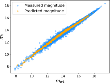
Figure 11. The relation between the i-band apparent magnitudes and w1-band apparent magnitudes of CF4TF.
Download figure:
Standard image High-resolution image
Figure 12. The bottom panel shows the histogram of the i-band absolute magnitudes. The top panel shows the corresponding luminosity function. The blue curve is the Schechter model fit to the data. The green curve is the Schechter model given by Kourkchi et al. (2020a).
Download figure:
Standard image High-resolution imageTo generate mock catalogs for CF4TF, we need to fit the i-band luminosity function for the data. We use the Schechter function (Schechter 1976)

The best-fit values of parameters M⋆ and α are given in the Table 6 of Kourkchi et al. (2020a). However, the shape of the luminosity function given by their parameters cannot match the measurements; see the green curve in the top panel of Figure 12. In addition, Kourkchi et al. (2020a) do not provide the normalization parameter ϕ⋆ of the luminosity function. Therefore, instead of using the values in Table 6 of Kourkchi et al. (2020a), we fit our own luminosity function. The best-fit values are and . The fit result is shown as the blue curve in the top panel of Figure 12.


To emphasize, in this stage we only want to know the shape parameters of the luminosity function; i.e., we only want to know the values of M⋆ and α. The normalization parameter ϕ⋆ is fit in Section 3, as it is difficult to obtain the survey volume of CF4TF due to the complex survey geometry.
Appendix B: The Five CF4TF Patches
In building our mock catalogs, we treat the inhomogeneous CF4TF data as consisting of five distinct patches, each of which has its own unique redshift distribution. Figure 13 shows the five patches of the CF4TF sky coverage we use, which are defined as and correspond to:
- 1.The blue region: 0° < decl. < 38° and 111° < R.A. < 250°. It covers the ALFALFA data in the northern Galactic region.
- 2.The black region: 0° < decl. < 38° and 0° < R.A. < 48° and 3255< R.A. < 360°. It covers the ALFALFA data in the southern Galactic region.
- 3.The green region: decl. > −45°. Here are relatively uniform galaxies, mainly from ADHI, with additions from the Springob/Cornell and Pre-Digital HI catalogs.
- 4.The orange region: 149° < l < 255° and −5° < b < 5°. This has sparse data in the Galactic plane from ADHI, the Springob/Cornell, and Pre-Digital HI catalogs, where Galactic extinction reduces the number density of observed TF objects.
- 5.The red region: decl. < −45°. This includes in the main galaxies from the ADHI but observed using the Parkes Telescope, which results in a lower number density of these galaxies relative to the green region.

Figure 13. The five non-overlapping patches of the CF4TF sky coverage we adopt to produce our mock catalogs.
Download figure:
Standard image High-resolution imageFootnotes
- 3
We use PYTHON function scipy.special.lambertw.
- 4
We use the python package scipy.stats.Gaussian-kde.
- 5
The true log-distance ratio of a mock galaxy is given by , where Dh is calculated from the true position of the mock galaxy. Dm is calculated from its "observed" redshift zm , given by zm = (1 + zt )(1 + vt /c) − 1, where zt is the true redshift calculated from the true position. The term vt is the true line-of-sight velocity of the mock galaxy calculated from its true position and velocity.
- 6
In this method, the galaxies are gridded in using their observed redshifts, and then Equation (2.1.3) of Feldman et al. (1994) and Equation (6) of Bianchi et al. (2015), as well as Equation (11) of Yamamoto et al. (2006), are used to estimate the density power spectrum. This means that we are measuring the redshift space rather than real space power spectrum, which would need to be accounted for if we were performing any theoretical modeling, but avoids the impact of the Malmquist bias or other biases that would arise if one were using the true distances to place the galaxies on the grid.
- 7
The PYTHON package emcee (Foreman-Mackey et al. 2013) is used.
- 8
The corrections are done for Milky Way obscuration, redshift k-correction, and aperture effects as well as global dust obscuration (Kourkchi et al. 2020b).
