


Abstract
We search for signatures of gravitational lensing in the gravitational-wave signals from compact binary coalescences detected by Advanced Laser Interferometer Gravitational-wave Observatory (LIGO) and Advanced Virgo during O3a, the first half of their third observing run. We study: (1) the expected rate of lensing at current detector sensitivity and the implications of a non-observation of strong lensing or a stochastic gravitational-wave background on the merger-rate density at high redshift; (2) how the interpretation of individual high-mass events would change if they were found to be lensed; (3) the possibility of multiple images due to strong lensing by galaxies or galaxy clusters; and (4) possible wave-optics effects due to point-mass microlenses. Several pairs of signals in the multiple-image analysis show similar parameters and, in this sense, are nominally consistent with the strong lensing hypothesis. However, taking into account population priors, selection effects, and the prior odds against lensing, these events do not provide sufficient evidence for lensing. Overall, we find no compelling evidence for lensing in the observed gravitational-wave signals from any of these analyses.
Export citation and abstract BibTeX RIS
1. Introduction
Gravitational lensing occurs when a massive object bends spacetime in a way that focuses light rays toward an observer (see Bartelmann 2010, for a review). Lensing observations are widespread in electromagnetic astrophysics and have been used to, among other purposes, make a compelling case for dark matter (Clowe et al. 2004; Markevitch et al. 2004), discover exoplanets (Bond et al. 2004), and uncover massive objects and structures that are too faint to be detected directly (Coe et al. 2013).
Similarly to light, when gravitational waves (GWs) travel near a galaxy or a galaxy cluster, their trajectories curve, resulting in gravitational lensing (Ohanian 1974; Thorne 1982; Deguchi & Watson 1986; Wang et al. 1996; Nakamura 1998; Takahashi & Nakamura 2003). For massive lenses, this changes the GW amplitude without affecting the frequency evolution (Wang et al. 1996; Dai & Venumadhav 2017; Ezquiaga et al. 2021). Strong lensing, in particular, can also produce multiple images observed at the GW detectors as repeated events separated by a time delay of minutes to months for galaxies (Li et al. 2018; Ng et al. 2018; Oguri 2018), and up to years for galaxy clusters (Smith et al. 2017, 2018, 2019; Robertson et al. 2020; Ryczanowski et al. 2020). The detection of such strongly lensed GWs has been forecast within this decade (Li et al. 2018; Ng et al. 2018; Oguri 2018), at the design sensitivity of Advanced Laser Interferometer Gravitational-wave Observatory (LIGO) and Advanced Virgo, assuming that binary black holes (BBHs) trace the star formation rate density. In addition, if GWs propagate near smaller lenses such as stars or compact objects, microlensing may induce observable beating patterns in the waveform (Deguchi & Watson 1986; Nakamura 1998; Takahashi & Nakamura 2003; Cao et al. 2014; Christian et al. 2018; Dai et al. 2018; Lai et al. 2018; Diego et al. 2019; Jung & Shin 2019; Diego 2020; Pagano et al. 2020; Cheung et al. 2021; Mishra et al. 2021). Indeed, lensing can induce a plethora of effects on GWs.
If observed, GW lensing could enable numerous scientific pursuits, such as localization of merging black holes to subarcsecond precision (Hannuksela et al. 2020), precision cosmography studies (Sereno et al. 2011; Liao et al. 2017; Cao et al. 2019; Li et al. 2019b; Hannuksela et al. 2020), precise tests of the speed of gravity (Baker & Trodden 2017; Fan et al. 2017), tests of the GW's polarization content (Goyal et al. 2021), and detecting intermediate-mass or primordial black holes (Lai et al. 2018; Diego 2020; Oguri & Takahashi 2020).
Here we perform a comprehensive lensing analysis of data from the first half of the third LIGO–Virgo observing run, called O3a for short, focusing on compact binary coalescence (CBC) signals. We begin by outlining the expected rate of strongly lensed events. Strong lensing is rare, but magnified signals enable us to probe a larger comoving volume, thus potentially giving us access to more sources (Dai et al. 2017; Smith et al. 2017, 2018, 2019; Li et al. 2018; Ng et al. 2018; Oguri 2018; Robertson et al. 2020; Ryczanowski et al. 2020). We forecast the lensed event rates using standard lens and black hole population models (Section 3). These expected rates are subject to some astrophysical uncertainty but are vital for the interpretation of our search results in later sections.
The rate of lensing can also be inferred from the stochastic GW background (SGWB; Buscicchio et al. 2020a, 2020b; Mukherjee et al. 2021a). Thus, we use the non-observation of strong lensing and the stochastic background to constrain the BBH merger-rate density and the rate of lensing at high redshifts.
In addition, lensing magnification biases the inferred GW luminosity distance and source mass measurements, which could lead to observations of apparently high-mass (or low-mass, when demagnified) binaries (Dai et al. 2017; Broadhurst et al. 2018, 2020a; Oguri 2018; Hannuksela et al. 2019). Therefore, we analyze several LIGO–Virgo detections with unusually high masses under the alternative interpretation that they are lensed signals from lower-mass sources that have been magnified (Section 4).
We then move on to search for signatures of lensing-induced multiple images, which should appear as repeated similar signals, magnified and with waveform differences determined by the image type (Dai & Venumadhav 2017; Ezquiaga et al. 2021), separated in time by minutes to months (or even years). Consequently, if an event pair is strongly lensed, we expect to infer consistent parameters for both events (Haris et al. 2018; Hannuksela et al. 2019).
We search for these multiple images by first comparing the posterior overlap between pairs of events occurring during the O3a period as reported in Abbott et al. (2021a; Section 5.1). After identifying a list of candidates from the posterior-overlap analysis, we follow these up with more computationally expensive but more accurate joint-parameter estimation (PE) procedures (Section 5.2). Next, we perform a targeted search for previously undetected counterpart images of known events in Section 5.3, images that could have fallen below the threshold of previous wide-parameter space CBC searches (as discussed in Li et al. 2019a; Dai et al. 2020; McIsaac et al. 2020). Finally, we search for microlensing induced by point-mass lenses in the intermediate- and low-mass range, including wave-optics effects (Section 6).
Several searches for GW lensing signatures have already been performed in the data from the first two observing runs O1 and O2 (Hannuksela et al. 2019; Li et al. 2019a; Dai et al. 2020; McIsaac et al. 2020; Pang et al. 2020; Liu et al. 2021), including strong lensing and microlensing effects. We will discuss these previous studies in the appropriate sections. Given the growing interest in GW lensing and the existing forecasts, an analysis of the most recent GW observations for lensing effects is now timely.
The results of all of the analyses in this paper and associated data products can be found in LIGO Scientific Collaboration & Virgo Collaboration (2021). GW strain data and posterior samples for all events from Gravitational-Wave Transient Catalog 2 (GWTC-2) are available (GWOSC 2020) from the Gravitational Wave Open Science Center (Abbott et al. 2021b).
2. Data and Events Considered
The analyses presented here use data taken during O3a by the Advanced LIGO (Aasi et al. 2015) and Advanced Virgo (Acernese et al. 2015) detectors. O3a extended from 2019 April 1 to October 1. Various instrumental upgrades have led to more sensitive data, with median binary neutron star (BNS) inspiral ranges (Allen et al. 2012) increased by a factor of 1.64 in LIGO Hanford, 1.53 in LIGO Livingston, and 1.73 in Virgo compared to O2 (Abbott et al. 2021a). The duty factor for at least one detector to be online was 97%; for any two detectors to be online at the same time it was 82%; and for all three detectors together it was 45%. Further details regarding instrument performance and data quality for O3a are available in Abbott et al. (2021a) and Buikema et al. (2020).
The LIGO and Virgo detectors used a photo- recoil-based calibration (Karki et al. 2016; Cahillane et al. 2017; Viets et al. 2018) resulting in a complex-valued, frequency-dependent detector response with typical errors in magnitude of 7% and 4° in phase (Acernese et al. 2018; Sun et al. 2020) in the calibrated O3a strain data.
Transient noise sources, referred to as glitches, contaminate the data and can affect the confidence of candidate detections. Times affected by glitches are identified so that searches for GW events can exclude (veto) these periods of poor data quality (Abbott et al. 2016a, 2020a; Fiori et al. 2020; Davis et al. 2021; Nguyen et al. 2021). In addition, several known noise sources are subtracted from the data using information from witness auxiliary sensors (Davis et al. 2019; Driggers et al. 2019).
Candidate events, including those reported in Abbott et al. (2021a) and the new candidates found by the searches for subthreshold counterpart images in Section 5.3 of this paper, have undergone a validation process to evaluate if instrumental artifacts could affect the analysis; this process is described in detail in Section 5.5 of Davis et al. (2021). This process can also identify data-quality issues that need further mitigation for individual events, such as subtraction of glitches (Cornish & Littenberg 2015) and nonstationary noise couplings (Vajente et al. 2020), before executing PE algorithms. See Table 5 of Abbott et al. (2021a) for the list of events requiring such mitigation.
The GWTC-2 catalog (Abbott et al. 2021a) contains 39 events from O3a (in addition to the 11 previous events from O1 and O2) with a false-alarm rate (FAR) below two per year, with an expected rate of false alarms from detector noise less than 10% (Abbott et al. 2021a). We neglect the potential contamination in this analysis. These events were identified by three search pipelines: one minimally modeled transient search cWB (Klimenko et al. 2004, 2005, 2006, 2011, 2016) and the two matched-filter searches GstLAL (Messick et al. 2017; Sachdev et al. 2019; Hanna et al. 2020) and PyCBC (Allen 2005; Allen et al. 2012; Dal Canton et al. 2014; Usman et al. 2016; Nitz et al. 2017). Their parameters were estimated through Bayesian inference using the LALInference (Veitch et al. 2015) and Bilby (Ashton et al. 2019; Romero-Shaw et al. 2020; Smith et al. 2020) packages. Both the matched-filter searches and PE use a variety of CBC waveform models which generally combine knowledge from post-Newtonian theory, the effective one-body formalism, and numerical relativity (for general introductions to these approaches, see Blanchet 2014; Damour & Nagar 2016; Palenzuela 2020; Schmidt 2020, and references therein). The analyses in this paper rely on the same methods, and the specific waveform models and analysis packages used are described in each section.
Most of the 39 events from O3a are most probably BBHs, while three (GW190425, GW190426_152155, and GW190814) have component masses below 3 M⊙ (Abbott et al. 2020b, 2020d, 2021a), thus potentially containing a neutron star. We consider these 39 events in most of the analyses in this paper, except in the magnification analysis (Section 4), which concerns only 6 of the more unusual events, and the microlensing analysis (Section 6), which focuses on the 36 clear BBH events only.
Specifically, we use the following input data sets for each analysis. The magnification analysis in Section 4 and posterior-overlap analysis in Section 5.1 start from the Bayesian inference posterior samples released with GWTC-2 (GWOSC 2020). The joint-PE analyses in Section 5.2 and microlensing analysis in Section 6 reanalyze the strain data in short segments around the event times, available from the same data release, with data selection and noise mitigation choices matching those of the PE analyses in Abbott et al. (2021a). In addition, the searches for subthreshold counterpart images in Section 5.3 cover the whole O3a strain data set, using the same data-quality veto choices as in Abbott et al. (2021a) but a strain data set consistent with the PE analyses: the final calibration version of LIGO data (Sun et al. 2020) with additional noise subtraction (Vajente et al. 2020).
3. Lensing Statistics
In this section, we first forecast the number of detectable strongly lensed events (Section 3.1). Then, we infer upper limits on the rate of strongly lensed events using two different methods; the first uses only the nondetection of resolvable strongly lensed BBH events (Section 3.2), while the second leverages additionally the non-observation of the SGWB (Section 3.3; Callister et al. 2020; Abbott et al. 2021c). Since the background would originate from higher redshifts, this second method complements the first method.
Throughout this section, we model the mass distribution of BBHs following the results for the Power Law + Peak model of Abbott et al. (2021d). We consider two distinct models of the BBH merger-rate density. Model A brackets most of the population synthesis results (Boco et al. 2019; Eldridge et al. 2019; Neijssel et al. 2019; Santoliquido et al. 2021) corresponding to Population I and II stars, while Model B assumes the Madau–Dickinson ansatz (Madau & Dickinson 2014) where the rate peaks at a particular redshift. For consistency with previous analyses (e.g., Abbott et al. 2021c), we take the Hubble constant from the Planck 2015 observations to be H0 = 67.9 km s−1 Mpc−1 (Ade et al. 2016). Detailed discussion on both models and their respective parameterization is given in Appendix A. The obtained rates are subject to uncertainty because of their dependence on the merger-rate density, which is model-dependent and only partially constrained. They are nevertheless vital to interpreting our search results in later sections (see Section 5).
3.1. Strong Lensing Rate
We predict the rate of lensing using the standard methods outlined in the literature (Li et al. 2018; Ng et al. 2018; Oguri 2018; Mukherjee et al. 2021b; Wierda et al. 2021; Xu et al. 2021), at galaxy and galaxy-cluster lens mass scales. To model the lens population, we need to choose a density profile and a mass function. We adopt the singular isothermal sphere (SIS) density profile for both galaxies and clusters. Moreover, we use the velocity dispersion function (VDF) from the Sloan Digital Sky Survey (SDSS; Choi et al. 2007) for galaxies and the halo mass function from Tinker et al. (2008) for clusters that have been used in other lensing studies as well (e.g., Oguri & Marshall 2010; Robertson et al. 2020). The SIS profile can well describe galaxies. However, the mass distribution of clusters tends to be more complicated. Nevertheless, Robertson et al. (2020) have demonstrated that the SIS model can reproduce the lensing rate predictions from a study of numerically simulated cluster lenses. Thus, we adopt the same model. Under the SIS model, we obtain two images with different magnifications and arrival times. The rate of strong lensing is
where  is the differential comoving number density of lensing halos in a halo mass shell at lens redshift zl; Dc and Vc are the comoving distance and volume, respectively, at a given redshift;
  is the total comoving merger-rate density at redshift zm; (1+zm) accounts for the cosmological time dilation; p(ρ∣zm) is the distribution of the signal-to-noise ratio (S/N) at a given redshift; and σ is the lensing cross-section (Appendix A). Throughout this section and in Section 3.3 we choose a network S/N threshold of ρc = 8 as a point estimator of the detectability of GW signals. We find it to be consistent with the search results in Abbott et al. (2021a) and in Section 5.3, and we estimate its impact to be subdominant with respect to other sources of uncertainties.
In Table 1, we show our estimates of the relative rate of lensing assuming different models (Models A and B) for the merger-rate density. The results are shown separately for galaxy-scale (G) and cluster-scale (C) lenses. Furthermore, these rates are calculated for events that are doubly lensed and for two cases: when only a single event (i.e., the brighter one) is detected (S), and when both of the doubly lensed events are detected (D). The expected fractional rate of lensing (lensed to unlensed rate), which will be necessary for the multi-image analyses (Section 5), ranges from  –10−4), depending on the merger-rate density assumed. We estimate the fractional rate of observed double (single) events for galaxy-scale lenses in the range of 0.9–4.4 × 10⁻⁴ (2.9–9.5 × 10⁻⁴) when using Model A for the merger-rate density. Similarly, for cluster-scale lenses, the fractional rate is estimated to be in the range of 0.4–1.8 × 10⁻⁴ (1.4–4.1 × 10⁻⁴), much rarer than the rates at galaxy scales. These estimates suggest that observing a lensed double image is unlikely at the current sensitivity of the LIGO–Virgo network of detectors. Nevertheless, at design sensitivity and with future upgrades, standard forecasts suggest that the possibility of observing such events might become significant (Li et al. 2018; Ng et al. 2018; Oguri 2018; Mukherjee et al. 2021b; Wierda et al. 2021; Xu et al. 2021). Our lensing rates are consistent with those predicted for singular isothermal ellipsoid models (e.g., Oguri 2018; Wierda et al. 2021; Xu et al. 2021). The main uncertainty in the rate estimates derives from the uncertainties in the merger-rate density at high redshift.
Table 1. Expected Fractional Rates of Observable Lensed Double Events at Current LIGO–Virgo Sensitivity
| Merger-rate Density | Galaxies | Galaxy Clusters | ||
|---|---|---|---|---|
| Model | RD | RS | RD | RS |
| A | 0.9–4.4 × 10⁻⁴ | 2.9–9.5 × 10⁻⁴ | 0.4–1.8 × 10⁻⁴ | 1.4–4.1 × 10⁻⁴ |
| B | 1.0–23.5 × 10⁻⁴ | 2.5–45.2 × 10⁻⁴ | 0.7–10.9 × 10⁻⁴ | 1.6–19.9 × 10⁻⁴ |
Note. This table lists the relative rates of lensed double events expected to be observed by LIGO–Virgo at the current sensitivity where both of the lensed events are detected (RD) and only one of the lensed events is detected (RS) above the S/N threshold. For Model A, the range corresponds to the bracketing function (see Appendix A) and for Model B, the rates encompass a 90% credible interval. We show the rate of lensing by galaxies (σvd = 10–300 km s−1) and galaxy clusters ( ) separately. Besides their usage for forecasts, the fraction of lensed events allows us to interpret the prior probability of the strong lensing hypothesis, which we require to identify lensed events confidently.
Download table as: ASCIITypeset image
Depending on the specific distribution of lenses and the source population, the time delays between images can change. Models favoring galaxy lensing produce minutes to perhaps months of time delay, while galaxy-cluster lensing can produce time delays even up to years. However, the time-delay distribution for galaxy-cluster lenses is more difficult to model accurately, owing to the more complex lensing morphology.
Since the merger-rate density at high redshift is observationally constrained only by the absence of the SGWB, these rates are subject to uncertainty. Nevertheless, standard theoretical models will still produce useful forecasts. We will later refer to these rate estimates in the relevant sections (see Section 5).
3.2. Implications from the Non-observation of Strongly Lensed Events
Motivated by the absence of evidence for strong lensing (Section 5), we assume that no strong lensing has occurred, in order to constrain the merger-rate density at high redshift. We use the standard constraints on the merger-rate density at low redshift from the LIGO–Virgo population studies (Abbott et al. 2021d). We assume the Madau–Dickinson form for the merger-rate density (Model B). This model's free parameters include the local merger-rate density, the merger-rate density peak, and the power-law slope. The non-observation of lensing constrains the merger-rate density at high redshift, which is unconstrained by the low-redshift observations alone (Figure 1). These lensing constraints are complementary to the current strictest high-redshift limits obtained through SGWB non-observation (Abbott et al. 2021c).
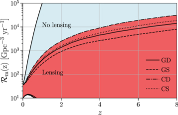
Figure 1. Merger-rate density as a function of redshift based on the GWTC-2 results without lensing constraints (blue) and with lensing (red) included in the LIGO–Virgo detections. We show the results for galaxy-scale lenses (G) and cluster-scale lenses (C) separately. Furthermore, S (or D) corresponds to doubly lensed events where single (or double) events are detected. Because lensed detections occur at higher redshifts than unlensed events, their non-observation can be used to constrain mergers at higher redshifts. The results without lensing do not include constraints derived from the absence of an SGWB.
Download figure:
Standard image High-resolution image3.3. Constraints from Stochastic Background
We can also constrain the redshift evolution of the merger-rate density from the reported non-observation of the SGWB from BBHs (Callister et al. 2020; Abbott et al. 2021c). This, in turn, provides constraints on the relative abundance of distant mergers, which are more likely to undergo lensing. Thus, the non-observation of the SGWB can inform the estimation of the probability of observing lensed BBH mergers (Buscicchio et al. 2020a; Mukherjee et al. 2021a).
Following Buscicchio et al. (2020a), we forecast constraints on the merger-rate density in O3 using up-to-date constraints on the mass distribution and redshift evolution of BBH mergers obtained from the latest detections (Abbott et al. 2019a, 2019b, 2021a, 2021d), as well as those inferred from current upper limits on the SGWB, given its non-observation (Abbott et al. 2021c).
While the measured parameters for each merger (redshifts, source masses) are potentially biased by lensing, as discussed in Section 4, we express all quantities as functions of nonbiased merger redshift zm and chirp mass  (Buscicchio et al. 2020a) for consistency with other sections. However, following Buscicchio et al. (2020a), we do not assume as prior information that lensing is not taking place. Instead, we include the magnification bias self-consistently in the analysis, by imposing population constraints in apparent masses and redshifts.
We model the differential lensing probability following Dai et al. (2017). The differential merger rate in a redshift and magnification shell is
where  is the differential merger-rate density;
  provides the probability of observing mergers with source masses m1, m2, redshift zm, and magnified by a factor μ above a fixed network S/N threshold ρc = 8, integrated over the population distribution of source parameters; the factor
 ![$4\pi {D}_{{\rm{c}}}^{2}({z}_{{\rm{m}}})/[{H}_{0}(1+{z}_{{\rm{m}}})E({z}_{{\rm{m}}})]$](https://content.cld.iop.org/journals/0004-637X/923/1/14/revision1/apjac23dbieqn8.gif) gives the comoving volume of a redshift shell in an expanding universe (taking into account the redshifted rate definition with respect to the source frame); and
gives the comoving volume of a redshift shell in an expanding universe (taking into account the redshifted rate definition with respect to the source frame); and  is the lensing probability. However, as noted by Dai et al. (2017), the differential magnification probability at 0.9 < μ < 1.1 and zm
< 2 is affected by relative uncertainties up to 40%. We therefore consider magnified detections only (μ > 1), which are subject to less uncertainty, and normalize our results accordingly. We then integrate the differential merger rate (Equation (2)) over redshift and magnifications in
is the lensing probability. However, as noted by Dai et al. (2017), the differential magnification probability at 0.9 < μ < 1.1 and zm
< 2 is affected by relative uncertainties up to 40%. We therefore consider magnified detections only (μ > 1), which are subject to less uncertainty, and normalize our results accordingly. We then integrate the differential merger rate (Equation (2)) over redshift and magnifications in ![$\left[\mu ,{\mu }_{\max }\right]$](https://content.cld.iop.org/journals/0004-637X/923/1/14/revision1/apjac23dbieqn10.gif) and divide it by the total rate of magnified detections. By doing so, we obtain the cumulative fraction of detected lensed events at any redshift with magnifications larger than μ.
and divide it by the total rate of magnified detections. By doing so, we obtain the cumulative fraction of detected lensed events at any redshift with magnifications larger than μ.
We show the result in Figure 2. We find the observation of lensed events to be unlikely, with the fractional rate at μ > 2 being  . More significantly magnified events are even more suppressed, with a rate of
  at μ > 30. These estimates suggest that most binary mergers that we observe are not strongly lensed. However, as projected in Buscicchio et al. (2020a) and Mukherjee et al. (2021a), at design sensitivity, the same probability will be enhanced, as a widened horizon will probe the merger-rate density deeper in redshift.
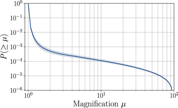
Figure 2. Cumulative fraction of lensed detectable BBH mergers at any redshift with a magnification greater than μ, constrained by the non-observation of the SGWB. The solid line shows the value obtained from the median BBH merger-rate density posterior. The shaded region corresponds to the 90% credible interval. Fewer than 1 in 103 events are expected to be lensed with magnification μ > 2, on average. Significantly higher magnifications (e.g., μ > 30) are suppressed by a further factor of 10. The results here show the probability of observing an event above a given magnification, which includes the merger-rate density and magnification bias information.
Download figure:
Standard image High-resolution imageComparing the above predictions with the expected fractional rates RS of single-lensed detections with Model B in Table 1, the predictions agree within a factor of 5 for the relative rate of lensing. The differences are due to a different underlying lens model and partly to the inclusion of demagnified events in Section 3.1.
4. Analyzing High-mass Events
If a GW signal is strongly lensed, it will receive a magnification μ defined such that the GW amplitude increases by a factor ∣μ∣1/2 relative to an unlensed signal. The luminosity distance inferred from the GW observation will be degenerate with the magnification such that the inferred luminosity distance
Because of this degeneracy, lensing biases the inferred redshift and thus the source masses. Consequently, the binary appears to be closer than it truly is, and it appears to be more massive than it truly is.
Broadhurst et al. (2018, 2020a, 2020b) argued that some of the relatively high-mass LIGO–Virgo events could be strongly lensed GWs from the lower-mass stellar black hole population observed in the electromagnetic bands. However, the expected strong lensing rates and the current constraints on the merger-rate density, based on the absence of a detectable SGWB, disfavor this interpretation (Dai et al. 2017; Li et al. 2018; Ng et al. 2018; Oguri 2018; Hannuksela et al. 2019; Buscicchio et al. 2020a, 2020b) compared to the standard interpretation of a genuine unlensed high-mass population (Abbott et al. 2019a, 2021d; Kimball et al. 2020; Roulet et al. 2020). Hence, in the absence of more direct evidence, such as identifying multiple images within the LIGO–Virgo data (Section 5), it is difficult to support the lensing hypothesis purely based on magnification considerations. Nevertheless, it is informative to analyze the degree to which the lensed interpretation would change our understanding of the observed sources.
Under the strong lensing hypothesis  , the GW would originate from a well-known, intrinsically lower-mass population, and the LIGO–Virgo observations have been biased by lensing. Using such a mass prior, we infer the required magnification and corrected redshift and component masses under
  . The posterior distribution of the parameters is (Pang et al. 2020)

where we distinguish the apparent parameters of the waveform received at the detector ϑ, which differ from the intrinsic parameters θ due to bias by lensing magnification. Therefore, we can compute the magnification posterior and other parameters by simply reweighting existing posteriors.
Studies along these lines were already done for the GW190425 BNS event by Pang et al. (2020) and for the GW190521 BBH event in Abbott et al. (2020e). Here we extend the approach to cover additional interesting O3a events, focusing on two cases: (i) the (apparently) most massive observed BBHs, and (ii) sources with an (apparent) heavy neutron star component. In the BBH case, we take the prior over component masses, m1 and m2, and redshift, z of the source p(m1, m2, z) from the power-law BBH population model used in Abbott et al. (2019a) for O1 and O2 observations, with a mass power-law index of α = 1, a mass ratio power-law index of βq
= 0, and a minimum component mass of  , and assume an absence of BBHs above the pair instability supernova (PISN) mass gap. As in the previous GW190521 study (Abbott et al. 2020e), we consider two different values to account for uncertainties on the edge of the PISN gap,
  . Such a simple model is adequate for this analysis because our analysis results are most sensitive to the mass cut (highest masses allowed by the prior) and less sensitive to the specific shape of the mass distribution. For events with an apparent heavy neutron star component, we assume a Galactic BNS prior following a total mass with a 2.69 M⊙ mean and 0.12 M⊙ standard deviation (Farrow et al. 2019). In both cases, the magnification could explain the apparent high mass of the events from the LIGO–Virgo observations.
We assume that the redshift prior p(z) ∝ τ(z)dVc/dz, where the optical depth of lensing by galaxies or galaxy clusters  (Haris et al. 2018). The redshift dependence of the optical depth is approximately the same for both galaxies and galaxy clusters, while the overall scaling can change (Fukugita & Turner 1991). We use the lensing prior
  (Blandford & Narayan 1986) with a lower limit of μ > 2 appropriate to strong lensing (Ng et al. 2018). This prior is appropriate when we are in the high-magnification, strong lensing limit, i.e., assuming that the observed masses are highly biased. We do not consider weak lensing, which does not produce multiple images and would require expanded future GW data sets to study (Mukherjee et al. 2020a, 2020b).
We analyze all O3a BBH events with the primary mass above 50 M⊙ at 90% probability using the Bayesian inference posterior samples released with GWTC-2 (GWOSC 2020; Abbott et al. 2021a). Moreover, we analyze GW190425, a high-mass BNS (Abbott et al. 2020b), and GW190426_152155, a low-significance potential neutron star–black hole (NSBH) event (Abbott et al. 2021a), which was investigated as a possible lensed BNS event (Smith et al. 2019). We use the results for the IMRPhenomPv2 waveform (Hannam et al. 2014; Bohé et al. 2016) for most of the events. For GW190521, where higher-order multipole moments are important to include in the analysis (Abbott et al. 2020e), we adopt the NRSur7dq4 waveform (Varma et al. 2019) results as in Abbott et al. (2020f). Furthermore, for GW190425 (Abbott et al. 2020b), we use the IMRPhenomPv2_NRTidal (Dietrich et al. 2019) low-spin samples. The results are summarized in Table 2.
Table 2. Inferred Properties of Selected O3a Events under the Lensing Magnification Hypothesis
| Event Name | m1 (M⊙) | m2 (M⊙) | z | μ |
|---|---|---|---|---|
| GW190425 |

|

|

|

|
| GW190426_152155 |

|

|

|

|
| Event Name |
 ( ( ) [M⊙] ) [M⊙] |
 ( ( ) [M⊙] ) [M⊙] | z50 (z65) | μ50 (μ65) |
| GW190521 |
 ( ( ) ) |
 ( ( ) ) |
 ( ( ) ) |
 ( ( ) ) |
| GW190602_175927 |
 ( ( ) ) |
 ( ( ) ) |
 ( ( ) ) |
 ( ( ) ) |
| GW190706_222641 |
 ( ( ) ) |
 ( ( ) ) |
 ( ( ) ) |
 ( ( ) ) |
Note. Under the hypothesis that the listed events are lensed signals from intrinsically lower-mass binary populations with μ > 2, this table lists the favored source masses, redshifts, and magnifications for the BNS and NSBH (top) and BBH (bottom) high-mass events. For the BBHs, two sets of numbers are given for different assumptions about the edge of the pair instability supernova (PISN) mass gap (a cut at 50 M⊙ and 65 M⊙). For the BNSs, we presume that they originate from the Galactic BNS population. To interpret the heavy BBHs as lensed signals originating from the assumed lower-mass population, they should be magnified at a moderate magnification of  at z ∼ 1 to 2. The BNS and NSBH events would require extreme magnifications.
Download table as: ASCIITypeset image
To interpret the heavy BBHs as lensed signals originating from the assumed lower-mass population, they should be magnified at a moderate magnification of μ ∼ 10 at z ∼ 1–2. Depending on the lens model, this magnification may imply a moderate chance of an observable multi-image counterpart as events closer to the caustic curves experience more substantial magnifications. Consequently, they often produce events with similar magnification ratios and shorter time delays (comparable magnifications and shorter time delays can be derived from the lens's symmetry, although if lensing by substructures or microlenses is present, the magnifications between images can differ even in the high-magnification limit). However, we could not identify any multi-image counterparts for any of the high-mass events in our multiple-image search (Section 5).
The BNS and NSBH events, on the other hand, would require extreme magnifications ( and
and  , respectively) to be consistent with the Galactic BNS distribution. At these magnifications, we would expect the source to be close to a caustic, and therefore it may be possible that the presence of microlenses would produce observable effects (Diego et al. 2019; Diego 2020; Pagano et al. 2020; Mishra et al. 2021). Moreover, the event would likely be multiply imaged (Blandford & Narayan 1986; Oguri 2018). A more detailed follow-up study to quantify the likelihood of multiple images and microlensing could produce more stringent evidence for the lensing hypothesis for these events. We will briefly comment on these events in the context of multi-image and microlensing results in the sections that follow.
At this stage, we cannot set robust constraints on the lensing hypothesis based on the magnification alone. Moreover, as detailed in the following section, we have also not found any other clear evidence to indicate that these GW events are lensed. The prior lensing rate disfavors the lensing hypothesis for most standard binary population and lens models, as discussed in Section 3. However, if other BBH formation channels exist that produce an extensive number of mergers at high redshift, the lensing rates can change. In the future, more quantitative constraints could be set by connecting the inferred magnifications with lens modeling to make predictions for the appearance of multiple images or microlensing effects.
5. Search for Multiple Images
In addition to magnification, strong lensing can produce multiple images of a single astrophysical event. These multiple images appear at the GW detectors as repeated events. The images will differ in their arrival time and amplitude (Wang et al. 1996; Haris et al. 2018; Hannuksela et al. 2019; Li et al. 2019a; McIsaac et al. 2020). The sky location is the same within the localization accuracy of GW detectors, given that the typical angular separations are of the order of arcseconds. Additionally, lensing can invert or Hilbert transform the image (Dai & Venumadhav 2017; Ezquiaga et al. 2021), introducing a frequency-independent phase shift. This transformation depends on the image type, set by the lensing time delay at the image position: Type-I, II, and III correspond to a time-delay minimum, saddle point, and maximum, respectively (Ezquiaga et al. 2021).
The multiply imaged waveforms  of a single signal
  then satisfy (Dai & Venumadhav 2017; Ezquiaga et al. 2021)
where  is the lensing magnification experienced by the image j and Δϕj
= − π
nj
/2 is the Morse phase, with indices of nj
= 0, 1, 2 for Type-I, II, and III images.
is the lensing magnification experienced by the image j and Δϕj
= − π
nj
/2 is the Morse phase, with indices of nj
= 0, 1, 2 for Type-I, II, and III images.  is the original (unlensed) waveform before lensing, but evaluated as arriving with a time delay Δtj
. The multi-image hypothesis then states that most parameters measured from the different lensed images of the same event are consistent.
is the original (unlensed) waveform before lensing, but evaluated as arriving with a time delay Δtj
. The multi-image hypothesis then states that most parameters measured from the different lensed images of the same event are consistent.
The relative importance of different parameters for the overall consistency under the multi-image hypothesis will vary for different events. For example, the sky localization match will have greater relevance for well-localized, high-S/N events. Similarly, the overlap in measured chirp mass  will be more significant when the uncertainty in that parameter is lower, although in this case the underlying astrophysical mass distribution will play a key role. The similarities in other parameters such as mass ratios or spins will be more important when they depart from the more common astrophysical expectations. Evidence of strong lensing could also be acquired with a single Type-II (saddle point) image if the induced waveform distortions in the presence of higher modes, precession, or eccentricity are observed (Ezquiaga et al. 2021). Such evidence is unlikely to be observed without next-generation detectors (Wang et al. 2021).
In this section, we perform three distinct but related analyses. First, we test the lensed multi-image hypothesis by analyzing, for all pairs of O3a events from GWTC-2, the overlap of posterior distributions previously inferred for the individual events. This allows us to set ranking statistics to identify an initial set of candidates for lensed multiple images. We perform a more detailed joint-PE analysis for these most promising pairs, considering all potential correlations in the full parameter space and the image type. This joint analysis provides a more solid determination of the lensing probability for a given GW pair. Finally, we search for additional subthreshold candidates that could be multiply imaged counterparts to the previously considered events: some counterpart images can have lower relative magnification compared with the primary image and/or fall in times of worse detector sensitivity or antenna patterns, and hence may not have passed the detection threshold of the original broad searches. According to the predictions of the expected lensing time delays and the rate of galaxy and galaxy-cluster lensing (Oguri 2018; Smith et al. 2018; Dai et al. 2020), we expect it to be less likely for counterpart images of the O3a events to be detected in observing runs O1 or O2. Relative lensing rates for galaxies and clusters are given in Table 1. Thus, we only search for multiple images within O3a itself.
Previous studies have also searched for multiple images in the O1–O2 catalog GWTC-1 (Broadhurst et al. 2019; Hannuksela et al. 2019; Li et al. 2019a; Dai et al. 2020; McIsaac et al. 2020; Liu et al. 2021). The first search for GW lensing signatures in O1 and O2 focused on the posterior overlap of the masses, spins, binary orientation and sky positions (Hannuksela et al. 2019), and the consistency of time delays with expectations for galaxy lenses, but found no conclusive evidence of lensing. The search did uncover a candidate pair GW170104–GW170814 with a relatively high Bayes factor of ≳200. Still, this study disfavored the candidate due to its long time delay and the low prior probability of lensing. In parallel, Broadhurst et al. (2019) suggested that the candidate pair GW170809–GW170814 could be lensed, but this claim is disfavored by more comprehensive analyses (Hannuksela et al. 2019; Liu et al. 2021). Both Li et al. (2019a) and McIsaac et al. (2020) performed searches for subthreshold counterparts to the GWTC-1 events, identifying some marginal candidates but finding no conclusive evidence of lensing. More recently, Dai et al. (2020) and Liu et al. (2021) searched for lensed GW signals including the analysis of the lensing image type, which can be described through the Morse phases, Δϕj in Equation (5). These analyses have revisited the pair GW170104–GW170814 and demonstrated that the Morse phase is consistent with the lensed expectation but would require Type-III (time-delay maximum) images, which are rare from an observational standpoint. Dai et al. (2020) also pointed out that a subthreshold trigger, designated by them as GWC170620, is also consistent with coming from the same source. However, the required number and type of images for this lens system make the interpretation unlikely given current astrophysical expectations. Also, two same-day O3a event pairs (on 2019 May 21 and August 28) have already been considered elsewhere, but were both ruled out due to vanishing localization overlap (Singer et al. 2019; Abbott et al. 2020e).
5.1. Posterior-overlap Analysis
As a consequence of degeneracies in the measurements of parameters, the lensing magnification can be absorbed into the luminosity distance (Section 4), the time delay can be absorbed into the time of coalescence, and, when the radiation is dominated by ℓ = ∣m∣ = 2 multipole moments, the phase shifts introduced by lensing (the Morse phases) can be absorbed into the phase of coalescence. The multi-image hypothesis then states that all other parameters except the arrival time, luminosity distance, and coalescence phase are the same between lensed events, and thus there should be extensive overlap in their posterior distributions, even if those have been inferred without taking lensing into account.
Therefore, we use the consistency of GW signals detected by LIGO and Virgo to identify potential lensed pairs. Following Haris et al. (2018), we define a ranking statistic  to distinguish candidate lensed pairs from unrelated signals,

where the parameters Θ include the redshifted masses (1 + z)m1,2, the dimensionless spin magnitudes χ1,2, the cosine of spin tilt angles θ1,2, the sky location  , and the cosine of orbital inclination θJN
, but they do not include the full fifteen-dimensional set of parameters Θ to ensure the accuracy of the kernel density estimators (KDEs) that we use to approximate the posterior distributions p(Θ∣d1,2) for each event when evaluating Equation (6). Here, p(Θ) denotes the prior on Θ.
, and the cosine of orbital inclination θJN
, but they do not include the full fifteen-dimensional set of parameters Θ to ensure the accuracy of the kernel density estimators (KDEs) that we use to approximate the posterior distributions p(Θ∣d1,2) for each event when evaluating Equation (6). Here, p(Θ) denotes the prior on Θ.
The accuracy of the KDE approximation was demonstrated in Haris et al. (2018) through receiver operating characteristic curves with simulated lensed and unlensed BBH events. To improve the accuracy further, we compute the sky localization (α, δ) overlap separately from other parameters and combine it with the overlap from the remaining parameters. Splitting the two overlap computations is justified because the posterior correlations of (α, δ) with other parameters are minimal.
We use posterior samples (GWOSC 2020) obtained using the LALInference software package (Veitch et al. 2015) with the IMRPhenomPv2 waveform model (Hannam et al. 2014; Bohé et al. 2016) for most of the events. However, for GW190521, we use NRSur7dq4 (Varma et al. 2019) posteriors, and for GW190412 and GW190814 we use IMRPhenomPv3HM (Khan et al. 2020) posteriors. The prior p(Θ) is chosen to be uniform in all parameters. The component mass priors have the bound (2–200 M⊙). Equation (6) then quantifies how consistent a given event pair is with being lensed. In our analysis, we omit the BNS event GW190425 (Abbott et al. 2020b) because it was detected at relatively low redshift, and hence we expect the probability of it being lensed to be very small.
In addition to the consistency of the frequency profile of the signals (as measured by the posterior overlap), the expected time delays Δt between lensed images follow a different distribution than for pairs of unrelated events. Following Haris et al. (2018), we define
where  and
and  are the prior probabilities of the time delay Δt under the strongly lensed and unlensed hypotheses, respectively. Here
  is obtained by assuming that the GW events follow a Poisson process. We use a numerical fit to the time-delay distribution
  obtained in Section 3 for the SIS galaxy lens model, with a merger-rate density given by Rmin in Equation (A1). Equation (7) provides another ranking statistic to test the lensing hypothesis, based on the time delay, though subject to some astrophysical uncertainties (see the discussion in Section 3). The time-delay distribution does not include galaxy-cluster lenses, which may be responsible for long time delays of several months or more. We also do not model detector downtime, but we expect the different contributions to the time delay to average out across a longer time period.
To estimate the significance of the combined ranking statistic,  computed for O3a event pairs, we perform an injection campaign. For the injection campaign, we sample component masses m1,2 from a power-law distribution (Abbott et al. 2016b) in the range of (10–50 M⊙). We assume that the redshift distribution follows population synthesis simulations of isolated binary evolution (Belczynski et al. 2008, 2010; Dominik et al. 2013; Marchant et al. 2018; Boco et al. 2019; Eldridge et al. 2019; Neijssel et al. 2019; Santoliquido et al. 2021); in particular, for illustration purposes, we show results using the redshift evolution from Belczynski et al. (2016a, 2016b), but for the local universe that we look at (z < 2), other models produce qualitatively similar results. All other parameters are sampled from uninformative prior distributions (Haris et al. 2018). We inject the simulated signals into Gaussian noise with O3a representative spectra for a LIGO–Virgo detector network. We compute
  and
and  for all possible pairs in the injection set to obtain the false-alarm probability for one pair FAPpair(x) at different levels x of combined statistics by counting the number of simulated pairs with
  . Then the probability of at least one of the N event pairs in GWTC-2 to cross the threshold can be estimated as
 ![${\mathrm{FAP}}^{\mathrm{cat}}(x)=1-{[{\mathrm{FAP}}^{\mathrm{pair}}(x)]}^{N}$](https://content.cld.iop.org/journals/0004-637X/923/1/14/revision1/apjac23dbieqn73.gif) . We then obtain the σ levels of significance shown in Figure 3 by assuming FAPcat(x) follows the complementary error function.
. We then obtain the σ levels of significance shown in Figure 3 by assuming FAPcat(x) follows the complementary error function.

Figure 3. Scatter plot of the ranking statistics  and
and  for a subset of event pairs that have both
  and
and  . The dashed lines denote the significance levels of the combined ranking statistics (in terms of Gaussian standard deviations), obtained by simulating unlensed event pairs in Gaussian noise matching the O3a sensitivity of the LIGO–Virgo network. We identify several high
  candidates, which we follow up on with a detailed joint-PE analysis. We have used abbreviated event names, quoting the last four digits of the date identifier (see Table 3 for full names).
Download figure:
Standard image High-resolution imageIn Figure 3 we show the scatter plot of  and
and  for the O3a event pairs that have a high combined ranking statistic. The dashed lines represent different significance levels as obtained from the simulations. The event pair GW190728_064510–GW190930_133541 gives the highest combined ranking statistic,
  however, as can be seen from Figure 3, its significance is above 1σ (68%) but much below the 2σ (95%) significance level.
To follow up on the most promising event pairs with the more detailed joint-PE analysis in the next section, we make a selection based on just the posterior-overlap ranking statistic,  , rather than the combined ranking statistic,
  , because
  depends strongly on the lens model. That is, we do not rule out any candidates based on
  . Our aim in the next section is to understand the high
  event pairs in greater detail without resorting to any specific lens model. We thus select the most promising event pairs from Figure 3, i.e., those with
  , and carry out the joint-PE analysis in the next section. The 19 selected pairs are listed in Table 3.
Table 3. Summary of Joint-PE Results for Event Pairs in O3a

|

|

| |||
|---|---|---|---|---|---|
| Event 1 | Event 2 |

| LALInference | hanabi | hanabi |
| (Δϕ: 0, π/2, π, 3π/2) | |||||
| GW190412 | GW190708_232457 | −1.6 |

| −6.6 | −9.7 |
| GW190421_213856 | GW190910_112807 | − |

| −0.7 | − 3.8 |
| GW190424_180648 | GW190727_060333 | −1.8 |

| −0.8 | − 3.9 |
| GW190424_180648 | GW190910_112807 | − |

| −0.8 | − 3.9 |
| GW190513_205428 | GW190630_185205 | −0.6 |

| −2.4 | − 5.5 |
| GW190706_222641 | GW190719_215514 | + 0.4 |

| −0.3 | −3.4 |
| GW190707_093326 | GW190930_133541 | −1.5 |

| −9.4 | −12.5 |
| GW190719_215514 | GW190915_235702 | −0.9 |

| −0.7 | − 3.8 |
| GW190720_000836 | GW190728_064510 | + 0.5 |

| −6.7 | −9.8 |
| GW190720_000836 | GW190930_133541 | −1.2 |

| −9.2 | −12.3 |
| GW190728_064510 | GW190930_133541 | −1.1 |

| −8.5 | −11.6 |
| GW190413_052954 | GW190424_180648 | + 0.4 |

| −1.6 | −4.7 |
| GW190421_213856 | GW190731_140936 | −2.1 |

| −0.2 | − 3.3 |
| GW190424_180648 | GW190521_074359 | −0.1 |

| −2.0 | − 5.1 |
| GW190424_180648 | GW190803_022701 | −2.1 |

| −1.0 | − 4.1 |
| GW190727_060333 | GW190910_112807 | −0.6 |

| −1.4 | −4.5 |
| GW190731_140936 | GW190803_022701 | + 0.9 |

| −0.9 | − 4.0 |
| GW190731_140936 | GW190910_112807 | −0.5 |

| −1.2 | − 4.3 |
| GW190803_022701 | GW190910_112807 | −0.4 |

| −0.1 | − 3.2 |
Note. We select those events with a posterior-overlap ranking statistic larger than 50. For each pair of events presented in the first two columns, the third column lists the time-delay ranking statistic  as described in Section 5.1. The next column gives the coherence ratio of the lensed/unlensed hypothesis
  obtained with the LALInference-based pipeline, including the results for the four possible lensing phase differences Δϕ = 2Δϕc. We highlight in bold those pairs with
  for at least one Morse phase shift. The fifth and sixth columns correspond to the hanabi results for the population-weighted coherence ratio
  and the Bayes factor
  . All quantities are given in log10. All high-coherence ratio events display a small Bayes factor when including the population priors and selection effects. For the pairs GW190421_213856–GW190910_112807 and GW190424_180648–GW190910_112807, the time delays between events are larger than what we expect for galaxy lenses in our simulation, and thus
  .
.
Download table as: ASCIITypeset image
5.2. Joint Parameter Estimation Analysis
Here we follow up on the most significant pairs of events from the posterior-overlap analysis with a more detailed but more computationally demanding joint-PE analysis. The benefit of this analysis is that it allows for more stringent constraints on the lensing hypothesis by investigating potential correlations in the full parameter space of BBH signals, instead of marginalizing over some parameters. Moreover, it also includes a test for the lensing image type by incorporating lensing phase information.
We perform our analysis using two independent pipelines, a LALInference-based pipeline (Liu et al. 2021) and a Bilby-based pipeline (hanabi; Lo & Magaña Hernandez 2021), giving us additional confidence in our results. Unlike the posterior-overlap analysis, the joint-PE analysis does not start from existing posterior samples. Instead, we start the inference directly using the detector strain data. In both pipelines, we follow the same data selection choices (calibration version, available detectors for each event, and noise subtraction procedures) as in the original GWTC-2 analysis (Abbott et al. 2021a), with special noise mitigation steps (glitch subtraction and frequency range limitations) taken for some events, as listed in Table 5 of that paper. However, the two pipelines use different waveform models. In this section, we first describe how we quantify the evidence for the strong lensing hypothesis, then detail the two pipelines and finally present the results.
5.2.1. The Coherence Ratio and the Bayes Factor
There will be three types of outputs for the joint-PE analysis. First, we compute a coherence ratio  , which is the ratio of the lensed and unlensed evidences, neglecting selection effects and using default priors in the joint-PE inference. We treat this as a ranking statistic, which quantifies how consistent two signals are with the lensed hypothesis. Large coherence ratios indicate that the parameters of the GWs agree with the expectations of multiple lensed events. This occurs, for example, when the masses and sky localization coincide. However, the coherence ratio does not properly account for the possibility that the parameters overlap by chance.
The likelihood that GW parameters overlap by chance sensitively depends on the underlying population of sources and lenses. For example, if there existed formation channels that produced GWs with similar frequency evolutions (as expected of lensing), the likelihood of an unlensed event mimicking lensing would increase substantially. Thus, we introduce a second output, the population-weighted coherence ratio  , which incorporates prior information about the populations of BBHs and lenses. The value of
  is subject to the choice of both the BBH and lens models.
Similarly, the probability that two signals agree with the multiple-image hypothesis is altered through selection effects, as some masses and sky orientations are preferentially detected. Thus, we also include the selection effects, which gives us our final output, the Bayes factor  .
.  quantifies the evidence of the strong lensing hypothesis for a given detector network and population model. For the full derivations and detailed discussion on the difference between the coherence ratio and the Bayes factor, see Lo & Magaña Hernandez (2021).
5.2.2. LALInference-based Pipeline
For the LALInference-based pipeline, we adopt the method presented by Liu et al. (2021), which was first used for analyzing pairs of events from GWTC-1 (Abbott et al. 2019b). LALInferenceNest (Veitch et al. 2015) implements nested sampling (Skilling 2006), which can compute evidences without explicitly carrying out the high-dimensional integral while sampling the posteriors. The LALInference-based pipeline uses the IMRPhenomD waveform (Husa et al. 2016; Khan et al. 2016), which is a phenomenological model that includes the inspiral, merger, and ringdown phases but assumes nonprecessing binaries and only ℓ = ∣m∣ = 2 multipole radiation. This is motivated by the fact that most events detected so far are well described by the dominant multipole moment (Abbott et al. 2019b, 2021a). Higher-order multipole moments, precession, or eccentricity could lead to nontrivial changes to the waveform for Type-II images, but such waveforms cannot currently be used with this pipeline. For a discussion of the events within GWTC-2 displaying measurable higher-order multipole moments or precession, see Appendix A of Abbott et al. (2021a).
As in the posterior-overlap analysis, we expect observed, lensed GWs to share the same parameters for the redshifted masses, spins, sky position, polarization angle, and inclination, {(1 + z)m1, (1 + z)m2, χ1, χ2, α, δ, ψ, θJN
}. Hence, we force these parameters to be identical under the lensing hypothesis. For the unlensed hypothesis, we sample independent sets of parameters for each event. This is equivalent to performing two separate nested sampling runs and then combining their evidence. In total, LALInference samples in an eleven-dimensional parameter space and provides  as the output.
We sample the apparent luminosity distance of the first event DL
1 and the relative magnification μr (Wang et al. 1996) instead of the luminosity distance of the second event DL
2, using the relation  . Since our waveform only includes the dominant ℓ = ∣m∣ = 2 multipole moments, the lensing Morse phase is modeled by discrete shifts in the coalescence phase ϕc by an integer multiple of π/4 (with relation to the lensing phase shift Δϕ = 2Δϕc; Dai & Venumadhav 2017; Ezquiaga et al. 2021). Thus, we consider all possible relative shifts Δϕc ∈ {0, π/4, π/2, 3π/4} between two GW signals.
We set a uniform prior in ![$\mathrm{log}[(1+z){m}_{1}]$](https://content.cld.iop.org/journals/0004-637X/923/1/14/revision1/apjac23dbieqn124.gif) and
and ![$\mathrm{log}[(1+z){m}_{2}]$](https://content.cld.iop.org/journals/0004-637X/923/1/14/revision1/apjac23dbieqn125.gif) for both the lensed and unlensed hypothesis. The minimum and maximum component masses are respectively 3 M⊙ and 330 M⊙, with a minimum mass ratio of q = m2/m1 = 0.05. This choice reduces the prior volume by 102 − 103 compared to the uniform prior used in GWTC-2 (see Liu et al. 2021, for discussion). For the other parameters, the prior for the luminosity distance is
for both the lensed and unlensed hypothesis. The minimum and maximum component masses are respectively 3 M⊙ and 330 M⊙, with a minimum mass ratio of q = m2/m1 = 0.05. This choice reduces the prior volume by 102 − 103 compared to the uniform prior used in GWTC-2 (see Liu et al. 2021, for discussion). For the other parameters, the prior for the luminosity distance is  up to 20 Gpc, while the spins are taken to be parallel to the dimensionless orbital angular momentum with a uniform prior on the z components between −0.99 (anti-aligned) and +0.99 (aligned).
5.2.3. The hanabi Pipeline
The hanabi pipeline, on the other hand, adopts a hierarchical Bayesian framework that models the data generation process under the lensed and the unlensed hypothesis. This pipeline uses the IMRPhenomXPHM waveform (Pratten et al. 2021), which models the full inspiral–merger–ringdown for generic precessing binaries including both the dominant and some subdominant multipole moments. Therefore, the parameter space of hanabi enlarges to 15 dimensions.
hanabi differs from the LALInference-based pipeline in the treatment of the Morse phase. Here the lensing phase is directly incorporated in the frequency-domain waveform, accounting for any possible distortion of Type-II images (Dai et al. 2017; Ezquiaga et al. 2021; Lo & Magaña Hernandez 2021). Moreover, the lensed probability is computed by considering all possible combinations of image types with a discrete uniform prior (Lo & Magaña Hernandez 2021). For this reason, hanabi only produces one evidence per pair, and not one for each discrete phase difference as in the LALInference-based pipeline. Unlike the LALInference-based pipeline, hanabi samples the observed masses in a uniform distribution. The mass ranges are different for each event pair, but an overall reweighting is applied later (see below). The rest of the prior choices for the intrinsic parameters are the same as for the LALInference-based pipeline with the addition of a discrete uniform prior on the Morse phase and isotropic spin priors.
In addition to computing the joint-PE coherence ratio, hanabi also incorporates prior information about the lens and BBH populations, as well as selection effects. In particular, the BBH population is chosen to follow a Power Law + Peak model in the primary mass following the best-fit parameters in Abbott et al. (2021d). Similarly, the secondary mass is fixed to a uniform distribution between the minimum and the primary mass. hanabi also uses an isotropic spin distribution and merger-rate history following Model A in Section 3. The lens population is modeled by the optical depth described in Hannuksela et al. (2019) and a magnification distribution of p(μ) ∝ μ−3 for μ ≥ 2. hanabi is thus able to output  ,
,  , and
, and  . However, hanabi does not include any preference for a particular type of image, i.e., hanabi uses a discrete, uniform prior for the Morse phase shift Δϕj
.
. However, hanabi does not include any preference for a particular type of image, i.e., hanabi uses a discrete, uniform prior for the Morse phase shift Δϕj
.
5.2.4. Results
Within the O3a events, the LALInference-based pipeline finds 11 pairs with  , indicating high parameter consistency. We have checked that the results of the LALInference-based pipeline are qualitatively consistent with those from hanabi. This reinforces our previous argument that the shift in the coalescence phase is a good approximate description of the lensing Morse phase given that in the present catalog most events are dominated by the ℓ = ∣m∣ = 2 multipole moments. However, because of the pair-dependent prior choices of hanabi, we do not present its raw
  results in Table 3.
We then include our prior expectation on the properties of the lensed images (derived from our BBH and lens population priors) and the selection effects when computing the population-weighted hanabi coherence ratio and the Bayes factors  . The results are summarized in Table 3. The event pair GW190728_064510–GW190930_133541, which seemed the most promising from the overlap analysis in Section 5.1, is disfavored by both of the joint-PE pipelines. After the inclusion of the population prior and selection effects, none of the event pairs display a preference for the lens hypothesis (
 ).
).
The population-weighted coherence ratio and the Bayes factor are subject to the BBH and lens model specifications. The population properties are not inferred taking into account the possibility of lensing. This introduces an inevitable bias, but it can be justified a posteriori to be a good approximation given the expected low rate of strong lensing. Additionally, the population properties include significant uncertainties in the hyper-parameter estimates and presume a population model. In any case, to quantify this intrinsic uncertainty in the modeling, we consider different choices for the mass distribution and merger-rate history. Varying the maximum BBH mass and the redshift evolution of the merger rate using the  and
and  of Model A in Section 3, we find that the strong lensing hypothesis is always disfavored. While these results are subject to assumptions on prior choices, our results are sufficient to reject the strong lensing hypothesis: even if other prior choices favored the lensing hypothesis, the evidence would be inconclusive at best.
The impact of the selection effects is considerable. Among other reasons, this is because present GW detectors preferentially observe higher-mass events (Fishbach & Holz 2017), making coincidences in observed masses more probable. Along the same lines, given the specific antenna patterns of the current network of detectors, GW events are preferentially seen in specific sky regions with characteristic elongated localization areas (Chen et al. 2017), which favors the overlap between different events.
We also reanalyze the GW170104–GW170814 event pair in the O2 data previously studied by Dai et al. (2020) and Liu et al. (2021). Using the LALInference-based pipeline, Liu et al. (2021) found that the coherence ratio, including selection effects associated with the Malmquist bias (Malmquist 1922), is  for a π/2 coalescence phase shift. However, when including together the population and selection effects with hanabi, we find that the evidence drastically reduces to a Bayes factor of
  .
.
In addition to the Bayes factor, it is important to contrast the recovered number of candidate lensed pairs and their properties with astrophysical expectations. In Section 3.1 we found that the relative rate of GW events with at least two strongly lensed images above the detection threshold is below ∼1.3 × 10⁻³ for all considered BBH population models. Thus, the lensing rate estimates significantly disfavor the lensing hypothesis a priori; even a moderate Bayes factor by itself would not yet make a compelling case for strong lensing. Additionally, the type of images, arrival times, and magnifications provide additional information on the lensing interpretation's plausibility. For example, a quantification of the time-delay prior can be computed by multiplying the coherence ratio by  . However, our final conclusions do not depend on the prior information about the lensing time delays or the prior odds against lensing: the prior lensing knowledge further disfavors the strong lensing hypothesis, but we did not use it to rule out any candidates.
Although we do not find evidence of strong lensing, future electromagnetic follow-up of the candidates could allow for independent support for the hypothesis if we identified a lensed counterpart galaxy to these events (Sereno et al. 2011; Smith et al. 2017, 2018, 2019; Hannuksela et al. 2020; Robertson et al. 2020; Ryczanowski et al. 2020; Yu et al. 2020). This identification could take place by matching GW and electromagnetic image properties when four GW images are available (Hannuksela et al. 2020). With two images, the number of hosts could also be constrained (Sereno et al. 2011; Yu et al. 2020), but to a lesser degree due to degeneracies with the lens and source alignment and uncertainties introduced by micro/millilensing—although strong lensing by galaxy clusters might allow us to identify a single cluster candidate (Smith et al. 2017, 2018, 2019; Robertson et al. 2020; Ryczanowski et al. 2020). Moreover, strong lensing could have produced additional images below the noise threshold. We perform a further investigation of such subthreshold counterparts in the next section.
5.3. Search for Subthreshold Lensed Images
Here we search for subthreshold counterpart images of the O3a events from GWTC-2 that would not have been identified as confident detections by the search pipelines used in Abbott et al. (2021a). As lensed images could in principle appear anywhere in the entire O3a data, we perform targeted template bank searches for these subthreshold lensed counterparts over the whole O3a strain data set, following the data selection criteria described in Abbott et al. (2021a). We employ two matched-filter searches based on the GstLAL (Cannon et al. 2012; Messick et al. 2017; Sachdev et al. 2019; Hanna et al. 2020) and PyCBC (Usman et al. 2016; Nitz et al. 2018, 2019; Davies et al. 2020) pipelines, adapted to the lensing case in similar ways as in Li et al. (2019a) and McIsaac et al. (2020).
5.3.1. Search Methods and Setups
The lensed hypothesis states that the intrinsic masses and spins will remain consistent between multiple lensed images of the same event. Hence, we can perform searches that specifically target subthreshold lensed counterparts of known events by creating reduced banks of template waveforms with masses and spins close to those inferred for the primary event. We use the public posterior mass and spin samples released with GWTC-2 (GWOSC 2020) to create these targeted template banks. This ensures that the known events will match well with the templates while simultaneously decreasing the FAR of the search for similar events, potentially returning new candidates that did not reach the search threshold in Abbott et al. (2021a). The reduced banks of GstLAL contain between 173 and 2698 templates per search, while for each PyCBC search we select a single aligned-spin template. The construction of these template banks closely follows Li et al. (2019a) and McIsaac et al. (2020) and is detailed further in Appendix B. Template waveforms are generated using the aligned-spin SEOBNRv4_ROM waveform (Pürrer 2014, 2016; Bohé et al. 2017) for both pipelines and all events, with the exception of GW190425 in the PyCBC search, where we use the TaylorF2 model (Sathyaprakash & Dhurandhar 1991; Blanchet et al. 1995, 2005; Poisson 1998; Damour et al. 2000; Mikoczi et al. 2005; Arun et al. 2009; Buonanno et al. 2009; Faye et al. 2012; Bohé et al. 2013, 2015; Blanchet 2014; Mishra et al. 2016).
Given these template banks, each search pipeline proceeds with configurations and procedures as outlined in Abbott et al. (2021a) to produce a priority list of potential lensed candidates matching each target event. To rank these, each pipeline uses a different method to estimate FARs.
GstLAL first identifies matched-filter triggers from one or more of the Hanford, Livingston, and Virgo data streams. Coincidences are identified with the same settings as in Abbott et al. (2021a). From each candidate's recovered parameters, a likelihood-ratio ranking statistic is computed (Sachdev et al. 2019). Single-detector triggers are penalized using machine-learning-based predictions (iDQ; Essick et al. 2020; Godwin et al. 2020) whereas for coincident triggers, no data-quality products are used. We estimate the FAR of a trigger by comparing it with the distribution of the ranking statistic from all noncoincident noise triggers, used to characterize the noise distribution, over the O3a data set.
PyCBC also first identifies single-detector matched-filter triggers, with a reduced clustering window compared to the GWTC-2 configuration (from 1 to 0.01 s). These are tested for time coincidence between detectors and are required to have an S/N≥ 4 in at least two detectors. While in the GWTC-2 analysis the PyCBC search was limited to the Hanford and Livingston detectors, here we also include Virgo data, using the methods described in Davies et al. (2020) to analyze the three-detector network. FARs are estimated from a noise background measured using time-shifted data. All triggers within 0.1 s of the times of the events in GWTC-2 are removed from both the foreground (observed coincident events) and the background.
Candidates from both pipelines are further vetted by a sky localization consistency test against the targeted GWTC-2 event, as lensed images of the same event should come from consistent sky locations, but the matched-filter searches do not check for this. For each new candidate, we generate a sky localization map p(Ω) using Bayestar (Singer & Price 2016), with Ω denoting parameters that specify the sky location. We compute the percentage of the overlap O90%CR of the 90% credible regions between the sky localization q(Ω) of a GWTC-2 event and the sky localization p(Ω) of a subthreshold event candidate as

where 1 is the indicator function. To avoid false dismissal at this step, we only veto candidates with O90%CR = 0. All candidates with nonvanishing localization overlap are kept for further follow-up with data-quality checks as discussed in Section 2 and with the joint-PE methods described in Section 5.2.
5.3.2. Results
In Table 4, we list the 8 candidates with FAR < 1 in 16 years from the individual targeted searches for counterparts of the 39 detections reported in GWTC-2 found by at least one pipeline. Six of these are unique candidates. This number, compared with ∼2 expected noise events above this FAR from the number of searches performed, is consistent with additional astrophysical signals being present in the data set. However, in this work, we do not assess in detail the probability of astrophysical origin for each of these. The reported FARs also do not indicate how likely each trigger is to be a lensed counterpart of the targeted event, but only how likely it is to obtain a trigger with a similar ranking statistic from a pure noise background using these reduced template banks. Three of these candidates were also recovered with high probability of an astrophysical origin in the third Open Gravitational-wave Catalog (3-OGC) open-data search (Nitz et al. 2021), which used a broad template bank. Five of them are also included with pastro > 0.5 in the extended catalog of GWTC-2.1 (Abbott et al. 2021e). Candidates matching one or both of these catalogs are marked within the footnotes of Table 4.
Table 4. Candidates from Individual Subthreshold Searches for Strongly Lensed Counterpart Images of the 39 O3a Events from GWTC-2
| UTC Time | GWTC-2 Targeted Event | ∣Δt∣ (days) |

| FAR 
| O90%CR (%) |
 (LALInference) (LALInference) | |
|---|---|---|---|---|---|---|---|
| (M⊙) | PyCBC | GstLAL | (Δϕ: 0, π/2, π, 3π/2) | ||||
| 2019 Sep 25 23:28:45 a , b | GW190828_065509 | 28.69 | 17.3 | 0.003 | 98.681 | 0.0% | ⋯ |
| 2019 Apr 26 19:06:42 b | GW190424_180648 | 2.04 | 65.5 | ⋯ | 0.017 | 63.8% | ( − 5.8, − 5.8, − 5.9, − 5.6) |
| 2019 Jul 11 03:07:56 | GW190421_213856 | 80.23 | 47.7 | 0.032 | 0.341 | 1.2% | ( + 2.3, + 1.1, + 1.1, + 2.6) |
| 2019 Jul 25 17:47:28 a , b | GW190728_064510 | 2.54 | 9.0 | ⋯ | 0.038 | 0.0% | ⋯ |
| 2019 Jul 11 03:07:56 | GW190731_140936 | 20.46 | 47.4 | 0.045 | 0.944 | 2.9% | ( + 2.6, − 1.2, − 1.6, + 0.9) |
| 2019 Aug 521:11:37 b | GW190424_180648 | 103.13 | 68.8 | ⋯ | 0.051 | 26.9% | ( − 1.1, + 0.6, − 0.3, − 0.7) |
| 2019 Jul 11 03:07:56 | GW190909_114149 | 60.36 | 49.0 | 0.053 | 1.196 | 12.6% | ( + 3.5, + 2.2, + 3.4, + 2.9) |
| 2019 Sep 16 20:06:58 a , b | GW190620_030421 | 88.71 | 53.3 | 0.055 | 1.389 | 49.5% | ( + 1.7, + 3.6, + 2.1, − 3.2) |
Notes. The first column shows the UTC time of the newly found subthreshold candidate. The second column lists the targeted O3a event from the catalog GWTC-2; see Tables 4 and 6 of Abbott et al. (2021a) for details. The third column shows the absolute time difference between the candidate and the targeted event. The fourth column shows the redshifted chirp mass of the template that generated the trigger. The fifth and sixth columns show the corresponding FARs from the individual search for the target from the second column, from each of the two search pipelines (GstLAL and PyCBC), if the candidate has been recovered by it. The seventh column shows the percentage overlap of the 90% sky localization regions between the candidate and the targeted event, from the pipeline with the lower FAR. The eighth column shows the coherence ratio  for the pair from the LALInference joint-PE follow-up (only for candidate pairs with a localization overlap >0%). Candidates are only reported here if they pass an FAR threshold of <1 in 16 years in at least one pipeline, and are sorted in ascending order by the lowest FAR from either pipeline. If the same new trigger was found with a sufficient FAR by more than one search for different targets, all occurrences are included, and the PE follow-up is conducted separately for each pair. Candidates that have also been reported by other searches are marked with footnotes.
Download table as: ASCIITypeset image
In contrast, Figure 4 shows the combined search results from all 39 targets for each pipeline, GstLAL (top panel) and PyCBC (bottom panel), excluding triggers that correspond to other detections already reported in GWTC-2. Each panel shows the cumulative number of coincident triggers (observed) with inverse FARs greater than or equal to a given threshold value. For GstLAL, the combined results are obtained by a search over all O3a data using a combined template bank from the 39 targeted banks. For PyCBC, the FARs are obtained from the individual searches, but for triggers found in several single-template searches, their inverse FARs are summed. In the same figure, we compare these results with estimated background distributions, accounting for the fact that we have reanalyzed the same data set of ∼150 days multiple times, and find a slight excess in the rate of foreground triggers at high-inverse FARs.
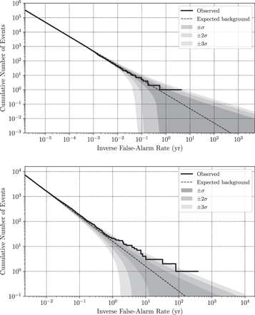
Figure 4. Combined results from the 39 subthreshold searches with the GstLAL pipeline (top panel) and PyCBC pipeline (bottom panel). Each panel shows, as a solid line, the cumulative number of coincident triggers (observed) with inverse FARs greater than or equal to a given value. The dashed line is the expected distribution of background triggers, with the gray bands indicating uncertainties in multiples of the standard deviation σ of a Poisson distribution. For GstLAL, the results for this plot are obtained by a search over all O3a data using a combined bank from the 39 targeted banks. For PyCBC, the FARs are from the individual searches, but for triggers found by several of the single-template searches, their inverse FARs have been summed.
Download figure:
Standard image High-resolution imageInstead, we perform follow-up analyses of the lensing hypothesis under the assumption of astrophysical origin, aiming to determine for each candidate pair in Table 4 whether it is more consistent with a pair of images of a single lensed event or with two independent astrophysical events. After taking into account the initial FAR thresholds, sky localization overlap, and data-quality checks, we have followed up six candidate pairs through LALInference joint Bayesian PE as described in Section 5.2.2. No special mitigation steps were required for data-quality reasons on any of the new candidates. The results are included in Table 4.
Compared with the results for the GWTC-2 pairs in Table 3, the LALInference coherence ratios alone are insufficient in providing evidence of lensing while keeping in mind selection effects and prior odds. As another cross-check, we have also analyzed the pair with the highest LALInference coherence ratio  (the candidate on 2019 September 16 found by the GW190620_030421 PyCBC search) with the hanabi pipeline described in Section 5.2.3. As with all previously tested pairs (see Table 3), after the inclusion of population priors and selection effects, there is no evidence favoring the lensing hypothesis for this pair either, with a population-weighted coherence ratio of
  and a Bayes factor of
 .
.
As lensing can produce more than two images of the same source, cases where several searches find the same trigger are of particular interest. We find that the same candidate on 2019 July 11 has been found with low FARs by three searches (targeting the GWTC-2 events GW190421_213856, GW190731_140936, and GW190909_114149). In addition, the trigger on 2019 August 5 is only found with a sufficient FAR for inclusion in Table 4 by a single GstLAL search (for GW190424_180648), but was also recovered by those for GW190413_052954 and GW190803_022701 with FARs just below the cut. However, the GWTC-2 pairs involved in these possible quadruple sets have already been significantly disfavored by the hanabi analysis including population priors and selection effects. We also expect such multiple matches from an unlensed BBH population due to the clustering of the GWTC-2 events in parameter space (Abbott et al. 2021a, 2021d).
Also, as discussed in detail in McIsaac et al. (2020), if any high-mass GW detections are interpreted as highly magnified images of lower-mass sources, then counterpart images for these would be more likely. However, we did not find any promising subthreshold candidates for the five events discussed under the lensing magnification hypothesis in Section 4.
In summary, the subthreshold searches can recover additional promising candidates that were not included in GWTC-2, which match other events closely and, in that sense, are consistent with the lensing hypothesis. However, we do not find sufficient evidence that they are indeed lensed images, as the set of results is also consistent with a population of physically independent and only coincidentally similar events.
6. Search for Microlensing Effects
Microlensing by smaller lenses produces image separations on the order of microarcseconds. For GWs, it can also induce frequency-dependent wave-optics effects similar to femtolensing of light (Nakamura 1998; Takahashi & Nakamura 2003). More specifically, when the characteristic wavelengths are comparable to the Schwarzschild radius of the lens, i.e.,  , it causes frequency-dependent magnification of the waveform. Moreover, the characteristic lensing time delay due to microlensed images can be shorter than the GW signal duration, causing potentially observable beating patterns on the waveform (Cao et al. 2014; Christian et al. 2018; Dai et al. 2018; Lai et al. 2018; Diego et al. 2019; Jung & Shin 2019; Diego 2020; Pagano et al. 2020; Cheung et al. 2021; Mishra et al. 2021), due to waveform superposition. To observe GW microlensing, we search for these beating patterns instead of the time-dependent change in the flux traditionally observed for microlensing in electromagnetic signals.
Here we search for microlensing by isolated point masses. The microlensed waveform has the form

where hML and hU are the microlensed and unlensed waveforms in the frequency domain, respectively. θ represents the set of parameters defining an unlensed GW signal, while  .
.  is the frequency-dependent lensing magnification factor, which is a function of the redshifted lens mass
  and dimensionless impact parameter y, given in Equation (2) of Lai et al. (2018). The search involves re-estimating the parameters of previously identified events under the microlensed hypothesis as defined in Equation (9), including those of the potential lens.
To measure the evidence of lensing signatures in a signal, we define a Bayes factor  , which is the evidence ratio between the microlensed and unlensed hypotheses. Higher positive values correspond to support for lensing. Hannuksela et al. (2019) searched for similar beating patterns due to point-mass lenses in the O1 and O2 data, using an upper lens mass prior cutoff of
  . They reported no evidence for such lensing patterns above
  .
.
For O3a, we analyze the 36 events from Abbott et al. (2021a) that confidently have both component masses above 3M⊙ and search for microlensing signatures following the same method as in Hannuksela et al. (2019). We perform PE using Bilby (Ashton et al. 2019; Romero-Shaw et al. 2020) and the nested sampling algorithm dynesty (Speagle 2020). For each event, we perform two PE runs using both unlensed and microlensed templates. For the unlensed case, which is similar to the usual PE analysis, equivalent prior settings and data dictionaries such as strain data and power spectral densities (PSDs) are used as in Abbott et al. (2021a). The analysis uses the IMRPhenomXPHM (Pratten et al. 2021) waveform for most events, except for GW190521, which is analyzed using the NRSur7dq4 waveform (Varma et al. 2019) and for the least massive event GW190924_021846 where the IMRPhenomPv2 waveform is used. The prior on  is log-uniform in the range [1–105
M⊙], above which the effect of microlensing is relatively small for the LIGO–Virgo sensitivity band. The impact parameter prior is p(y) ∝ y between [0.1, 3], chosen due to geometry and isotropy (Lai et al. 2018).
is log-uniform in the range [1–105
M⊙], above which the effect of microlensing is relatively small for the LIGO–Virgo sensitivity band. The impact parameter prior is p(y) ∝ y between [0.1, 3], chosen due to geometry and isotropy (Lai et al. 2018).
In Figure 5 we show violin plots of marginalized posterior distributions for the redshifted lens mass for each event, as well as the Bayes factors between the microlensed and unlensed hypotheses. The broad  posteriors correspond to broad posteriors on the impact parameter y, which is not well constrained for unlensed cases. In terms of Bayes factors, there is no substantial evidence of microlensing with a maximum
  for the event GW190910_112807. Additionally, as can be seen in Appendix C, statistical fluctuations of the log10 Bayes factors for injections without microlensing can be as high as 0.75. Thus, the observed Bayes factors are already by themselves consistent with random noise fluctuations and do not significantly favor the microlensing hypothesis for any of the events. The resulting posterior odds
  , which are the products of Bayes factors and the low prior odds of microlensing (Lai et al. 2018), would be even lower. Thus, we find no evidence of microlensing in this study.
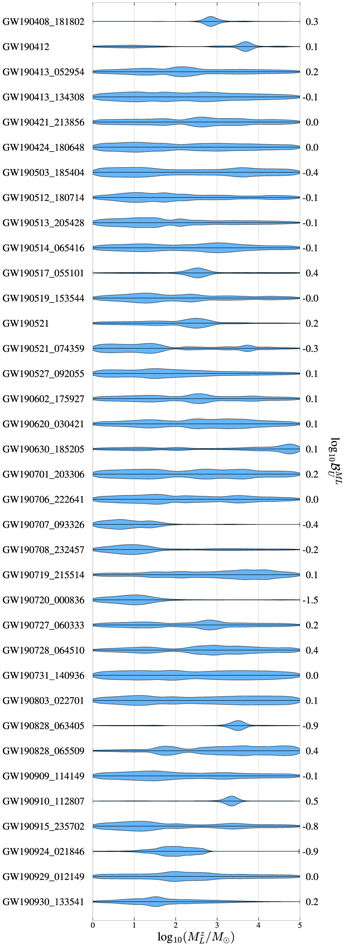
Figure 5. The marginalized posterior distribution of redshifted lens mass  and
and  between microlensed and unlensed hypotheses. The corresponding log10 Bayes factors are noted to the right of the plot. We find no evidence of microlensing by point-mass lenses.
Download figure:
Standard image High-resolution imageWe searched for microlensing due to isolated point masses. More complex models in which point-mass lenses embedded in an external macromodel potential such as galaxies and galaxy clusters (Diego et al. 2019; Cheung et al. 2021; Mishra et al. 2021) can produce additional modulation on the magnified waveform, which could also prove important in the LIGO–Virgo frequency band. Future searches could be extended to cover a broader range of microlensing models.
7. Conclusions and Outlook
We have searched for gravitational lensing effects on the GW observations from O3a, the first half of the third LIGO–Virgo observing run, finding no strong evidence of lensing. First, we outlined estimates for the rate of strongly lensed GWs. Second, presuming a non-observation of lensing, we constrained the BBH merger-rate density at high redshift. Third, we used merger-rate density models obtained through the non-observation of an SGWB to estimate the GW lensing rate.
Next, we performed an analysis of apparent high-mass events under the hypothesis that they are lensed signals from lower-mass sources, finding that the highest-mass BBHs from O3a could be consistent with component masses below the PISN mass gap, while GW190425 and GW190426_152155 would require extreme magnifications to be compatible with the Galactic BNS population. This hypothesis is at the moment mainly disfavored by the expected lensing rates, but in the future, more quantitative constraints could also be set by connecting these magnification results with lens modeling to make predictions for the appearance of multiple images or the possibility of microlensing.
We then searched for signatures of multiple lensed images from a single source through several methods. We first investigated the parameter consistency among all pairs of O3a events from GWTC-2 using a posterior-overlap method, finding no significant event pairs but identifying several interesting candidates with high overlap.
We followed up on these candidate pairs using two detailed joint-PE analyses, finding high parameter consistency for 11 pairs. However, after the inclusion of a more appropriate population prior, selection effects, and the prior odds against the lensing hypothesis, these candidates do not provide sufficient evidence for a strong lensing claim.
Moreover, we used two targeted matched-filter approaches to search for additional lensed images of the known events that could be hidden beneath the thresholds of the corresponding broader analyses used to produce GWTC-2, identifying six new candidates. After follow-up by joint PE, we found no evidence to conclude that any of these subthreshold triggers are lensed images.
Finally, we analyzed 36 events from GWTC-2 for microlensing effects by performing full PE with waveforms incorporating microlensing by point-mass lenses. We found no evidence of microlensing.
In summary, our results on the O3a data are consistent with the expected low rate of lensing at current detector sensitivities. However, improved analysis methods and lens modeling may allow one to digg deeper into potential lensing effects. Electromagnetic follow-up of lensing candidates, even if they are not significant enough based on the GW data alone, could also be promising (Sereno et al. 2011; Smith et al. 2018; Hannuksela et al. 2020; Yu et al. 2020). With the current generation of detectors further improving their sensitivity and the global network being extended (Abbott et al. 2020c), the chances of detecting clear lensing signatures will improve, and the field will offer many possibilities at the latest with third-generation (Punturo et al. 2010; Abbott et al. 2017; Reitze et al. 2019; Maggiore et al. 2020) and space-based detectors (Amaro-Seoane et al. 2017; Hu & Wu 2017) and their expected cosmological reach.
This material is based upon work supported by National Science Foundation's LIGO Laboratory, which is a major facility fully funded by the National Science Foundation. The authors also gratefully acknowledge the support of the Science and Technology Facilities Council (STFC) of the United Kingdom, the Max-Planck-Society (MPS), and the State of Niedersachsen/Germany for support of the construction of Advanced LIGO and construction and operation of the GEO600 detector. Additional support for Advanced LIGO was provided by the Australian Research Council. The authors gratefully acknowledge the Italian Istituto Nazionale di Fisica Nucleare (INFN), the French Centre National de la Recherche Scientifique (CNRS), and the Netherlands Organization for Scientific Research for the construction and operation of the Virgo detector and the creation and support of the European Gravitational Observatory (EGO) consortium. The authors also gratefully acknowledge research support from these agencies as well as by the Council of Scientific and Industrial Research of India; the Department of Science and Technology, India; the Science & Engineering Research Board (SERB), India; the Ministry of Human Resource Development, India; the Spanish Agencia Estatal de Investigación; the Vicepresidència i Conselleria d'Innovació Recerca i Turisme and the Conselleria d'Educació i Universitat del Govern de les Illes Balears; the Conselleria d'Innovació Universitats; Ciència i Societat Digital de la Generalitat Valenciana and the CERCA Programme Generalitat de Catalunya, Spain; the National Science Centre of Poland and the Foundation for Polish Science (FNP); the Swiss National Science Foundation (SNSF); the Russian Foundation for Basic Research; the Russian Science Foundation; the European Commission; the European Regional Development Funds (ERDF); the Royal Society; the Scottish Funding Council; the Scottish Universities Physics Alliance; the Hungarian Scientific Research Fund (OTKA); the French Lyon Institute of Origins (LIO); the Belgian Fonds de la Recherche Scientifique (FRS-FNRS); Actions de Recherche Concertées (ARC) and Fonds Wetenschappelijk Onderzoek—Vlaanderen (FWO), Belgium; the Paris Île-de-France Region; the National Research, Development and Innovation Office Hungary (NKFIH); the National Research Foundation of Korea; the Natural Science and Engineering Research Council Canada; Canadian Foundation for Innovation (CFI); the Brazilian Ministry of Science, Technology, and Innovations; the International Center for Theoretical Physics South American Institute for Fundamental Research (ICTP-SAIFR); the Research Grants Council of Hong Kong; the National Natural Science Foundation of China (NSFC); the Leverhulme Trust; the Research Corporation; the Ministry of Science and Technology (MOST), Taiwan; the United States Department of Energy; the Kavli Foundation; and the Gordon and Betty Moore Foundation. The authors gratefully acknowledge the support of the NSF, STFC, INFN, and CNRS for provisions of the computational resources.
We would like to thank all of the essential workers who put their health at risk during the COVID-19 pandemic, without whom we would not have been able to complete this work.
Software: Analyses in this paper made use of LALSuite (LIGO Scientific Collaboration & Virgo Collaboration 2018), the GstLAL (Cannon et al. 2012; Messick et al. 2017; Sachdev et al.2019; Hanna et al. 2020) and PyCBC (Usman et al. 2016; Nitz et al. 2018, 2019; Davies et al. 2020) pipelines; Bayesian inference with CPNest (Veitch et al. 2020), PyMultinest (Feroz et al. 2009, 2019), Bilby (Ashton et al. 2019; Romero-Shaw et al. 2020; Smith et al. 2020), and LALInference (Veitch et al. 2015); as well as the packages NumPy (Harris et al. 2020), SciPy (Virtanen et al. 2020), Astropy (Robitaille et al. 2013; Price-Whelan et al. 2018), IPython (Perez & Granger 2007), and ligo.skymap (Singer 2019). Plots were produced with Matplotlib (Hunter 2007), and Seaborn (Waskom et al. 2020).
Appendix A: Supplementary Lensing Statistics
Assuming a specific BBH formation channel, we can estimate the lensing rate for merger signals from that population. For example, suppose BBHs form as a consequence of isolated binary evolution. In that case, one can theoretically model BBH formation assuming that it traces the star formation rate, modulated by the delay-time distribution and by the stellar metallicity evolution (Belczynski et al. 2008, 2010; Dominik et al. 2013; Marchant et al. 2018; Boco et al. 2019; Eldridge et al. 2019; Neijssel et al. 2019; Santoliquido et al. 2021). However, note that if the BBHs form through other means or through multiple channels, the merger-rate density could be different (e.g., Miller & Lauburg 2009; Antonini & Rasio 2016; Rodriguez & Loeb 2018; Antonini & Gieles 2020; De Luca et al.2020; Fragione & Silk 2020; Bouffanais et al. 2021; Wong et al. 2021; Zevin et al. 2021).
Here we assume two models for the merger-rate density. We base the first model on the assumption that the merger-rate density of the observed BBHs traces the star formation rate density and that the BBHs originate from Population I/II stars.
In this work, we did not consider the contribution of Population III stars. Population III stars have not been observed yet, and their physical properties, binary fraction, and initial mass function are still a matter of debate (Madau & Rees 2001; Nakamura & Umemura 2001; Bromm et al. 2002; Schaerer 2002; Machida 2008; Norman 2008; Ishigaki et al. 2018). As such, the contribution of Population III BBHs to GW sources is also uncertain (e.g., Bond & Carr 1984; Kowalska et al. 2012; Belczynski et al. 2017; Liu & Bromm 2020). Should Population III stars dominate the BBH formation at high redshift, our results would need to be reinterpreted.
The first model, which we label Model A, uses the following fits which bracket the available population synthesis results from the literature (e.g., Belczynski et al. 2008, 2010; Dominik et al. 2013; Marchant et al. 2018; Boco et al. 2019; Eldridge et al. 2019; Neijssel et al. 2019; Santoliquido et al. 2021):
where the fitting parameters a1 = 58.497, a2 = 2.06424, a3 =2.82338, a4 = 2.52898, b1 = 105356, b2 = 1.30278, b3 =2714.36, and b4 = 2.22903.
We base the second model, Model B, on the assumption that the merger-rate density follows the Madau & Dickinson (2014) ansatz:
To constrain the merger-rate density at high redshift, we assume that no strong lensing has occurred (Section 3.2). We further assume that events occur following a Poisson process.
Let us now assume Model B for the merger-rate density, Equation (A2). The distribution of the merger-rate density parameters, given that no strong lensing has occurred, is

where p(R0, κ, γ, zp ∣{di }) follows the posterior distribution of parameters inferred from LIGO–Virgo population studies (Abbott et al. 2021d), and
with N being the number of observed, strongly lensed GW signals, and Navg(R0, κ, γ, zp
) is the expected number of events within a time Δt. Here, like in Section 3, we do not account for detector downtime, and instead as a proxy presume that the detectors are always online. The R0 and κ values are measured at a low redshift (Abbott et al. 2021d). The γ and zp
values are unconstrained here and thus match an uninformative prior, with  being a split normal distribution and p(zp
) being uniformly distributed between [0, 4]. The above equations give all the necessary ingredients to forecast the rate of strongly lensed events and place constraints on the merger-rate density based on the number of lensed signals observed by LIGO and Virgo.
being a split normal distribution and p(zp
) being uniformly distributed between [0, 4]. The above equations give all the necessary ingredients to forecast the rate of strongly lensed events and place constraints on the merger-rate density based on the number of lensed signals observed by LIGO and Virgo.
Appendix B: Construction of Subthreshold Counterpart Search Template Banks
For the GstLAL and PyCBC searches for subthreshold lensed counterparts (Section 5.3) the targeted template banks for each event are constructed starting from a certain choice of posterior distributions released with GWTC-2 (GWOSC 2020; Abbott et al.2021a), aiming for a reduced-size template bank that is effective at recovering signals similar to the primary observed event.
For the GstLAL pipeline, we start, for all but three of the O3a events from GWTC-2, from nonspinning posteriors obtained with the IMRPhenomD waveform (Husa et al. 2016; Khan et al. 2016). In three cases, we instead start from posteriors obtained with the IMRPhenomPv2 waveform (Hannam et al. 2014; Bohé et al. 2016), which includes spin precession. These exceptions are GW190413_052954, GW190426_152155, and GW190909_114149. We then choose subsets of the original broad template bank from the GWTC-2 analysis by comparing against the posteriors of each event, using the following steps as introduced by Li et al. (2019a): we first draw O(1000) of each event's posterior samples with the highest likelihoods to account for the uncertainty in the event's measured mass and spin parameters. For each sample we simulate, using the aligned-spin SEOBNRv4_ROM waveform model (Pürrer 2014, 2016; Bohé et al. 2017), one signal with the event's original optimal S/N ρopt as given by Equation (2) in Li et al. (2019a) and nine extra signals with smaller ρopt, scaled by changing their effective distances Deff (Allen et al. 2012). The reduced template bank for an event is then constructed by searching the simulated data with the original GWTC-2 template bank (which also consists of SEOBNRv4_ROM waveforms) and keeping those templates which recover any of the simulated signals with an FAR < 1 in 30 days.
For PyCBC we select a single template for each search, choosing the maximum-posterior redshifted masses and aligned-spin components {(1 + z)m1, (1 + z)m2, χ1, χ2} as estimated from a four-dimensional Gaussian KDE fit to the posterior samples from GWOSC (2020) for these parameters. Where available, we use aligned-spin posterior samples. In the case of GW190412 and GW190814, we use samples generated using the SEOBNRv4_ROM waveform; for GW190426_152155 we use a mixture of samples generated using the SEOBNRv4_ROM_NRTidalv2_NSBH and IMRPhenomNSBH waveforms; and for GW190425 we use samples generated using the IMRPhenomD_NRTidal, TEOBResumS, and SEOBNRv4T_surrogate waveforms. If aligned-spin posteriors are not available in the GWOSC (2020) data release, we use precessing posterior samples and marginalize over the transverse-spin components before applying the KDE. This produces an aligned-spin template with high matches at the peak of the posterior. In the case of GW190521, we use samples generated using the IMRPhenomPv3HM (Khan et al. 2020), NRSur7dq4 (Varma et al. 2019), and SEOBNRv4PHM (Ossokine et al. 2020) waveforms. For all other events, we use samples generated using the SEOBNRv4P and IMRPhenomPv2 waveforms.
These choices of waveforms and posterior samples are not necessarily optimal, but they are valid for this analysis in the sense that the recovery of similar waveforms with parameters close to the best-fit ones for the targeted GWTC-2 events has been verified through injection studies. In addition, in the actual searches, the targeted banks constructed in this way successfully recovered the corresponding GWTC-2 events in all GstLAL searches, while for PyCBC triggers within 0.1 s of the target events were excluded from the final trigger list, but in all cases where the original events were observed with two or more detectors, a coincident trigger was also recovered in the targeted search. In future work, revisiting the choice of posterior samples used to construct template banks may further improve the effectiveness of subthreshold searches.
Appendix C: Injection Study for Microlensing Analysis
A high Bayes factor  itself is not conclusive evidence of microlensing in an observed event. We have performed an injection study to explore the impact of statistical fluctuations on the Bayes factor obtained from unlensed signals. We generate unlensed injections by randomly drawing from the parameter space of precessing BBH systems. Simulated Gaussian noise is used considering nominal O3 sensitivity (Abbott et al. 2020c), and we use the IMRPhenomPv2 waveform model (Hannam et al. 2014; Bohé et al. 2016) for all simulated injections. The statistical fluctuations of
  for 100 unlensed injections recovered using lensed templates can been seen in Figure 6 which shows that the typical values found are
  .
.
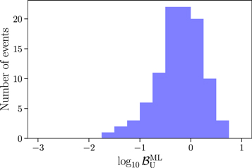
Figure 6. Distribution of microlensing Bayes factors  for unlensed simulated signals, recovered using a lensed template.
Download figure:
Standard image High-resolution image