


Abstract
We present a two-dimensional radiative-dynamical model of the combined stratosphere and upper troposphere of Jupiter to understand its temperature distribution and meridional circulation pattern. Our study highlights the importance of radiative and mechanical forcing for driving the middle atmospheric circulation on Jupiter. Our model adopts a state-of-the-art radiative transfer scheme with recent observations of Jovian gas abundances and haze distribution. Assuming local radiative equilibrium, latitudinal variation of hydrocarbon abundances is not able to explain the observed latitudinal temperature variations in the mid-latitudes. With mechanical forcing parameterized as a frictional drag on zonal wind, our model produces ∼2 K latitudinal temperature variations observed in low to mid-latitudes in the troposphere and lower stratosphere, but cannot reproduce the observed 5 K temperature variations in the middle stratosphere. In the high latitudes, temperature and meridional circulation depend strongly on polar haze radiation. The simulated residual mean circulation shows either two broad equator-to-pole cells or multi-cell patterns, depending on the frictional drag timescale and polar haze properties. A more realistic wave parameterization and a better observational characterization of haze distribution and optical properties are needed to better understand latitudinal temperature distributions and circulation patterns in the middle atmosphere of Jupiter.
Export citation and abstract BibTeX RIS
1. Introduction
Jupiter's upper troposphere and stratosphere are home to a host of unexplained dynamical processes. From distributions of radiatively active trace gases concentrated far from their source region (Nixon et al. 2010; Zhang et al. 2013a) to wave structures and local disturbances in observed temperature distributions (Leovy et al. 1991; Simon-Miller et al. 2007; Cosentino et al. 2017) to the unknown relationship between convection processes in the troposphere and their generated wave interactions with the layers above (Ingersoll et al. 2004; Fletcher et al. 2020), there is ample reason to better understand the mean flow and circulation dynamics occurring in the Jovian middle atmosphere.
Latitudinal variations in temperature provide insights into the radiative and dynamical processes of the middle atmosphere. At low latitudes, a semi-periodic oscillation in equatorial and off-equatorial brightness temperatures has been observed in Jupiter's stratosphere since the 1980s. Called the Quasi-Quadrennial Oscillation (QQO), it has been compared to Earth's own Quasi-Biennial Oscillation (QBO), a layering of east–west stratospheric jets produced by wave forcing (Orton et al. 1991; Leovy et al. 1991; Friedson 1999; Simon-Miller et al. 2007; Cosentino et al. 2017, 2020). At high latitudes, temperatures can rise nearing the poles due to extended layers of stratospheric haze spanning ∼1–250 mbar. Quantifying the radiative effect of haze layers is essential to explain the observed temperature at the poles (Guerlet et al. 2020). To date, the vertical extent, meridional distribution, and optical properties of Jovian haze are still not well constrained (Kedziora-Chudczer & Bailey 2011; Zhang et al. 2013b, 2015). In the mid-latitudes, temperatures at a given pressure level can vary latitudinally by up to 5–10 K from the global mean. It is still unclear whether radiation or dynamics is the driving force behind this variation. Supporting the radiative argument, observed C2H2, C2H6, and haze particles are not well mixed throughout the middle atmosphere and should influence localized variations in net heating (Moses et al. 2005; Nixon et al. 2010; Zhang et al. 2013a; Fletcher et al. 2016a). Dynamics, however, could perturb the middle atmosphere due to a variety of wave activities (Conrath et al. 1990).
It is not easy to quantify the effect of dynamics in the middle atmosphere because the stratospheric wind pattern has not been directly observed. Measurements of zonal wind speed are limited to the visible cloud layers below the tropopause (Atkinson et al. 1996; Porco et al. 2003). Instead, retrievals of zonally averaged temperature provide the only window into stratospheric flow. Latitudinal temperature variations are associated with vertical shear in the zonal wind via thermal wind balance (Andrews et al. 1987). Several studies have calculated the wind distribution from observed temperatures (e.g., Flasar et al. 2004; Simon-Miller et al. 2006; Fletcher et al. 2016a). These studies show jets at the cloud level extending up to 1 mbar and seem to imply strong oscillations with height near the equator. Fletcher et al. (2016b) used a Monte Carlo approach to demonstrate that uncertainties in this calculation reach ∼10 m s−1 at mid-latitudes near 100 mbar and climb to hundreds of m s−1 in the equatorial stratosphere. Thus, we primarily understand only the qualitative features of the zonal wind pattern in Jupiter's stratosphere.
Meridional circulation ("residual mean circulation") in Jupiter's middle atmosphere can also be derived from the observed zonal-mean temperature distribution (West et al. 1992; Moreno & Sedano 1997; Guerlet et al. 2020). This method (hereafter, the "post-analysis" method) calculates the balance between radiative heating and adiabatic cooling/heating associated with vertical transport by assuming that the eddy heat flux convergence is negligible, which is a typical approximation for large-scale quasi-geostrophic flows outside of acceleration conditions (Andrews et al. 1987; West et al. 1992). This method was pioneered on Jupiter by West et al. (1992), who included approximations of stratospheric haze heating neglected by Conrath et al. (1990), and was revisited in subsequent studies (Moreno & Sedano 1997; Guerlet et al. 2020).
However, "first-principles" calculations of circulation patterns in the middle atmosphere require a detailed treatment of the interaction between radiative and dynamical processes. Although a three-dimensional (3D) general circulation model (GCM) can self-consistently capture wave-mean interactions, it is computationally expensive to run over timescales relevant for giant planets. Therefore, it is difficult for this approach to explore the entire parameter regime. To date, global 3D GCMs of Jupiter focus mainly on the tropospheric processes rather than the stratosphere (Lian & Showman 2008; Schneider & Liu 2009; Lian & Showman 2010; Liu & Schneider 2010, 2011; Young et al. 2019a, 2019b). Stratospheric GCMs have only been implemented for Saturn (Friedson & Moses 2012; Spiga et al. 2020). Conversely, a two-dimensional (2D) zonal-mean circulation model in latitude-pressure coordinates has a simplified setup and can be easily applied to a large parameter space. It is also computationally affordable and can incorporate necessary interactive processes, including radiation, dynamics, and chemistry, in a single framework to investigate the large-scale features in the middle atmospheres of giant planets.
Two-dimensional models with the linearized form of the equations of motion have been previously used to study Jupiter's middle atmosphere. Gierasch et al. (1986) used temperature observations from the Voyager spacecraft to calculate meridional circulation at selected pressure levels. A more comprehensive survey by Conrath et al. (1990) examined middle atmosphere circulation on the four solar system gas planets by using a simple Newtonian cooling radiative scheme and a linear frictional drag on zonal wind. Cosentino et al. (2017, 2020) explored the parameterization of gravity wave drag in a 2D circulation model to induce a QQO-like temperature structure near the equator, also using a Newtonian cooling scheme, but did not examine circulation on a global scale. The main problem with Conrath's model is that the calculated radiative timescale in Jupiter's atmosphere, which increases from ∼1500 days at 1000 mbar to ∼3400 days at 0.01 mbar, is not accurate. With the recently observed hydrocarbons and hazes that have been significantly improved since Conrath et al. (1990), the latest radiative transfer calculations find that the radiative timescale in the Jovian atmosphere is ∼1700 days between 1000 and 50 mbar, then gradually decreases to ∼50–100 days by 0.01 mbar (Zhang et al. 2013a; Kuroda et al. 2014; Li et al. 2018a; Guerlet et al. 2020).
Instead of using a Newtonian cooling scheme, in this study we develop a 2D circulation model using more accurate radiative transfer informed by the Voyager and Cassini flybys of Jupiter and recent ground-based observations to better understand the mechanisms behind meridional circulation in the Jovian stratosphere and upper troposphere. We describe the model's structure and the methods used to perform calculations of radiative forcing and dynamics in Section 2. In Section 3 we present results from simulations of Jupiter's middle atmosphere and compare those with observations of temperature. In Section 4 we discuss the study's implications for future observation campaigns and the next steps of circulation modeling.
2. Jupiter 2D Radiative-dynamical Model
2.1. Radiative Transfer
2.1.1. Correlated-k Two-stream Radiative Transfer Solver
Solar heating in Jupiter's atmosphere in UV, visible, and near-infrared bands is primarily dominated by CH4 and hazes while infrared (IR) cooling is controlled by CH4, C2H2, C2H6, NH3, PH3, collision-induced absorptions (CIAs) of H2–H2 and H2–He, as well as haze opacities in the mid-infrared (Zhang et al. 2015). In our radiative transfer model, we consider the wavelength range from 0.2 to 100 microns. The gas opacity is calculated using the "HARP" model that is thoroughly discussed and validated in Li et al. (2018a). Molecular absorption lines are mainly from the HITRAN 2016 database (Gordon et al. 2017) but we use hydrogen-broadening line widths for C2H2 and C2H6 (Zhang et al.2013a; Li et al. 2018a). The opacity data of H2–H2 and H2–He CIA are obtained from Orton et al. (2007). Since the spectroscopic line list of CH4 in HITRAN 2016 is incomplete beyond 7900 cm−1, we additionally use an ab initio line list to fill in missing transitions throughout the spectrum and add CH4 lines from 7900 cm−1 to 12,000 cm−1 (Rey et al. 2016). The full details of this addition and its influence on heating rates are explained in Guerlet et al. (2020), but the ultimate effect is a slightly increased globally averaged temperature (2–3.5 K) which has a maximum change near 10–20 mbar.
In the infrared bands, correlated-k absorption coefficients are calculated from line-by-line opacities generated with a spectral resolution of 0.1 cm−1 (Gordon et al. 2017). To ensure accuracy, we adopt 17 infrared bands defined in Kuroda et al. (2014) corresponding to the vibrational–rotational bands of CH4, C2H2, and C2H6. Sixteen Gaussian quadrature points were used for each band interval to calculate the correlated-k coefficients. Agreement of the thermal cooling rates between correlated-k and line-by-line flux calculations is well within 10% (Li et al. 2018a) and the difference in radiative equilibrium temperature between the two methods is smaller than 1% in Jupiter's stratosphere. The correlated-k method allows for much faster computation times than line-by-line, which is too slow for use in 2D and 3D models of giant planets that often require simulating tens to hundreds of years before achieving steady state.
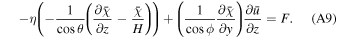
Gas abundance and initial temperature are taken from Zhang et al. (2013a). In our model, the hydrocarbon abundances are assumed to be uniform with latitude. The vertical profiles of C2H2 and C2H6 are plotted in Figure A1. If we use the globally averaged hydrocarbon profiles from Zhang et al. (2013a), the simulated global average temperature in the upper stratosphere is ∼5 K below observed values at pressures <3 mbar, confirming a similar result from Guerlet et al. (2020). The net cooling rates in Jupiter's mid- to upper stratosphere are primarily influenced by C2H2 and C2H6, particularly in the pressure levels between 0.002 and 1 mbar (Zhang et al. 2013a). To explain the observed temperature, we reduce C2H2 and C2H6 abundances by 50% uniformly, and above 0.3 mbar further by (p/0.3 mbar)0.4. This adjustment is ad hoc and chosen to approximate the observed mean temperature in the upper stratosphere, but it still falls within uncertainty in the hydrocarbon abundance retrieval by Zhang et al. (2013b). In particular, current gas abundance measurements are fairly unreliable above 0.1 mbar.
Radiative transfer equations including multiple scattering are solved with a two-stream approximation (Kylling et al. 1995). A similar numerical implementation has been applied to GCMs of exoplanets and brown dwarfs (Komacek et al. 2017; Tan & Showman 2021). An internal heat flux of 7.48 W m−2 (Li et al. 2018b) is also added as a radiative flux at the bottom of our model. To reduce the computational cost, we only update the radiative transfer calculations once per Earth day, which is sufficient to produce accurate results. Because we wish to examine the ability of the model to reproduce Jupiter's temperature distribution and circulation in steady-state conditions, we exclude seasonal variations due to Jupiter's small obliquity (3.13°) and orbital eccentricity (0.048). Diurnal variations are also neglected because of Jupiter's fast rotation: Guerlet et al. (2020) determined that the maximum amplitude of diurnal temperature variations is less than 0.1 K.
2.1.2. Haze and Cloud Properties
We include both stratosphere and upper troposphere hazes in the radiative transfer calculation. Haze solar heating is calculated with the haze optical properties of Guerlet et al. (2020) scenario #2, which were derived from Zhang et al. (2013b). The infrared cooling rate of the haze is calculated based on Zhang et al. (2015). Tropospheric haze and clouds are modeled in the same method as the nominal model presented in Guerlet et al. (2020): a haze layer with an integrated optical depth of 4 in the range 660–150 mbar, "gray" particles of radius 0.5 μm on top of an NH3 cloud (or indifferently a "gray" cloud) with 10 μm particles, and a cloud deck at 840 mbar with an integrated optical depth of 15 at 750 nm. Discussion of the sensitivity tests performed on these parameters can be found in that study. Note that the spatial distribution and opacities of the polar stratospheric haze have large uncertainties. In Zhang et al. (2013b), the haze spatial distribution is retrieved from near-IR data between −75°S and 25°N. Northward of 25°N, the shape of the distribution is assumed to be the same as the southern hemisphere. The UV and visible opacities of the haze are constrained by Cassini image data. The mid-infrared opacities of the haze are estimated in Zhang et al. (2015) to ensure globally averaged heating and cooling balance. A separate set of observations with the Anglo-Australian Telescope, however, found a slightly different haze distribution, with two distinct layers of polar haze at ∼2–7 mbar and ∼25–250 mbar, though the vertical extents of the north and south polar distributions were not the same (Kedziora-Chudczer & Bailey 2011). The haze distribution used in our model is plotted in Figure A1.
2.2. SOCRATES 2D Dynamical Model
We use a 2D dynamical prescription formulated in transformed Eulerian mean (TEM) coordinates (Andrews & McIntyre 1976; Boyd 1976). This model originated at the National Center for Atmospheric Research as SOCRATES (Simulation of Chemistry, Radiation, and Transport of Environmentally important Species) and has been used to model dynamics, radiation, and chemistry in the middle atmosphere of Earth (e.g., Brasseur et al. 1990; Huang et al. 1998). We adapt the dynamical core for use with Jupiter, solving the zonally averaged quasi-geostrophic equations:


Here, z represents log-pressure altitude defined as  , ps is base-of-model ("surface") pressure, H is a fixed scale height (set at 27 km for Jupiter), ϕ is latitude,
  is zonal-mean potential temperature,
  is zonal-mean zonal wind, a is planetary radius, y is a
ϕ, Ω is planetary rotation rate, atmospheric density
is zonal-mean zonal wind, a is planetary radius, y is a
ϕ, Ω is planetary rotation rate, atmospheric density  , the Coriolis parameter
  , and the dry specific gas constant for Jupiter's hydrogen–helium atmosphere R ≈ 3615 Jk−1gK−1. Thermodynamical forcing in Equation (1) includes the net diabatic heating rate (Q) and small-scale diffusive transport of heat by eddy and molecular diffusion processes:
where Kyy
is the meridional eddy diffusivity coefficient, Kzz
is the vertical eddy diffusivity coefficient, and KT
is the molecular thermal conductivity coefficient. Temperature and density fields are advected by  and
and  , the meridional and vertical components of residual mean circulation.


The derivation of the combined equations into an equation of volume stream function χ can be found in the Appendix, verifying the solution of Garcia & Solomon (1983). The solver eliminates time derivatives and iterates the system until a true steady state is reached (see Huang et al. 1998).
Forcing F in Equation (2) can be any physical source of momentum deposition, mainly caused by planetary/gravity wave dissipation and/or breaking. However, in this study we will only use a drag force  with timescale τf
to represent forcing that opposes the zonal-mean flow (Conrath et al. 1990). Kzz
in the upper troposphere is not well known. We found that linearly relaxing in log-pressure space from 20 m2 s−1 at 3000 mbar to 0 at the 100 mbar tropopause resulted in the best fit for globally averaged temperature below the tropopause (see the profile in Figure A1). This roughly estimates vertical diffusion as Kzz
≃ wH (Zhang & Showman 2018a, 2018b) if vertical eddy motion within the upper troposphere is approximately 0.1–1 mm s−1. For simplicity, we set KT
to a negligibly small value and Kyy
= 0.
with timescale τf
to represent forcing that opposes the zonal-mean flow (Conrath et al. 1990). Kzz
in the upper troposphere is not well known. We found that linearly relaxing in log-pressure space from 20 m2 s−1 at 3000 mbar to 0 at the 100 mbar tropopause resulted in the best fit for globally averaged temperature below the tropopause (see the profile in Figure A1). This roughly estimates vertical diffusion as Kzz
≃ wH (Zhang & Showman 2018a, 2018b) if vertical eddy motion within the upper troposphere is approximately 0.1–1 mm s−1. For simplicity, we set KT
to a negligibly small value and Kyy
= 0.
The model is sensitive to the boundary conditions of both zonal-mean zonal wind and the stream function. At the top of the model we have a "sponge layer" where  ,
,  , and χ are damped to zero. In the bottom layer, zonal wind
  is fixed to the observed zonal wind from cloud tracking by the Cassini Imaging Science Subsystem (ISS; Porco et al. 2003). This is similar to the setup of Conrath et al. (1990)'s "mechanically forced" models, which used wind speeds from Voyager. For the lower boundary condition of the stream function, the "downward control principle" states that mass flow across an isentropic surface is controlled by the amount of eddy forcing above that surface (Haynes et al. 1991; Garcia et al. 1992). From a linearized, steady-state momentum equation,
  , Equation (6) allows us to estimate at the lower boundary as:

A simplification of the solution is possible based on an order of magnitude estimate of F on the lower boundary, Fb = − ub /τf :

We tested Equations (8) and (9) as bottom boundary conditions in our model and both produced nearly identical results. Equation (8) is adopted as the boundary condition for results presented in this paper. Conrath et al. (1990) derived a similar estimate of circulation at the lower boundary of their model (Equation (29)). However, their equation is erroneous in that a zonal wind pattern u that is symmetric about the equator would result in an asymmetric vertical wind pattern w, which is physically incorrect.
We use a 141 cell latitude grid, 61 layer pressure grid from 0.003 to 3000 mbar, evenly distributed in log-pressure space. Our quasi-geostrophic assumption breaks down very close to the equator where the Coriolis parameter f approaches 0. In particular, we did not solve the thermal wind equation (Equation (4)) within ±10° of the equator. Instead, we linearly interpolated the wind solution across that region. For the sake of accuracy, we do not consider results within ±10° of the equator throughout this study (Huang et al. 1998). A standard Shapiro filter was used to control noise at the grid scale. We use a dynamical timestep of one Earth day. Models are run to 12 Jovian years, with steady state usually achieved within 2–5 Jovian years.
3. Results and Comparison to Observations
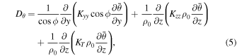
Observations of spatial and temporal distributions of Jovian atmospheric temperature were retrieved from spectra obtained by the Infrared Interferometer Spectrometer and Radiometer (IRIS) onboard Voyager and the Composite Infrared Spectrometer (CIRS) onboard Cassini during Jupiter flybys (Simon-Miller et al. 2006; Nixon et al. 2010; Zhang et al. 2013a). Earth-based observations continue to the present, most notably from telescopes at NASA's Infrared Telescope Facility (IRTF) using the Texas Echelon Cross Echelle Spectrograph (TEXES) instrument (Lacy et al. 2002; Fletcher et al. 2016a; Sinclair et al. 2017b; Melin et al. 2018). We compare our results with retrievals by Zhang et al. (2013a) of the Voyager IRIS data from 1979, and by Fletcher et al. (2016a) of the Cassini CIRS data from 2000 and TEXES data from 2014. We interpolate the observed temperature data to the model pressure grid to compare with our model results.
3.1. Radiative Equilibrium
We first examine the radiative model without dynamics, resulting in a radiative equilibrium (RE) temperature distribution. The global mean temperature profiles for IRIS, CIRS, and TEXES observations between 78°S and 78°N are shown in Figure 1. Temperatures between 10°S and 10°N are excluded because of model inaccuracy near the equator, but including them does not noticeably change the results. Our nominal RE model is able to reproduce observations above the tropopause at around 100 mbar. In the region near and below the tropopause, temperature is not expected to be in radiative equilibrium due to convection in the troposphere. Instead, the vertical temperature profiles should essentially follow the adiabat. We will discuss the dynamical circulation model in Section 3.2.

Figure 1. (a) Globally averaged temperature profiles from observations by IRIS (Zhang et al. 2013a), CIRS, and TEXES (Fletcher et al. 2016a) (symbols) and model predictions (colored lines), between ±78°, excluding values from the tropical region within ±10° where our geostrophic model lacks accuracy. The RE model is a radiative equilibrium model defined in Section 3.1, and the dynamical model (labeled as "Dyn 200d") has frictional drag throughout the atmosphere with a 200 day drag timescale, described in Section 3.2. (b) Globally averaged radiative timescale τr , and drag timescale τf used in two dynamical models found in Section 3.2.
Download figure:
Standard image High-resolution imageLatitudinal distributions of the stratospheric temperature at specific pressure levels are presented in Figure 2. Observations were obtained at different times of the Jupiter year: IRIS in 1979, northern autumnal equinox, CIRS in 2000, early northern summer, and TEXES in 2014, late northern summer. Jupiter's zonally averaged temperature distribution changes significantly over time, but all observations show latitudinal variations throughout the middle atmosphere. The strong temperature variability near the equator in CIRS and TEXES observations, associated with a QQO that is believed to be a result of wave-mean flow interaction similar to stratospheric QBO on Earth (Orton et al. 1991; Cosentino et al. 2017, 2020) cannot be explained by our RE model without dynamics. Also, our 2D model assumes quasi-geostrophic motion and thus lacks accuracy near the equator (see Section 2.2). Therefore, we will not discuss equatorial temperature variations in this study.

Figure 2. Comparison of observed stratospheric temperatures from IRIS (Zhang et al. 2013a), CIRS, and TEXES (Fletcher et al. 2016a) (symbols), and predictions by the radiative equilibrium (RE) model (lines), at four different pressures. The RE model is a radiative equilibrium model described in Section 3.1, and HC ±20% represents an increase/decrease in C2H2 and C2H6 mixing ratios. The gray band represents the equatorial zone where our model lacks accuracy.
Download figure:
Standard image High-resolution imageThe RE model produces temperature distributions that reside between the general trends of IRIS, CIRS, and TEXES observations in most of the stratosphere (Figure 2). We only compare the RE model with the data at several stratospheric levels as only the stratosphere might be assumed in radiative equilibrium. The match of temperature at these levels is comparably similar to the RE model study in Guerlet et al. (2020). The general trend from low to mid-latitudes basically follows solar insolation, which is maximal approaching the equator. At high latitudes, polar hazes influence the temperature via solar energy absorption and infrared cooling. Observations show that temperatures around 7 and 30 mbar increase from the mid-latitude to about ±60° latitude and then drop toward the poles. At lower pressure (above 3 mbar), the polar temperature decreases less rapidly and even increases toward the pole in the CIRS data at around 0.5 mbar. Our model is able to qualitatively reproduce this general trend due to the effect of polar haze (see Guerlet et al. 2020 for more discussion), including the temperature peak near the sub-polar region. However, the simulated temperature at ∼30 mbar begins decreasing at a lower latitude (±50°), as opposed to observational decreases closer to ±60–70°. At 3 mbar, our model overpredicts temperatures at the poles, where the influence of haze heating is strongest. Our model could also not explain the hot poles at 0.5 mbar in the CIRS data. However, note that there is a large variation between the CIRS data and TEXES data in the polar region. This suggests that the polar region in Jupiter's stratosphere is very dynamic and the temperature varies significantly with time, perhaps due to some additional heating mechanism such as the precipitation of the high-energy particles in the polar auroral region (Friedson et al. 2002; Mauk et al. 2017). The mismatch between our model and the observations could also originate from uncertainties in the spatial distribution of the haze layer and the haze optical properties used in our model, which are not well constrained (see Section 2.1.2). Future characterizations of the stratospheric haze with higher accuracy will allow for a better fit to observed polar temperatures in the mid- to lower stratosphere.

Figure 3. Comparison of observed stratospheric temperatures from IRIS (Zhang et al. 2013a), CIRS, and TEXES (Fletcher et al. 2016a) (symbols), and predictions by the radiative equilibrium (RE) model,the dynamical model with a uniform drag timescale τf = 200 days, and dynamical models with τf that decreases linearly with altitude from the bottom of the model to the top (200 days to 10 days, and 2000 days to 100 days). The gray band represents the equatorial zone where our model lacks accuracy.
Download figure:
Standard image High-resolution imageOur RE model does not show strong variations of ±5 K in the mid-latitudes. Although the model uses a uniform global average for gas abundances, introducing the observed variations of gases cannot explain the temperature contrast. Between 0.03–2 mbar, the latitudinal contrast of the strongest coolant, C2H6, is around 10%–20% in the low and mid-latitudes (see Figure 3 in Zhang et al. 2013a). By changing the latitudinally uniform C2H6 abundance by 20% in the model ("HC ± 20%" in Figure 2), we show that the temperature can at most change by ∼2 K. This indicates that even if we impose a latitudinal variation of the hydrocarbon abundances by up to 20% in our model, we do not expect that it would resolve the mismatch between our RE results and the observations. A plausible explanation for the latitudinal variation of temperature is atmospheric dynamics, as we will discuss below.
In the polar region, the hydrocarbon abundance could vary much more than 20% due to auroral-related chemistry (Sinclair et al. 2017a, 2018, 2019). However, thick haze layers might contribute much more to the radiative heating than the gases in the polar region (Zhang et al. 2015; Sinclair et al. 2017a; Guerlet et al.2020). Therefore, the temperature variations might be related to a combination of local haze variability and active auroral-related processes such as precipitation of high-energy particles. Furthermore, a possible origin of the variability due to upward propagating waves from the troposphere cannot be excluded as Jupiter's polar troposphere is strongly shaped by multiple large cyclones (Adriani et al. 2018). The stratospheric temperature distribution in the polar region needs a special investigation in the future and will not be focused upon in this study.
3.2. Dynamical Simulation Results
Here we present fully coupled 2D radiative-dynamical model results. From thermal wind balance, observed meridional temperature gradients in Jupiter's upper troposphere indicate that zonal winds decay with altitude, perhaps due to deceleration by eddy forces (Conrath et al. 1990; Fletcher et al. 2020). Residual meridional circulation is required to balance eddy forces on zonal jets under a quasi-geostrophic condition (Holton 2004; Fletcher et al. 2020). Those eddies likely originate from convectively generated waves in the troposphere, but their subsequent upward propagation and interaction with the mean flow in the overlying stratosphere is not well understood (Showman et al. 2019; Fletcher et al. 2020). Important wave generation and propagation processes may occur in a scale currently too small for a 3D GCM (Cosentino et al. 2017, 2020). Our 2D model lacks the ability to self-consistently produce waves, so mechanical forcing must be prescribed and parameterized.
Rayleigh friction, represented as a linear drag force opposing zonal-mean flow, has long been used as the simplest parameterization for the mean effect of complex atmospheric interactions (Gierasch et al. 1986). Conrath et al. (1990) proposed that a frictional force applied throughout the middle atmosphere with a drag timescale on the same order of magnitude as the radiative timescale could explain the IRIS observations of Jupiter's upper tropospheric temperatures. However, the radiative timescale for Jupiter calculated in Conrath et al. (1990) increases with height in the stratosphere, which is the opposite trend found by subsequent studies with more accurate radiative transfer calculations, opacity data, and observed gas distributions (Zhang et al. 2013a; Kuroda et al. 2014; Li et al. 2018a; Guerlet et al. 2020). Furthermore, Conrath et al. (1990) did not show stratospheric temperature distribution or its comparison with observations.
Here we also evaluate the effect of a similar, simple frictional drag force in our own model. In Equation (2) we first applied a frictional drag F = − u/τf with a constant 2000 day timescale throughout the atmosphere. This τf is similar to one used in Conrath et al. (1990), which only varied slightly with height, increasing gradually from ∼1500 days at the 1000 mbar level to ∼3400 days at the 0.01 mbar level. We subsequently vary the drag timescale and its vertical profile to investigate the influence of drag on stratospheric temperature distribution.
The first immediately noticeable effect of dynamics on global mean temperature occurs in the troposphere, as seen in Figure 1. Unlike the RE model, the dynamical model is able to smooth out the potential temperature with tropospheric dynamics and match observed temperatures below the 200 mbar level. There is a slight improvement upon the RE model in the 10–80 mbar region, although the simulated tropopause (∼100 mbar) temperature is still underpredicted by 5–10 K. The dynamical models produce larger latitudinal temperature variations in the middle atmosphere of Jupiter than the RE model. Figure 3 shows a comparison of latitudinal temperature produced by the RE model, the dynamical model with uniform τf = 200 days, and two models where τf decreases with altitude (Figure 1(b)). τf = 200 days shows increased latitudinal variability of temperature compared to the RE model, but it still does not approach the 2–5 K variations seen in mid-latitude observations. The Conrath et al. (1990) timescale, τf = 2000 days, is not shown because it exhibits an even smoother latitudinal temperature distribution, almost indistinguishable from the RE model. Conrath et al. (1990) only reproduced some of the IRIS ±2 K temperature variation near ±30° at one pressure level (150 mbar) but subsequent observations by CIRS and TEXES revealed larger latitudinal temperature variation. Our case with τf = 2000 days cannot explain observed latitudinal temperature variations in the stratosphere because radiative forcing is strong enough to smooth the temperature distribution and overwhelm the drag forcing.
When we increase the frictional forcing tenfold (τf = 200 days), the model shows larger temperature peaks at 30°N throughout the 3–300 mbar range. Latitudinal temperature variance near 50 mbar begins to approach the variability seen in observations, but at most other pressure levels the increased drag does not induce much additional variation in the temperature distribution. Still, the increase in variations compared to the τf = 2000 days model implies that a stronger drag produces larger vertical wind shear and larger latitudinal temperature variations. In a dynamical model run with no forcing, solutions to the dynamic equations can be similar to the trivial radiative equilibrium case, meaning almost no latitudinal variations in temperature will appear without mechanical forcing.
We also tested the idea from Conrath et al. (1990) to use a drag timescale similar to the radiative timescale, τr (Figure 1(b)). We implemented this case using a frictional timescale similar to the latest radiative timescale (from Zhang et al. 2013a; Kuroda et al. 2014; Li et al. 2018a; Guerlet et al. 2020) that decreases linearly with altitude from 2000 days at the bottom of the model to 100 days at the top. We also test the same distribution but with 1/10 the timescale (200 days at the bottom to 10 days at the top). The 2000 day decreasing case (brown line) in Figure 3 shows more oscillations than the vertically uniform τf case (orange line). At 3 and 7 mbar and 30°N, it reproduces a temperature maximum seen in observations but not the vertically uniform τf model, though this peak is much smaller in amplitude than observed temperatures. The increased forcing case (200 day decreasing case—green line) shows the most latitudinal temperature variability of any model. In the troposphere at 300 mbar, it is the only model to come close to reproducing observed temperature maxima at −15°S and 30°N. Even in the models with drag forcing far stronger than the profile used in Conrath et al. (1990), increased variance compared to the smooth RE temperature distribution remains small, usually <5 K.
Our results show that frictional forcing with a latitudinally uniform drag timescale cannot reproduce the strongest observed latitudinal temperature variability, which occurs at low to mid-latitudes in the middle stratosphere. Future work on the detailed wave parameterization (similar to the equatorial zone study in Cosentino et al. 2017) will be useful to further understand the effect of mechanical forcing on latitudinal temperature variations in the middle atmosphere of Jupiter. Additionally, the Eliassen–Palm (E–P) flux divergence derived in the post-analysis approach (West et al. 1992; Moreno & Sedano 1997) based on the observed temperature distribution could also provide important insights on the characteristics of wave forcing, which will be discussed briefly later with the residual mean circulation patterns.
Hereafter, we mostly describe results from the vertically increasing strong drag (with drag timescale of 200 days at base to 10 days at top) scenario. Figure 4(a) shows a 2D temperature distribution for this case. It produces polar hotspots near 3 mbar, located above concentrations of polar stratospheric haze. These are warmer than a similar feature at 60°N in the TEXES and IRIS observations. CIRS polar hotspots are higher in altitude and less concentrated, extending from 0.02 to 2 mbar. The model also qualitatively reproduces warming around 30°N at 2 mbar, which is present in all observations. The model's latitudinal temperature variation in the 2–30 mbar region is smoother than TEXES and CIRS observations. Also, the effect of modeled haze cooling at the poles causes temperatures to drop more rapidly than observations poleward of 60° between 10 and 50 mbar.
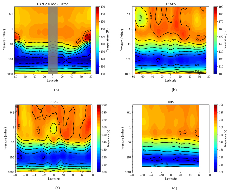
Figure 4. Zonally averaged temperature from observations and a dynamical model with a frictional drag force timescale τf of 200 days at the base linearly decreasing with altitude to 10 days at the top. The gray band represents the equatorial zone where our model lacks accuracy.
Download figure:
Standard image High-resolution imageFigure 5 shows the zonal, meridional, and vertical wind distributions, while Figure 6 shows the mass stream function. In the low to mid-latitudes, the zonal-mean zonal wind extends to the top of the stratosphere, decaying with height due to the frictional drag. Meridional motion is predominantly poleward above the tropopause, forming two equator-to-pole circulation cells. A smaller pole-to-mid-latitude cell appears in the northern hemisphere of the troposphere. Upwelling is maximal near zonal jets and reaches ∼0.05 mm s−1 at maximum, while downwelling is strongest near ± 65° at the top of the stratosphere. In general, the shape of our simulated mass stream function is qualitatively similar to what Conrath's dynamical model found for the stratosphere (see Figures 11 & 12 in Conrath et al. (1990)). Interestingly, the τf = 200 day case has multiple circulation cells in the northern middle and high latitudes above the 10 mbar level. A higher zonal wind velocity in the stratosphere for this case is a consequence of the comparatively lessened drag, which also allows local thermally-driven cells to develop in the polar region where the radiative influence of haze dominates.
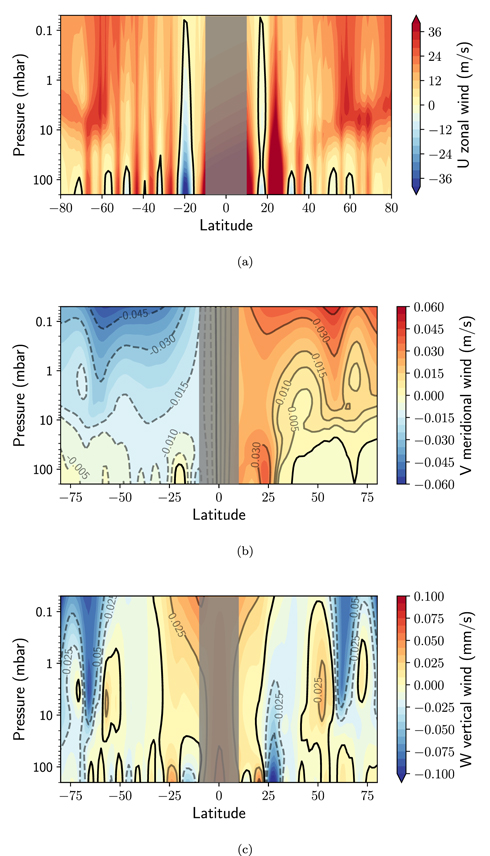
Figure 5. Contours of zonally averaged (a) zonal wind (m s−1), (b) meridional wind (m s−1), and (c) vertical wind (mm s−1), for the dynamical model (τf = 200 days at base, decreasing to 10 days at top). Solid lines mark transitions from positive to negative values, and dashed contours denote negative values. Zonal wind maxima are excluded to better show contrast in the mid-speed jets; the maxima occur at the base of the model at ± 11° and 25°N (130 m s−1), and the minimum at −20°S (−50 m s−1). The gray band represents the equatorial zone where our model lacks accuracy.
Download figure:
Standard image High-resolution image
Figure 6. Contours of the mass stream function for dynamical models; (a) τf = 200 days at base, decreasing to 10 days at top, and (b) τf = 200 days (uniform). Blue contours have negative values and generally represent anti-clockwise flow, while positive red contours represent clockwise flow. The gray band represents the equatorial zone where our model lacks accuracy.
Download figure:
Standard image High-resolution imageHowever, both simulated stream-function patterns look different from those produced by the post-analysis approach. Previous studies used the observed temperature, gas, and haze distributions to derive Jupiter's residual mean circulation (West et al. 1992; Moreno & Sedano 1997; Guerlet et al. 2020). Because these studies calculated different net radiative heating rates, they obtained various circulation patterns, except a special case with enhanced absorption and heating rates in polar haze (scenario #3 in Guerlet et al. 2020) that matched the stream function of West et al. (1992). This match probably occurs because West et al. (1992) ignored polar haze cooling.
Different circulation patterns also imply different Eliassen–Palm (E–P) flux divergence. The divergence of the E–P flux is approximated as  in a steady-state form of the momentum equation, where the eddy forcing on the zonal flow that accelerates and decelerates jets is proportional to the meridional velocity. E–P flux divergence derived from the post-analysis approach shows very complicated patterns, implying sophisticated wave-mean interactions. However, our assumed latitudinally uniform drag timescale could not capture the spatial variation of realistic wave forcing. The lack of realistic waves and uncertainty of the haze properties in our model limit our ability to accurately explain the exact pattern of latitudinal temperature distribution and the net heating rate, and thus the circulation, in the middle atmosphere of Jupiter. We leave a more detailed wave parameterization scheme on Jupiter for future work.
3.3. Effects of Polar Haze
Due to the large uncertainties in the haze radiative heating and cooling rates, here we examine the haze radiative effect on the temperature distribution and circulation patterns. We vary the haze IR opacity by a factor of two and also test a case with no haze cooling. For our nominal dynamical model (vertically increasing τf of 200 days at the base to 10 days at the top), the maximal influence of heating from the haze layer occurs near ± 80° and 3 mbar (Figure 4(a)). The dynamical model also results in more rapid drops of temperature poleward of ±60° between 10 and 50 mbar than observations. In Figure 7(a), we see that increasing haze IR opacity by 2× further decreases temperatures poleward of 60° above the 30 mbar level and reduces the magnitude and extent of the polar hotspots. The opposite extreme (Figure 7(d)), a case with no haze cooling, shows polar hotspots expanded in size and intensity, and generally warmer temperatures poleward of ± 60° above the 30 mbar level. In levels below, polar temperatures near the tropopause decrease with reduced haze IR opacity. This correlation between reduced haze IR opacity and (1) reduced cooling at the 15 mbar concentrated haze layer and (2) increased cooling at the tropopause (100 mbar) matches a similar conclusion in Zhang et al. (2015, Figure 6(b)). We also show that the change in cooling rate at the concentrated haze level affects the upper stratospheric temperature in polar regions due to the infrared radiative flux exchange. Equatorward of ± 50°, varying the haze IR opacity shows little effect on the temperature.

Figure 7. Contours of zonally averaged temperature for τf = 200 days at base, decreasing to 10 days at top, with (a) 2×, (b) 1×, (c) 0.5×, and (d) 0 haze IR opacity. The gray band represents the equatorial zone where our model lacks accuracy.
Download figure:
Standard image High-resolution imageThe case with increased 2× haze IR opacity, which resulted in cooler polar temperatures above 30 mbar, generates a circulation pattern with few differences from 1× opacity; the mass stream function is nearly identical (Figure 6(a) and Figure 8(a)). However, in the case with no haze cooling, two anti-circulation cells appear at 40–60°N (maximal in the troposphere) and 60°S (maximal at 5 mbar) (Figure 8(b)). Polar temperatures more than 20 K warmer than observations cause our simple frictional drag models to generate a more complex circulation pattern than a simple broad equator-to-pole pattern in the stratosphere. If multiple-cell circulation is truly present in Jupiter's middle atmosphere, as is suggested by the post-analysis studies (e.g., West et al. 1992; Guerlet et al. 2020), a better characterization of Jupiter's stratospheric and tropospheric hazes will be needed for a 2D dynamical model to produce accurate circulation.
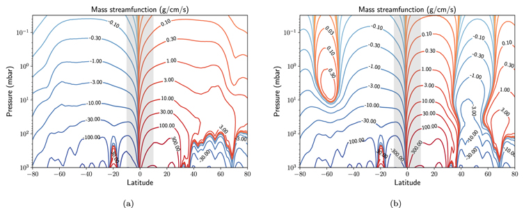
Figure 8. Contours of the mass stream function for τf = 200 days at base, decreasing to 10 days at top, with (a) 2×, and (b) zero haze IR opacity (i.e., no haze cooling). Blue contours represent negative values and generally represent anti-clockwise flow, while red contours represent clockwise flow. The gray band represents the equatorial zone where our model lacks accuracy.
Download figure:
Standard image High-resolution image
Figure A1. Key inputs in the model: (left) vertical profiles of C2H2 and C2H6, which are assumed uniform with latitude, (middle) contours of normalized zonal-mean stratospheric haze mixing ratio from Zhang et al. (2013b), and (right) the eddy diffusivity profile in the troposphere. The stratospheric haze heating and cooling rates are plotted in Figure 4 in Zhang et al. (2015) and the tropospheric counterpart is in Figure 6 in Guerlet et al. (2020).
Download figure:
Standard image High-resolution image
4. Conclusions and Discussion
By implementing a 2D dynamical model with accurate radiative transfer and most recent observations of temperature, global mean hydrocarbon abundances, and haze distribution, we perform a "first-principles" calculation of the circulation dynamics in Jupiter's middle atmosphere. We summarize the findings:
- 1.A radiative equilibrium with accurate radiative transfer can reproduce observed global mean temperature in the stratosphere. We find that in order to match the global mean temperature above 0.5 mbar, C2H2, and C2H6 abundances must be at the lower end of the uncertainty range.
- 2.Dynamics with a latitudinally uniform drag timescale τf = 2000 days similar to Conrath et al. (1990) introduces little latitudinal temperature variation. Forcing with 10× strength (τf = 200 days , decreasing to 10 days at the top of the atmosphere) increased latitudinal variability but still not as much as observations, suggesting realistic wave parameterization is needed to produce the observed 5–10 K variations.
- 3.Varying haze IR opacity has a noticeable effect on the haze cooling rates and polar temperatures throughout the middle atmosphere as well as the resulting meridional circulation in the high latitudes. Better constraints on observations of haze distribution and optical properties will be necessary for accurate characterization of diabatic forcing at high latitudes.
Although our radiative equilibrium model could reproduce observed globally averaged temperatures in the stratosphere with reduced abundances of C2H2 and C2H6 (Moses et al. 2004; Nixon et al. 2010; Zhang et al. 2013b), future studies should also search for other possible heat sources. It has been suggested that the upper stratosphere and thermosphere could be additionally heated (or cooled) by upwardly propagating gravity waves that dissipate between 10−4 and 10−7 mbar (Matcheva & Strobel 1999; Yelle & Miller 2004). High-energy charged particles have also been suggested to be responsible for heating at 1 mbar in the polar auroral region (Sinclair et al. 2017b). Also, the non-local thermodynamic equilibrium (non-LTE) effect might be important in the upper stratosphere and in the polar auroral region but was not considered in our current model (Zhang et al. 2013a).
Reproducing the observed latitudinal variations of temperature in Jupiter's middle atmosphere is the first step in understanding the radiative and mechanical forcing behind meridional circulation. Though the latitudinal variation of C2H2 and C2H6 in Jupiter's stratosphere causes localized net heating or cooling, we have shown that they cannot fully account for latitudinal temperature fluctuations in the mid-latitude region (Figure 2). Our dynamical model with a drag timescale τf = 200 days at the bottom decreasing toward 10 days at the top seems to be able to reproduce the ∼2 K variability seen in IRIS observations, but still underestimates the temperature variations in CIRS and TEXES data (∼5–10 K). This suggests that the appropriate characterization of eddy forcing is more complex than a simple linear drag parameterization. Specifically, convectively generated waves from the troposphere may be influencing the strongest variations in temperature in Jupiter's middle atmosphere.
The residual mean circulation pattern from the nominal "decreasing timescale with height" drag model shows broad, equator-to-pole transport above 100 mbar and a few circulation cells appearing closer to 1 bar (Figure 6(a)). We also show models with a larger drag timescale in the stratosphere develop alternating cells in the northern stratosphere (Figure 6(b)) due to a relatively large dominance of polar haze radiation. All of the frictional drag models produce different circulation patterns than the multi-cell, alternating poleward and equatorward meridional flow patterns generated using the post-analysis method (West et al. 1992; Guerlet et al. 2020), suggesting that realistic wave forcing parameterization is necessary to reproduce the circulation patterns in the middle atmosphere of Jupiter.
For the high-latitude region, characterization of Jupiter's polar haze appears to be essential for successfully modeling temperatures throughout the middle atmosphere. The haze distribution of Zhang et al. (2013b) and Guerlet et al. (2020) is necessary to produce sufficient warming at the poles in the 1–10 mbar region. The nominal (1×) haze IR opacity used in this model produces polar hotspots slightly higher in altitude and warmer in temperature than observations and overly cools the poles between 10 and 100 mbar. Reducing the IR opacity increases these maxima while increasing it lowers polar temperatures between 0.03 and 20 mbar. Matching observations exactly is unlikely, as the polar temperature distribution has changed significantly between the observations of CIRS (2000, early northern summer) and TEXES (2014, late northern summer). The true distribution of polar haze could also be different than our model assumes: Kedziora-Chudczer & Bailey (2011) found two polar haze populations above and below a depleted 10–20 mbar region. They also concluded that the extent and optical properties of haze layers are different at the north and south poles. Have polar haze conditions changed between 2000 and 2007? Further observations will be essential in constraining haze properties and other energetic processes such as high-energy particle heating in the polar region.
Lastly, the QQO in Jupiter's stratosphere undoubtedly affects the circulation. Like the QBO on Earth, QQO is thought to be a wave-driven phenomenon (Friedson 1999; Cosentino et al. 2017, 2020). The QQO could also have connections to temperature fluctuations in the mid-latitudes. The direct simulation of equatorial dynamics is not accurate using our quasi-geostrophic model but we can implement QQO forcing and test its effect on the meridional circulation in the mid-latitude and high latitudes. Future work will mainly focus on implementing parameterizations of Rossby waves and gravity waves (e.g., Friedson 1999; Cosentino et al. 2017) to study the influence of wave-mean flow interaction on zonal-mean temperature and meridional circulation. We will also include hydrocarbon chemistry and tracer transport in the model to understand the radiative feedback of meridionally transported species on the circulation. The SOCRATES model has included a chemical module in Earth studies (Brasseur et al. 1990), which can be adapted for use on Jupiter and other giant planets.
We dedicate this work to Dr. Adam P. Showman (1968–2020) in recognition of his fundamental contribution to the understanding of atmospheric dynamics on giant planets. N. G. Z. was supported by NASA Headquarters under the NASA Earth and Space Science Fellowship Program—Grant 80NSSC17K0479 and Grant NNX17AE27G. X. Z. was supported by NASA Solar System Workings grant NNX16AG08G. T. L. was supported by the Strategic Priority Research Program of the Chinese Academy of Sciences, Grant XDB 41000000, and the National Natural Science Foundation of China Grant 41974175.
Appendix A: Derivation of Residual Mean Stream-function Equation
We present the derivation of a stream-function equation from the zonally averaged, quasi-geostrophic equations of motion in Garcia & Solomon (1983):


 is the zonal-mean zonal velocity, and
  and
and  are the horizontal and vertical residual mean velocity components.
  is the local temperature deviation from the zonally averaged temperature. Q represents all radiative and diffusive heating components
  , and F represents all mechanical forcing components. N2 is the squared Brunt-Väisälä frequency from constant T, H is the constant scale height, a is planet radius, dy = ad
ϕ, with ϕ as latitude. Log-pressure altitude,
, and F represents all mechanical forcing components. N2 is the squared Brunt-Väisälä frequency from constant T, H is the constant scale height, a is planet radius, dy = ad
ϕ, with ϕ as latitude. Log-pressure altitude,  , and
, and  is the residual mean stream function. From here, we will drop ∗ notation.
Substitute (A7) and (A8) into the momentum Equation, (A1), and assume time derivatives  are 0 (steady state):
Multiply both sides by  , then take the partial derivative
  of all terms.
Multiply all terms by f:
Substitute (A7) and (A8) into the thermodynamic Equation, A3, again assuming time derivatives  are 0 (steady state):
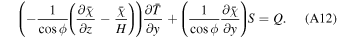
Take the partial derivative  of all terms, then multiply both sides by
  :
:
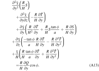
Substitute the thermal wind Equation, (A5), for  in (A13):
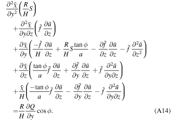
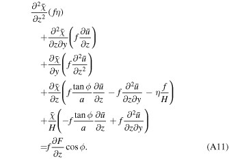
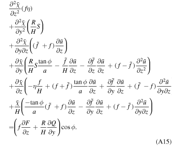
Sum (A14) with the momentum Equation, (A11), to form the stream-function equation:
We can compare parenthetical terms to C coefficients in Garcia & Solomon (1983, p. 14). To match, one must neglect the  term, assume
  , and assume that
  is needed in front of
  in the Garcia definition of CF
(the right-hand side of the stream-function equation). The
in the Garcia definition of CF
(the right-hand side of the stream-function equation). The  (Cχ
) term is consistent with Equation (12)f of a similar derivation in Choi et al. (1995) if the same assumptions about
(Cχ
) term is consistent with Equation (12)f of a similar derivation in Choi et al. (1995) if the same assumptions about  are made. The key inputs of our Jupiter model are plotted in Figure A1.