


Abstract
Models of solar-like oscillators yield acoustic modes at different frequencies than would be seen in actual stars possessing identical interior structure, due to modeling error near the surface. This asteroseismic "surface term" must be corrected when mode frequencies are used to infer stellar structure. Subgiants exhibit oscillations of mixed acoustic (p-mode) and gravity (g-mode) character, which defy description by the traditional p-mode asymptotic relation. Since nonparametric diagnostics of the surface term rely on this description, they cannot be applied to subgiants directly. In Paper I, we generalized such nonparametric methods to mixed modes, and showed that traditional surface-term corrections only account for mixed-mode coupling to, at best, first order in a perturbative expansion. Here, we apply those results, modeling subgiants using asteroseismic data. We demonstrate that, for grid-based inference of subgiant properties using individual mode frequencies, neglecting higher-order effects of mode coupling in the surface term results in significant systematic differences in the inferred stellar masses, and measurable systematics in other fundamental properties. While these systematics are smaller than those resulting from other choices of model construction, they persist for both parametric and nonparametric formulations of the surface term. This suggests that mode coupling should be fully accounted for when correcting for the surface term in seismic modeling with mixed modes, irrespective of the choice of correction used. The inferred properties of subgiants, in particular masses and ages, also depend on the choice of surface-term correction, in a different manner from those of both main-sequence and red giant stars.
Export citation and abstract BibTeX RIS
1. Introduction
Solar-like oscillators exhibit a characteristic comb-like pattern of peaks in the power spectra of their photometric or velocimetric time series, where each peak occurs at the natural frequency associated with a normal mode of oscillation. For pressure waves (p-modes) in Sun-like stars, the frequencies of these normal modes satisfy an approximate asymptotic relation (e.g., Tassoul 1994)

where n is the radial order of a mode, l is its angular degree,  l,n
is a phase offset, and Δν, the large frequency separation, is the characteristic frequency of the p-mode cavity. These frequencies depend on only the interior structure of these stars, and forward modeling is needed in order to constrain other stellar properties and physics, such as their ages and mixing parameters, which best reproduce this structure. On the other hand, detailed examination of the solar case reveals that the normal modes of standard solar models, with interior structures matching that of the Sun, have frequencies differing from the corresponding observed normal-mode oscillation frequencies. These frequency differences are thought to derive primarily from modeling errors localized to the solar surface (e.g., Christensen-Dalsgaard & Berthomieu 1991; Rosenthal et al. 1999), and therefore are collectively referred to as the solar "surface term." It is believed that such a surface term should also exist in seismically constrained models of other stars as well.
l,n
is a phase offset, and Δν, the large frequency separation, is the characteristic frequency of the p-mode cavity. These frequencies depend on only the interior structure of these stars, and forward modeling is needed in order to constrain other stellar properties and physics, such as their ages and mixing parameters, which best reproduce this structure. On the other hand, detailed examination of the solar case reveals that the normal modes of standard solar models, with interior structures matching that of the Sun, have frequencies differing from the corresponding observed normal-mode oscillation frequencies. These frequency differences are thought to derive primarily from modeling errors localized to the solar surface (e.g., Christensen-Dalsgaard & Berthomieu 1991; Rosenthal et al. 1999), and therefore are collectively referred to as the solar "surface term." It is believed that such a surface term should also exist in seismically constrained models of other stars as well.
These frequency differences must be accounted for when modeling stars to match observed mode frequencies, and many prescriptions exist to correct for or diagnose their effects. These include both parametric "surface term corrections," which describe the surface term as a slowly varying function of frequency (e.g., Kjeldsen et al. 2008; Ball & Gizon 2014; Sonoi et al. 2015), as well as nonparametric techniques, which exploit the structure of the asymptotic relation Equation (1) (Otí Floranes et al. 2005; Roxburgh 2005, 2016). Ong et al. (2021a) demonstrated that the inference of some stellar properties, such as stellar masses, radii, and ages, is robust to variations in choice of method on the main sequence, but exhibits nontrivial systematic dependence on surface-term methodology for a sample of red giants. They suggested that the difference between the two regimes might be illuminated by examining stars in an intermediate stage of evolution—subgiants.
Subgiants are of particular interest in the asteroseismic context. Generally speaking, nonradial modes can be classified into p-modes propagating in the exterior of a star, and internal gravity waves (g-modes) propagating in its radiative interior (Unno et al. 1989). The evolution of stars off the main sequence causes the maximum Brunt–Väisälä frequency of the interior g-mode cavity to increase rapidly as the star expands, and its radiative core contracts, in the process of crossing the Hertzsprung gap. As these g-modes approach the frequencies of the p-modes, they couple to produce modes of mixed character, resulting in a forest of avoided crossings (Aizenman et al. 1977). The specific configurations of these "mixed modes" strongly constrain the interior structure of the star, especially near the evanescent region between the two mode cavities (e.g., Deheuvels & Michel 2011; Noll et al. 2021).
Subgiants are also astrophysically interesting in a broader sense, insofar as they may shed light on the physics underlying post-main-sequence evolution (see Godoy-Rivera et al. 2021, and references therein), the evolution of planetary systems that they may host (e.g., Huber et al. 2019), or the histories of the stellar populations of which they are members (e.g., Chaplin et al. 2020). Historically, they have been less well studied than both main-sequence stars and red giants as a result of unfavourable observational selection functions: they are both much less common than main-sequence stars and much fainter than red giants. However, for detailed asteroseismic characterization, these considerations are in some ways reversed: they are at once more observationally accessible than main-sequence stars (in consequence of larger photometric amplitudes and longer dynamical timescales) and more computationally tractable than red giants (see Silva Aguirre et al. 2020, Christensen-Dalsgaard et al. 2020). For this reason, subgiants constitute a nontrivial portion of the asteroseismic targets for the Transiting Exoplanet Survey Satellite (TESS, Schofield et al. 2019) mission. The upcoming PLATO mission (Rauer et al. 2014) is expected to yield even more subgiant targets amenable to seismic analysis.
However, mixed modes in subgiants raise methodological issues, in that they cease to satisfy Equation (1). Since the theoretical constructions underlying nonparametric characterizations of the surface term rely on Equation (1), which strictly applies only to p-modes, these techniques are applicable only to the extent that Equation (1) is valid; in their unmodified form they are therefore inapplicable to mixed modes. Additionally, existing parametric surface-term corrections have all been developed for p-modes, and the theoretical basis for applying them to mixed modes has hitherto been less certain. These methodological concerns must be addressed if detailed seismic characterization of subgiants, in spite of the surface term, is to be credible.
While mixed modes have been observed in both subgiants and red giants, such mode mixing has so far been much less of an issue in red giants. Traditionally, descriptions of the coupling between the two mode cavities have relied on the Jeffreys–Wentzel–Kramers–Brillouin (JWKB) approximation (Takata 2016; Pinćon et al. 2020), which describes the interior g-mode cavities in evolved red giants extremely well. In this regime, the density of mixed modes is sufficiently high, and the coupling between the two mode cavities is also sufficiently weak, that the modes with the highest local amplitudes behave essentially like p-modes (e.g., Aerts et al. 2010). For quadrupole and higher-degree modes, this permits mode mixing to be essentially ignored, and nonparametric methods to be applied to the most p-dominated mixed modes as if they were pure p-modes, with little loss of accuracy (Ball et al. 2018; Jørgensen et al. 2020; Ong et al. 2021a). Unfortunately, none of these conditions hold in subgiants. Consequently, the generalization of nonparametric treatments of the surface term to mixed modes in the strongly nonasymptotic regime, which is necessary for analysis of subgiants and for dipole mixed modes in red giants, has been a longstanding open theoretical and methodological problem.
In the companion paper to this work (Ong et al. 2021b, hereafter Paper I), we derived a generalization for one class of nonparametric treatments of the surface term—that of l
-matching, in the sense of Roxburgh (2016). Assuming that a nonparametric diagnostic for the surface term of this kind can be determined for the pure p-modes, we prescribed an analogous likelihood function for mixed modes, which quantifies whether a set of differences between observed and model mixed modes is consistent both with a surface-localized structural perturbation and with the eigenvalue equation of the internal coupling matrices associated with the stellar model (Ong & Basu 2020, hereafter OB20). In the process of doing so, we also derived generalizations of some existing parametric descriptions—in particular that of Ball & Gizon (2014, hereafter BG14)—to fully account for mixed-mode coupling, within the coupling-matrix construction. This algebraic approach does not rely on the JWKB approximation, and therefore is suitable for application to subgiants, unlike existing techniques.
In this work, we investigate the viability of these generalized prescriptions in the inverse direction—applying them in inferring the global and structural properties of subgiants. We will examine systematic differences in the inferred values of global parameters—masses, radii, ages, and initial helium abundances—as returned from different treatments of the surface term, all else being equal. In this manner, we fill in the existing gap between previous characterizations of surface-related modeling systematics on the main sequence (Basu & Kinnane 2018; Compton et al. 2018; Nsamba et al. 2018) and in red giants (Jørgensen et al. 2020; Ong et al. 2021a). We describe our modeling procedure in Section 2 and our subgiant sample in Section 3. In Section 4, we perform statistical tests to ascertain the relative sizes of various systematic effects; in Section 5 we discuss the implications that these results may have for the use of individual mode frequencies in stellar modeling, and make recommendations for best practices going forward.
2. Modelling Procedure
While there exists significant methodological variability in how such seismic modeling is to be done, we can, broadly speaking, make a distinction between large-scale multi-target grid searches (as in, e.g., McKeever et al. 2019; Jørgensen et al.2020; Li et al. 2020a; Nsamba et al. 2021; Ong et al. 2021a) and more "boutique" target-by-target modeling (as in, e.g., Ball et al. 2018, 2020; Huber et al. 2019; Chaplin et al. 2020; Noll et al. 2021). In the former case, a precomputed grid of stellar models spanning a reasonably large parameter space is used, and the goal of the modeling exercise is to search for the model within the grid that best matches a set of observational constraints, for each target in the sample. Conversely, in the latter case, the region of parameter space being searched is adapted to each target, and hence is much smaller; the stellar models used in the procedure are also typically constructed ad hoc for each target. These two approaches are not necessarily mutually exclusive. The results of grid searches may be used to restrict the region of parameter space being considered for more refined analysis. While boutique modeling often involves an optimization-based parameter search, it is also not uncommon to construct more finely-sampled "detailed" grids adapted to individual targets. For this study, however, we restrict our attention to the former case, using a single precomputed model grid for all stars.
2.1. Model Grids
We construct a grid of subgiant models with mesa (Paxton et al. 2011, 2013, 2018) version 12778, using Eddington-gray atmospheres and the solar elemental mixture of Grevesse & Sauval (1998). The parameters of the grid were the stellar mass (in the range M ∈ [0.8 M⊙, 2.0 M⊙]), initial helium abundance (Y0 ∈ [0.248, 0.32]), initial metallicity ([Fe/H]0 ∈ [–1, 0.5]), the mixing length parameter (αMLT ∈ [1.3, 2.2]), and the core step overshoot parameter fov, whose distribution we describe in more detail below. Diffusion and settling of helium and heavy elements were handled using the formulation of Thoul et al. (1994), with an additional mass-dependent prefactor to the diffusion coefficient (as prescribed in Viani et al. 2018) to smoothly disable diffusion at higher masses. For each evolutionary track, we retained stellar models starting when  (i.e., where the local spacing of dipole g-modes is comparable to
  ) and ending when Δν = 9 μHz.
The first four of these grid parameters were distributed uniformly using joint Sobol sequences of length 213 − 1 =8191 over the parameter space described above. For the overshoot parameters, we opted to use the mass-overshoot relation of Viani & Basu (2020), rather than specifying values of fov uniformly using Sobol sequences. In order to do so, we needed to translate between the different implementations of step overshooting in YREC (Demarque et al. 2008)—the stellar evolution code used in Viani & Basu (2020)—and mesa, as well as between different definitions of how the input values of the overshoot parameter are related to the final, effective overshooting distance. In particular, the main results of Viani & Basu (2020) concern YREC's implementation of instantaneous overshoot mixing, in which the convective boundary for a convective core of size Rcz is extended outward by a distance

by directly modifying the superadiabatic gradient ∇ – ∇ad before solving the structure equations; here Hp is the pressure scale height at the convective boundary. Note that this "effective" overshooting distance is different from the nominal "input" overshooting length fov Hp ; the mass-overshoot relation of Viani & Basu (2020) yields values of feff = Lov/Hp as a function of stellar mass, rather than fov per se. In contrast, mesa implements diffusive overshoot mixing (or "overmixing") following the prescription of Herwig (2000), where the effective diffusion coefficient D for the mixing-length-theory treatment of convection, which would otherwise vanish outside the convective core, is artificially increased. In mesa's "step overshoot" mode, this is set to a uniform value D0 = D(Rcz −f0 Hp ) for a region extending

outward from the convective core boundary, where αov is a free parameter, which we set to 1 for our computations.
To reconcile these differences, for each star in the sample of Viani & Basu (2020), we constructed mesa models with identical global properties and input physics to their corresponding YREC models, for a range of input values of fov. For each of these models we found Lov, and therefore feff, directly by comparison with a fiducial model that was constructed with fov = 0. We then solved for the values of fov that yielded the same values of feff as the YREC models used in Viani & Basu (2020). We show the results of doing this in Figure 1. From this, we fitted a mass-overshoot relation with respect to the input values of fov (black line). For each point in this grid, we then sampled fov randomly from the ±2σ region around this fitted mass-overshoot relation (shown with orange points in Figure 1), treating negative values as 0.
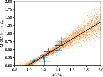
Figure 1. Input core overshoot values used in the model grid. The sample of Viani & Basu (2020) is shown with the blue points, with a fitted line shown in black. We distribute values of fov within the 2σ region around the fitted curve (orange points).
Download figure:
Standard image High-resolution imageFor each model in the grid i and star j, we construct a cost function
where the final term is a seismic cost function determined by the choice of surface term correction under consideration. Note that while Δν is not directly used as a constraint on the stellar models, it nonetheless enters into the seismic constraint indirectly. Following Viani et al. (2019), for this purpose we used the value of Δν obtained by fitting a linear relation of the form of Equation (1) to the radial p-modes, rather than using values determined by analysis of the raw power spectrum. For each star we then derived posterior distributions from these cost functions using the same Bayesian Monte Carlo grid-search procedure as in Ong et al. (2021a), except for the following specific modifications required to accommodate subgiants in particular.
2.2. Frequencies, Coupling Matrices, and Surface Corrections
As in Ong et al. (2021a), we compare the BG14 parameterization of the surface term, as our fiducial parameterization, with the -matching algorithm of Roxburgh (2016), which is nonparametric. In addition to directly comparing the two methods per se, we also compare two different approaches to mode coupling. As described in Paper I, all extant parameterizations of the surface term (including that of BG14) account for mode coupling indirectly, if they do at all, via weighting the surface-induced frequency perturbation by the mode inertia:

In Paper I, we showed that expressions of this form correspond to truncating a perturbative series describing the coupling between the p- and g-mode cavities, with respect to the natural basis of π- and γ-modes (in the sense of Aizenman et al. 1977; Ong & Basu 2020), to first order in the coupling strengths. In this construction the surface term is understood to result from the action of some undetermined structural perturbation operator, which is annihilated on the γ-mode subspace. The approximations that are implicit in this sort of truncation are not always valid; Paper I demonstrates that they hold good for young subgiants with strong coupling, and fail for very evolved red giant stars. Without any a priori constraints on the nature of the surface modeling error, however, it is difficult to say for sure whether or not these approximations hold good on the sample of subgiants under consideration here.
We thus compare the first-order approach to mode coupling, Equation (5), with the use of the full matrix construction presented in Ong & Basu (2020). Paper I provided the full details of the numerical framework required to perform this computation, and derived generalizations of both the BG14 parameterization and the -matching technique that account fully for mode coupling. For this work, we will compare the following surface corrections:
- 1.
- 2.Using the same parameters, we also evaluate a cost function applying a matrix-based generalization of the BG14 correction. We compute a χ2 statistic with contributions from the corrected radial and quadrupole p-modes using Equation (6), but for the dipole modes we compute corrected frequencies fully accounting for mixed-mode coupling (via Equations (8) and (18) of Paper I).
- 3.We also compute a nonparametric cost function by-matching, accounting for mode mixing to first order as described in Section 3.1 of Paper I.
- 4.Finally, we perform-matching while fully accounting for mode coupling, as described in Section 3.3 of Paper I.

For this purpose, we computed both the π- and γ-mode frequencies and mixed-mode coupling matrices via the mode isolation construction of OB20, as well as the mixed-mode frequencies themselves, for p-modes within ±6Δν of  . These computations were done using the stellar pulsation code gyre (Townsend & Teitler 2013). We used only the mixed-mode and π-mode frequencies for surface corrections, which account for mode coupling to first order (1 and 3). In order to address issues of matrix completeness where the matrix construction was required (2 and 4), we compute γ-mode frequencies and matrix elements for γ-modes from a frequency of
  all the way up to the ng
= 1 γ-mode, whose frequency is bounded from above by the maximum value of the Brunt–Väisälä frequency N as
all the way up to the ng
= 1 γ-mode, whose frequency is bounded from above by the maximum value of the Brunt–Väisälä frequency N as  . Since this is potentially much higher than the highest-frequency p-mode in the observational range, we restricted the effective matrix to omit the highest-frequency n0
γ-modes, where n0 was chosen to minimize the sum of squared differences between the mixed modes returned from the coupling eigenvalue equation and those returned directly from gyre. This was only done when the ng
= 1 γ-mode was higher in frequency than the highest π-mode frequency in the incomplete coupling matrix.
. Since this is potentially much higher than the highest-frequency p-mode in the observational range, we restricted the effective matrix to omit the highest-frequency n0
γ-modes, where n0 was chosen to minimize the sum of squared differences between the mixed modes returned from the coupling eigenvalue equation and those returned directly from gyre. This was only done when the ng
= 1 γ-mode was higher in frequency than the highest π-mode frequency in the incomplete coupling matrix.
The surface-corrected frequencies were then used to compute a cost function of the form

where σν,eff quantifies the systematic error in the modeling procedure owing to grid undersampling (see the next section).
As the computation of the corrected mode frequencies using the coupling-matrix eigenvalues is considerably more expensive than the first-order computation, we restricted this computation to only models that were both within a spectroscopic Mahalanobis distance of 25 (i.e., within 5σ) from the nominal spectroscopic constraints, and with Δν and  within 25% of the observational values. For each star, we assigned models outside this region a likelihood of 0.
2.3. Undersampling of Parameter Space
Subgiants pose a significant challenge for grid-based modeling because the evolution of their mode frequencies through avoided crossings is very rapid compared to the changes undergone by their pure p- and g-mode frequencies, considered separately (Deheuvels & Michel 2011). These avoided crossings also amplify systematic dependences of the inferred stellar properties on model parameters such as the convective mixing length. At this time, explicitly increasing the sampling density of model grids to match the typical frequency measurement errors remains prohibitively expensive to perform on a large scale.
For p-modes, such as the pure p-modes seen in main-sequence stars or p-dominated mixed modes in red giants, the effective parameter sampling density of model grids can be significantly improved by multivariate interpolation (e.g., Rendle et al. 2019). Numerical stability in this interpolation problem is achieved by constructing interpolants for the dimensionless phase quantities l,n
of Equation (1), rather than the mode frequencies themselves. By doing so, the interpolants better describe subtle changes in internal structure reflected in individual modes. This is as opposed to changes in mode frequencies that result from homology transformations, which instead affect all modes by rescaling the overall characteristic frequency Δν, which in turn may be interpolated separately.
Since avoided crossings in subgiants are not well described by a single characteristic frequency scale, their frequencies cannot be preconditioned for interpolation in this manner. Interpolation of subgiant models therefore requires model grids of already high sampling density, as shown in Li et al. (2020a). Moreover, the characteristic frequencies of both the p- and g-mode cavities each evolve rapidly as the subgiants cross the Hertzsprung gap. Consequently, while very high temporal and parameter sampling is required to match the strong structural constraints imposed by typical observational precision on the mode frequencies, conventional methods of increasing the effective grid sampling density fail in this regime of rapid evolution.
Li et al. (2020a) treat this by systematically inflating the effective measurement errors associated with the mode frequency measurements to match the parameter sampling of the grid. This effectively downweights the seismic cost term in Equation (4) relative to the classical spectroscopic constraints. We adopt a similar measure in our procedure. For each star, we first identify the best-fitting model in the grid, using Equation (7) with σν,eff set to zero. We then estimate the effective systematic frequency error σν,eff as the rms difference between the surface-corrected and observed mode frequencies for this best-fitting model in the grid, and add this in quadrature to the nominal frequency measurement errors when evaluating the posterior distribution functions in all subsequent calculations. Unlike Li et al. (2020a), we use a single value of this undersampling error for modes of all degrees l.
2.4. Regularization
Finally, it is a known property of the surface term that the differences between observed and model p-mode frequencies should decrease in magnitude at low frequencies for models with matching interior structures to the corresponding stars. Basu & Kinnane (2018) note that the seismic likelihood functions from different surface-term treatments may not adequately penalise stellar models in the grid that do not satisfy this property, necessitating further regularization. As in Basu & Kinnane (2018) and Ong et al. (2021a), we introduce an additional penalty function

over the lowest N uncorrected model frequencies. For this work we choose N = 4. Since this contribution to the cost function only serves the purpose of regularization, and is not meant to significantly influence the overall posterior distribution, we downweight it by a factor of 100.
3. Subgiant Sample
Mode frequencies of subgiants exhibit a broad range of observational characteristics, as their mixed modes span the transition from being largely p-dominated and interrupted by a sparse set of g-modes to being largely g-dominated and interrupted by a sparse set of p-modes. The transition between these two regimes is described by the ratio between the characteristic frequency spacings of the p-mode and g-mode cavities,  . This quantity exhibits a strong dependence on Δν. As such, for this study we model subgiants across a large range of Δν. At high Δν we have stars barely off the main sequence, whose subgiant status we diagnose with the presence of individually identifiable avoided crossings. At lower frequencies, we have stars partway up the red giant branch, where we adopt a minimum Δν of 15 μHz for inclusion in our sample. Additionally, we include in our sample stars that were observed by different space missions. In total, our subgiant sample consists of 36 stars observed with Kepler, six stars observed with TESS, and five subgiants observed with K2. We describe each of these subsamples in more detail below.
3.1. Kepler Subgiants
Photometry from the nominal Kepler mission, spanning its full duration of just over 4 yr, represents the best possible scenario for photometric measurements of oscillatory variability in solar-like pulsators. The long duration and high completeness of these time series ensure high resolution in their power spectra with relatively clean spectral line-spread functions, while the comparatively high sampling frequency of short-cadence observations (which is much higher than  ) reduces signal apodisation when measuring the oscillations of subgiants and main-sequence stars.
For this work, we consider a sample of subgiants observed at short cadence that has previously been subject to grid-based modeling with detailed seismic constraints (Li et al. 2020a, 2020b). For these targets, we use the global seismic properties Δν and  as derived by Serenelli et al. (2017), and the consolidated spectroscopic observables (Teff and [Fe/H]) from Table 1 of Li et al. (2020a). For detailed modeling, we also use the mode frequencies measured in Li et al. (2020b).
Table 1. Consolidated Spectroscopic and Seismic Constraints for TESS Subgiants
| Object | Teff/K |

| [Fe/H] (dex) | σ[Fe/H] (dex) | L/L⊙ | σL /L⊙ | Δν/μHz | σΔν /μHz |

|

| Reference |
|---|---|---|---|---|---|---|---|---|---|---|---|
| HD 38529 | 5578 | 52 | +0.34 | 0.06 | 6.233 | 0.149 | 36.68 | 0.82 | 624 | 20 | 1 |
| β Hyi | 5874 | 74 | −0.10 | 0.09 | 3.494 | 0.087 | 57.85 | 0.15 | ⋯ | ⋯ | 2 |
| ν Ind | 5320 | 64 | −1.18 a | 0.11 | 6.000 | 0.350 | 25.10 | 0.10 | ⋯ | ⋯ | 3 |
| δ Eri | 4954 | 30 | +0.06 | 0.05 | ⋯ | ⋯ | 40.58 | 0.14 | 669 | 7 | 4 |
| TOI-197 | 5080 | 90 | −0.08 | 0.08 | 5.150 | 0.170 | 28.94 | 0.15 | 430 | 18 | 5 |
| η Cep | 4970 | 100 | −0.09 a | 0.11 | 8.130 | 0.290 | 17.23 | 0.05 | 228 | 2 | 6 |
Note.
a Corrected for α-enrichment by prescription of Salaris et al. (1993).References. 1. Ball et al. (2020); 2. T. R. White et al. (2021, in preparation); 3. Chaplin et al. (2020); 4. E. P. Bellinger et al. (2021, in preparation); 5. Huber et al. (2019); 6. M. P. Joyce et al. (2021, in preparation).
Download table as: ASCIITypeset image
3.2. TESS Subgiants
We also consider a sample of subgiants observed with TESS during its nominal mission. This represents the opposite extreme of very short time series, where typically only a handful of modes can be detected (if at all). In the worst case, some of these subgiants have continuous photometry spanning only a single sector (27 days), which is not appreciably longer than the average mode lifetimes. Equivalently, in the frequency domain, the spectral resolution of the power spectrum—and thus the correlation frequency scale of the underlying correlated realisation noise—is comparable to the excited mode line widths. Consequently, the power spectra and fitted frequencies of these targets are far more sensitive to realisation noise than the Kepler sample. To make matters worse, TESS pixels are significantly larger than Kepler ones, and therefore potentially suffer more contamination from nearby objects. Generically speaking, the detection and extraction of seismic characteristics from these short and relatively contaminated power spectra—let alone individual mode frequencies—is a challenging task.
Since photometric and time-series data analysis in this very difficult regime is not the focus of this work, we restrict our attention to only a relatively small sample of TESS subgiant oscillators for which mode frequencies have previously been identified by and circulated within the asteroseismology community. These are TOI-197 (Huber et al. 2019), ν Ind (Chaplin et al. 2020), β Hyi (T. R. White et al. 2021, in preparation), δ Eri (E. P. Bellinger et al. 2021, in preparation), HD 38529 (Ball et al. 2020), and η Cep (M. P. Joyce et al. 2021, in preparation). We show their consolidated spectroscopic and global seismic properties in Table 1.
3.3. K2 Subgiants
Data from the K2 mission lie in between these two extremes. On one hand, the time series available from K2 span 80 days in each campaign (as opposed to 27 days in a TESS sector), with 60 s sampling at short cadence (as opposed to TESS's 2 minutes). On the other hand, the pointing stability (and thus photometric noise) of these time series is much degraded compared to the nominal Kepler mission, owing to the drift-scanning strategy across the ecliptic plane adopted by K2, necessitated by loss of attitude control. For our sample, we use a set of K2 short-cadence stars observed across multiple campaigns for which a significant oscillation power excess could be identified by visual inspection of their photometric power spectra. The oscillation frequencies and spectroscopic properties of these stars have not been previously published; we describe them in detail below.
3.3.1. Spectroscopic Constraints
Single spectra for each of these targets were obtained between UT 2017 June 9 and June 12, using the Tillinghast Reflector Echelle Spectrograph (TRES, see Fűrész 2008; Mink 2011) on the 1.5 m telescope at the Fred L. Whipple Observatory (FLWO) on Mt. Hopkins in Arizona. TRES is an optical echelle spectrograph with a wavelength range 385–910 nm and a resolving power of R ∼ 44,000. The TRES spectra were extracted using procedures described in Buchhave et al. (2010), and then used to derive stellar effective temperatures (Teff), metallicities ([M/H]), and surface gravities ( ) using the Stellar Parameter Classification tool (SPC, see Buchhave et al. 2012) without any stellar isochrone models as a prior. SPC cross-correlates an observed spectrum against a grid of synthetic spectra based on Kurucz atmospheric models (Kurucz 1992).
For each star, an initial set of spectroscopic parameters was derived by permitting each parameter to vary freely in the fit. As done in Lund et al. (2016), the resulting value of Teff was then used to calculate a new value of the surface gravity consistent with  obtained from their photometric power spectra (described in the following section), via the solar-calibrated
  scaling relation (Kjeldsen & Bedding 1995)
This seismic value of  (calibrated against the solar value of g = 27,402 cm s−1, from Campante et al. 2014) was then used to perform another SPC analysis, run with
  as a fixed parameter, yielding a final set of spectroscopic values.
3.3.2. Power Spectra and Seismic Constraints
We use power spectra derived from photometric time series, which were in turn processed using the K2P2 pipeline (Lund et al. 2015) with custom apertures in order to ameliorate CCD bleeding, and corrected using the KASOC filter (Handberg & Lund 2014). Weighted Lomb–Scargle power spectra were computed for each campaign separately out of the K2P2 time series, with each point in the time series weighted by the rms photometric variability within a symmetric 2 day running filter. A final power spectrum was then made from a weighted average of the power spectra from individual campaigns. For a more detailed description, see M. N. Lund et al. (2021, in preparation).
From these combined power spectra, the global seismic parameters Δν and  were found using the 'coefficient of variation' method of Bell et al. (2019). The value of Δν found here was only used as an initial estimate to seed the mode identification for peak-bagging; for modeling purposes we refit Δν as described above. Mode frequencies were then fitted against these power spectra using a combination of techniques. Radial and quadrupole modes were identified and fitted using PBJam (Nielsen et al. 2021); dipole modes were identified by hand by visual inspection of the replicated echelle diagrams (Bedding 2012) and fitted using diamonds (Corsaro & De Ridder 2014). For modeling we retained only modes with a peak signal-to-noise ratio larger than 25.
We show the consolidated spectroscopic and seismic properties of these K2 stars in Table 2, and their mode frequencies in Table 4 in the Appendix. Of the 11 stars in the original sample, four were main-sequence stars (with Δν between 65 μHz and 133 μHz and no discernible mode mixing), and two were red giants (Δν < 15 μHz). We excluded these from consideration for our grid-based modeling.
Table 2. Consolidated Spectroscopic and Seismic Constraints for our K2 Sample
| EPIC | Teff/K | [M/H] (dex) | Δν/μHz | σΔν /μHz |
 /μHz /μHz |
 /μHz /μHz | L/L⊙ | σL /L⊙ |
|---|---|---|---|---|---|---|---|---|
| 212478598 | 5058 | −0.356 | 35.09 | 0.05 | 536.7 | 4.8 | ⋯ | ⋯ |
| 212485100 | 6169 | −0.041 | 87.34 | 0.12 | 1834.3 | 21.4 | ⋯ | ⋯ |
| 212487676 | 6036 | −0.314 | 75.89 | 0.21 | 1448.2 | 14.5 | 2.651 | 0.023 |
| 212516207 | 6253 | +0.130 | 68.02 | 0.26 | 1373.6 | 20.0 | 4.031 | 0.042 |
| 212586030 | 4895 | +0.230 | 21.70 | 0.03 | 311.5 | 10.0 | 6.079 | 0.273 |
| 212683142 | 5898 | −0.052 | 45.76 | 0.05 | 806.1 | 8.3 | 5.670 | 0.052 |
| 212708252 | 5616 | −0.095 | 132.95 | 0.26 | 2896.7 | 21.7 | 0.887 | 0.003 |
| 246154489 | 5018 | −0.355 | 14.28 | 0.03 | 187.5 | 4.4 | 12.38 | 0.12 |
| 246184564 | 4932 | −0.131 | 11.82 | 0.02 | 155.4 | 5.4 | 16.94 | 0.25 |
| 246305274 | 6178 | −0.431 | 46.60 | 0.24 | 795.2 | 12.3 | ⋯ | ⋯ |
| 246305350 | 5991 | +0.011 | 48.00 | 0.18 | 831.7 | 13.6 | 5.767 | 0.051 |
Note. We adopted a uniform value of  and σ[M/H] = 0.08 dex. Luminosities are from Gaia Collaboration et al. (2018).
Download table as: ASCIITypeset image
4. Results
For stellar models that provide good matches to the internal structure of the observed stars, we find that the differences between the corrected frequencies implied by each of the surface-term treatments we have considered here can be quite subtle. We show a representative example in Figure 2, which is the best-fitting model for EPIC 212478598 with respect to the first-order BG14 correction. In the neighborhood of  , the different corrections yield (at least visually) very similar results on the dipole mixed modes. Variations in the posterior distributions do not originate from how they respond to surface-localized structural differences, because by construction such frequency errors should lie mainly in the nullspace of all of these cost functions if the surface term is small. Instead, they result from "false positives": differences in how these prescriptions might fail to penalise interior structural differences between the star and the model. It is difficult to say a priori, from strictly theoretical considerations, how the inferred stellar properties might respond to these differences, all else being equal. This is why explicit comparisons of the inferred properties are required.
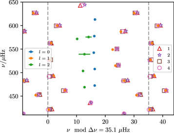
Figure 2. Replicated echelle diagram of EPIC 212478598, showing observed modes as points colored by angular degree, and model l = 1 frequencies corrected with various prescriptions for the surface term with the open symbols. With respect to the descriptions in Section 2.2: we show correction 1 with the upright triangles, 2 with the stars, 3 with the squares, and 4 with the open circles.
Download figure:
Standard image High-resolution imageFollowing Ong et al. (2021a), we compare the different modeling methods by way of the normalized differences between them. For a given property (e.g., the stellar mass M), we define a normalized score, e.g. zM
, as the differences between the posterior mean values μM
as reported by two different estimation methods A and B, normalized by the combination in quadrature of their reported uncertainties, for which we use their posterior variances  :
:
Under the null hypothesis that estimation methods A and B are consistent with each other, these z-scores should be distributed with a population mean of 0. Our alternative hypothesis, that A and B are not consistent with each other, does not constrain the sign of the population mean of z. Consequently, we perform one-sample two-tailed t-tests of this null hypothesis, following Silva Aguirre et al. (2017) and Ong et al. (2021a). As in Ong et al. (2021a) we adopt a 3σ level of significance (i.e., we reject the null hypothesis for p ≲ 0.0025). We perform comparisons of this kind on some fundamental stellar properties that are of astrophysical interest: the stellar masses, radii, ages, and initial helium abundances. We show the p-values associated with various comparisons that we performed in Table 3. In the next few sections, we explain each set of comparisons in detail.
Table 3. t-test p-values
| Quantity | First-order versus Full | BG14 versus -matching | L versus No L | This Work versus Li et al. (2020a) | ||||
|---|---|---|---|---|---|---|---|---|
| BG14 (1 versus 2) |
-match (3 versus 4) | 1st order (1 versus 3) | Full (2 versus 4) | Full with L | BG14 (2) |
-match (4) | BG14 (1), without L | |
| Mass | 7.588 × 10⁻⁵ | 0.0009 | 0.3473 | 0.0009 | 0.4787 | 0.9921 | 0.0851 | 0.0016 |
| Radius | 0.0139 | 0.0267 | 0.0150 | 0.0220 | 0.3061 | 0.6420 | 0.0044 | 0.0445 |
| Age | 0.8918 | 0.7374 | 0.0003 | 0.0037 | 0.9041 | 0.9008 | 0.0371 | 0.0094 |
| Y0 | 0.0024 | 0.0258 | 0.1117 | 0.3904 | 0.0754 | 0.1526 | 0.9241 | ⋯ |
Note. p-values are for differences between modelling methodologies, under the null hypothesis that the normalized differences z, Equation (10), are distributed with a population mean of 0. If p < α = 0.0025, then estimates of a given property returned by two different methods are on average not consistent with each other at the 3σ level; these are indicated with bold face
.
Download table as: ASCIITypeset image
4.1. Full versus First-order Mode Coupling
The second and third columns of Table 3 describe comparisons between theoretical constructions of the surface term that are identical save for how mode coupling is handled. In the second column, we compare the first-order and full matrix generalization of the BG14 surface term (corrections 1 and 2 of Section 2.2), and in the third we compare the first-order and full matrix generalization of the -matching algorithm (corrections 3 and 4). These correspond to the pairwise comparisons and cumulative distribution functions (CDFs) of z-scores shown in Figure 3.
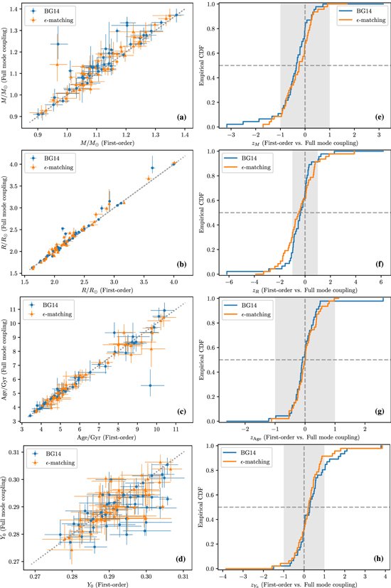
Figure 3. Comparisons between properties estimated using first-order and full treatments of mode coupling for two different surface-term corrections. In parts (a)–(d) (left column) we show a direct comparison between first-order (horizontal axis) and full (vertical) mode coupling calculations, with points showing the median of the posterior distribution, colored by theoretical prescription. The line of equality is shown with the gray dotted line in the background. In parts (e)–(h) (right column) we show the empirical cumulative distributions of the normalized differences, per Equation (10). We show the ±1σ interval with the shaded region. Dashed lines indicate z = 0 and the theoretical median (p = 0.5) of the CDF.
Download figure:
Standard image High-resolution imageIn each of these cases we find that the reported values of the stellar mass differ significantly within each pair. We also see a similar (albeit somewhat marginally significant) difference in the inferred initial helium abundances for the BG14 correction, but not for -matching. We attribute this discrepancy to -matching returning somewhat larger posterior uncertainties in general, since it places considerably weaker constraints on the functional form of the surface term in consequence of its nonparametric nature. These differences indicate that explicitly accounting for mode coupling to beyond first order when computing corrections for the surface term may be necessary for estimating masses and helium abundances of evolved stars with mixed modes, even given the present limitations of grid-based modeling.
We do not obtain any other statistically significant differences of this kind. This does not necessarily imply that first-order and full treatments of mode coupling return equivalent results; the only conclusion we may draw is that even if any such differences exist, the limitations of both the observational precision and intrinsic systematic errors in our grid-based modeling are more severe than would permit them to be demonstrated at the 3σ level by the techniques we have used.
4.2. Parametric versus Nonparametric Treatment
In the fourth and fifth columns of Table 3 we show the results of comparing different formulations of the surface term, keeping the treatment of mode coupling the same. In the fourth column we compare the surface correction of BG14 against the -matching algorithm, in both cases only accounting for mode mixing to first order; in the fifth we compare these methods as computed with respect to the coupling-matrix eigenvalue equation.
We see significant systematic effects in the inferred masses and ages, which we show in panels (a), (b), (e), and (f) of Figure 4. These results are slightly harder to interpret. While the two formulations appear not to disagree on the stellar masses at first order in mode coupling, they nonetheless select models in the grid with different stellar ages. Since the estimated stellar radii (constrained by Δν) and initial helium abundances (constrained by mixed-mode avoided crossings) returned by the two methods do not appear to differ significantly, and both methods are equally constrained by the spectroscopic metallicity, we may attribute these age variations to model degeneracies between the age and the internal mixing physics (e.g., Lebreton & Goupil 2014). In particular, at a fixed mass and radius, variations in the mixing length parameter αMLT and the step overshoot parameter fov will result in differing positions of both the convective-envelope boundary and ionization-zone acoustic glitches, and (for intermediate-mass stars with convective hydrogen-burning cores on the main sequence) the fossil acoustic signature of the former convective core boundary during the subgiant phase. As noted in Ong et al. (2021a), these structural mismatches, localized to the interior, are penalised differently by various constructions of the surface term. Both of these parameters, which describe the mixing physics of stellar models, are also known to affect their main-sequence lifetimes; the main-sequence lifetime of a stellar model in turn strongly determines its age during the subgiant and red giant phases of evolution. It is conventionally assumed that these degeneracies may be broken by the introduction of the luminosity as an additional spectroscopic constraint (Lebreton & Goupil 2014); we discuss this in more detail in the next two subsections.
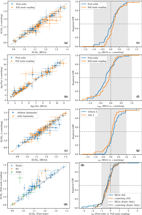
Figure 4. Various pairwise comparisons, as in Figure 3. In parts (a)–(d) (left column) we show direct comparison between inferred quantities, and in parts (e)–(h) (right column) we show the empirical cumulative distributions of the normalized differences, per Equation (10).
Download figure:
Standard image High-resolution imageOnce a full accounting for mixed-mode coupling is introduced, the two methods do disagree on the inferred masses, while the discrepancies in the inferred ages are no longer significant at the 3σ level. Generally speaking, we find that the use of a complete prescription for mode coupling results in slightly wider posterior distributions (and hence diminished effect sizes when normalized by the reported uncertainties), which may explain the loss of significance in the differences in the ages. However, the differences in the reported masses still suggests that the two surface-term treatments respond differently to extended descriptions of mode coupling. We have no good a priori explanation for this phenomenon.
4.3. Benchmark: Inclusion of Other Constraints
We now seek to compare the size of the systematic variations originating from different surface-term treatments with those arising from other methodological decisions in the modeling procedure. For example, we might introduce an additional contribution to the cost function,
where L is the stellar luminosity. For this exercise we restricted ourselves to the subset of our targets for which luminosities were available, either from their associated boutique modeling efforts (for the TESS targets) or from Gaia DR2 (Gaia Collaboration et al. 2018) for the Kepler and K2 targets. This excluded two K2 subgiants, δ Eri, and three Kepler subgiants from our sample. We show the results of this test in the seventh and eighth columns of Table 3, restricting ourselves to considering only cases where mode coupling is fully accounted for. Contrary to expectations, we see that the introduction of the luminosity constraint does not significantly modify the estimates of the stellar properties under our consideration when using the BG14 surface correction; while the effects are relatively larger for the -matching algorithm (yielding smaller p-values), they are nonetheless also not significant at the 3σ level. We examine this more closely in the next subsection.
The discrepancy between how these two surface-term treatments respond to the introduction of the luminosity constraint can be better examined by comparing them directly to each other, fully accounting for mode coupling, which we show in the sixth column of Table 3. We find that the presence of the luminosity constraint brings the two surface-term treatments into closer agreement with each other, resolving the statistical tension between them from the previous section. Specifically, we show the stellar masses and the distribution of their normalized differences in Figures 4(c) and (g): we see that the introduction of the luminosity constraint brings the inferred values from both methods closer to equality, on average. Since the generalized BG14 masses (i.e., with full mode coupling) are also less changed upon the introduction of the luminosity constraint, this suggests that the differences in behavior between the two surface-term treatments discussed in the previous section may ultimately be a result of nonparametric methods being potentially too flexible (yielding false positives) in this phase of evolution. Conversely, this might also imply that the generalized BG14 correction may provide more robust parameter estimates for subgiants than -matching, in the absence of luminosity measurements.
4.4. Survey and Single-target Systematics
Given that we have included subgiants from surveys of varying data quality, one might question whether or not those systematic differences that we have found have been driven by outliers, rather than being statistically representative of subgiants in general. For our most significantly discrepant set of pairwise differences—stellar masses under different treatments of mode coupling (Figure 3(a))—we see that there are a few potential outliers in our sample. Subdividing the BG14 masses by originating survey (Figure 4(d)), we find that the most extreme deviations from equality are indeed from K2 and TESS, which (per our previous discussion) are of somewhat degraded quality compared to nominal Kepler photometry. However, the distributions of normalized differences (Figure 4(h)) are not substantially modified when we restrict our attention to only Kepler subgiants; repeating the two-tailed t-test with only the Kepler subsample yields p = 5.612 × 10⁻⁵ for the BG14 correction and p = 0.0014 for -matching, which are both significant at the 3σ level. In general we find that our findings in the preceding subsections are not substantively changed when limited in scope to the Kepler subsample.
We now examine in detail the most discrepant data point in Figure 4(d), which turns out to be the TESS subgiant TOI-197. Unusually within our sample, but like most other TESS subgiants, only a very small number of modes (eight in total with two more uncertain) were identified for this star. Given this paucity of data, misidentification of g-modes (as described in Ong & Basu 2020) may yield significant systematic error. Moreover, TOI-197 is in such a state of evolution that the spacing of dipole g-modes near  is comparable to that of p-modes, rather than being significantly larger or smaller. In this regime, a complicated, highly nonasymptotic mixed-mode pattern is obtained rather than individually identifiable avoided crossings. As such, extremely fine temporal and parameter sampling (i.e., "boutique" modeling) should be necessary a priori. Fortunately, Huber et al. (2019) have already performed just such a boutique seismic characterization of TOI-197. In order to account for other sources of systematic methodological variability (as described in the next subsection), they employed multiple combinations of parameter search techniques (both optimization-based and grid-based), stellar evolution codes, inputs to stellar evolution (e.g., chemical mixture), and input physics. We may therefore assume that their parameter estimates are generally robust.
We show in Figure 5 a comparison of the posterior distributions obtained using various surface-term treatments (showing the contours of the first few standard quantiles with the solid colored curves), in comparison with the parameter estimates and reported uncertainties of Huber et al. (2019), shown with red lines and shaded intervals. We compare the posterior distributions for the BG14 correction under different treatments of mode coupling, with and without the inclusion of the luminosity constraint. We see that when mode coupling is only included to first order, the resulting parameter estimates are in tension with Huber et al. (2019), while the inclusion of the luminosity constraint does not tighten the posterior distribution. On the contrary, the posterior distribution is broadened, and develops a lobe in the direction of the nominal values from Huber et al. (2019); this is most visible in the mass–age and radius–age joint distributions. In the bottom left panel of Figure 5, we also show with the gray points the values of the mass–helium Sobol-sequence samples underlying the grid; this shows that the peak of the joint distribution is much further away from the nominal values of Huber et al. (2019) than can be explained solely by insufficiently dense sampling of the grid parameters. On the other hand, when mode coupling is fully accounted for, the posterior distribution is, while broad, nonetheless consistent with the boutique modeling estimate from Huber et al. (2019). The introduction of the luminosity constraint then significantly tightens the posterior distribution.
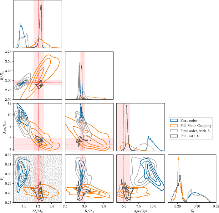
Figure 5. Corner plot for TOI-197, showing the 1σ, 2σ, and 3σ contours of the joint posterior distributions for different combinations of mode coupling treatment and spectroscopic constraints; the marginal probability density functions are shown on the diagonals. We show with red dashed lines and shaded intervals the literature values and uncertainties for the mass, radius, and age (as obtained from boutique modeling in Huber et al. 2019). In the bottom left panel, we show with the gray points the Sobol-sampled values of M and Y0 underlying the grid.
Download figure:
Standard image High-resolution imageTaken together, these are suggestive of the following interpretation: when fully accounting for mode coupling in the BG14 correction, the best-fitting region of parameter space sampled by the grid is in good agreement with the luminosity constraint. The luminosity likelihood function takes a maximum value near those of the other constraints, resulting in a considerably tighter posterior distribution when they are combined. Conversely, the best-fitting region in our grid under the first-order BG14 correction is in tension with the luminosity constraint. Moreover, the best-fitting models there lie in a local minimum in the cost-function landscape, which is sufficiently deep to interfere with the luminosity constraint.
Since qualitatively more correct estimates are returned from the full treatment of mode coupling, we find it unlikely that the difference between it and the first-order treatment are solely a result of poor data quality or grid artifacts. It is true that grid searches using an undersampled grid in combination with a paucity of mode frequencies are susceptible to spurious local minima, particularly when the characteristic avoided-crossing pattern (e.g., Bedding 2012) or reliable g-mode identification (e.g., Ong & Basu 2020) are not available. However, this affects both treatments of mode coupling, and therefore cannot adequately explain the differences between them. Rather, as we showed in Paper I, first-order approximations to mode coupling become increasingly unreliable (for a fixed relative size of the surface term) as stars evolve to lower values of Δν. Consequently, an incomplete treatment of mode coupling will cause any local minimum in the cost function to lie in a different region of parameter space, compared to when a correct accounting of mode coupling is used; the distance between the two will be larger for more evolved subgiants.
As discussed earlier, luminosity measurements are in principle capable of resolving the degeneracy between stellar mass and initial helium abundance. However, we see from Figure 5 that in the case of TOI-197, the treatment of mixed-mode coupling has a more significant effect on the estimated initial helium abundance than does the presence or absence of a luminosity constraint. Our above discussion in turn implies that accurate estimation of the initial helium abundance from subgiants that are at least as evolved as TOI-197 (i.e., Δν ≲ 30 μHz) will require full mode-coupling computations to be performed when correcting for the surface term.
4.5. Benchmark: Other Methodological Variations
Finally, we examine methodological variability induced by differences in how the stellar models underlying the grid itself were constructed. For this purpose we use the stellar properties as estimated by Li et al. (2020a). Unlike the one used here, the model grid used in that work uses a fixed value of the mixing length parameter, a different chemical mixture (Asplund et al. 2009), a different sampling scheme (even-tempered uniform sampling rather than Sobol sequences), and a fixed metallicity–helium relation, and does not account for mass-dependent core overshoot. Consequently, we would expect offsets in the inferred ages and masses returned by both of these modeling pipelines, even adopting identical choices in the surface-term correction. To ensure at least some consistency, we adopt the same set of constraints: the spectroscopic observables Teff and [Fe/H], and the individual mode frequencies under the BG14 surface correction, taken to only first order in the mixed-mode coupling.
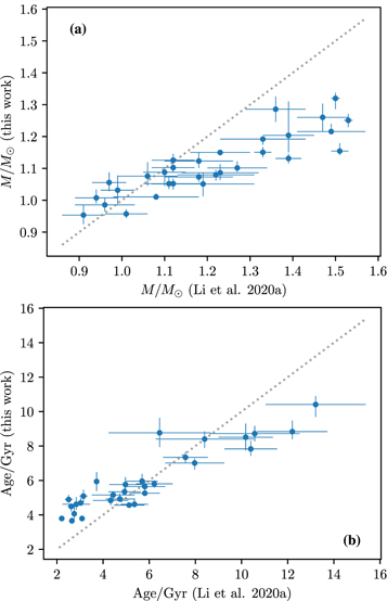
We show the results of these tests in the final column of Table 3. Unfortunately, Li et al. (2020a) make no attempt to infer the initial helium abundances of their sample; the grid used for these estimates assumes an intrinsic metallicity–helium relation, and so cannot meaningfully make such inferences. As such, we are unable to perform a comparison of this kind for Y0. We find that the differences in the inferred masses between our two pipelines are statistically significant; we show a direct comparison of the two in Figure 6(a). Note that while the absolute systematic differences are potentially larger than some of the effects we have seen in the previous comparisons in Figures 3 and 4, the errors reported by the grid of Li et al. (2020a) are significantly larger than those from our grid, owing to their much coarser grid sampling and less complete coverage of parameter space. Consequently, under the t-tests we have conducted, which operate on quantities normalized by the reported uncertainties, these differences are only significant at the 3σ level. This can also be seen in a similar comparison of the inferred stellar ages (Figure 6(b)), where likewise large systematic differences in the inferred ages are also seen but are not significant at the 3σ level.
Figure 6. Comparison of stellar masses (a) and ages (b) estimated from our grid vs. those from the model grid of Li et al. (2020a), using identical prescriptions for the surface term (BG14 to first order in mode coupling) and identical choices of spectroscopic constraints.
Download figure:
Standard image High-resolution image
5. Discussion and Conclusion
Ong et al. (2021a) showed that there exist qualitative differences in how stellar properties estimated from grid-based detailed seismic modeling respond to different methodological choices in correcting for the surface term. On one hand, estimates of the masses, radii, and ages of main-sequence stars appear largely insensitive to the choice of surface-term treatment, so long as one is performed (see Basu & Kinnane 2018; Compton et al. 2018; Nsamba et al. 2018). Any observed normal modes in these stars are all p-modes. On the other hand, estimates of these properties for a sample of red giants did appear to depend significantly on this methodological choice. The observed nonradial modes in this case are the most π-like of an otherwise g-mode-dominated eigenvalue spectrum. Neither of these results offered any useful methodological guidance for the analysis of subgiants, which lie in the intermediate regime where substantial nonradial coupling occurs between the outer p-mode and interior g-mode cavities. In order to extend that work to subgiants, we first had to generalize existing surface-term treatments to correctly account for mixed-mode coupling, which has hitherto been an open theoretical problem. This was done in Paper I.
In this work, we have instead considered how these constructions affect inferences of various fundamental stellar properties, for subgiants in particular. We have found that unlike main-sequence stars, but like the sample of red giants in Ong et al. (2021a), the inferred masses of stars in our subgiant sample do appear to depend systematically on which treatment of the surface term is used in the modeling procedure, and how mode coupling is handled in the process. A similar result is seen to hold for the stellar ages, although not at 3σ significance. On the other hand, while significant systematic differences in the inferred values of the initial helium abundance Y0 still exist, they appear considerably less sensitive to the choice of surface-term treatment for these subgiants than they were for the main-sequence sample of Ong et al. (2021a). Finally, parameter values estimated using the generalized BG14 correction appear to be somewhat more consistent with an additional luminosity constraint than those from -matching, once mode coupling is fully accounted for. Taken together, these are suggestive of intermediate behavior between main-sequence and red-giant oscillators, rather than there being a well-defined transition. However, the comparisons here have not completely explored the differences between these two extreme regimes. In particular, Ong et al. (2021a) found a qualitative difference between properties inferred using parametric surface-term corrections compared to nonparametric ones (via both the -matching algorithm and the method of separation ratios) on the red giant branch but not in main-sequence stars. A similar comparison would require generalizing the method of separation ratios to mixed modes, for which no theoretical construction is available at present.
As far as methodological guidance is concerned, we have found that fully accounting for mode coupling in the surface term results in at least different stellar masses compared to inferences made with first-order approximations to mode coupling. Fortunately, the absolute effects of changing the surface-term treatment appear to be still much smaller than those of changing the underlying physics used in constructing stellar models or the sampling strategy used in grid searches. Nonetheless, these surface-term methodological systematics are potentially significant at the 3σ level. Changing the prescription used for the surface term also appears to induce systematic offsets in the stellar age that are potentially comparable to, or larger than, those resulting from, e.g., the introduction of other global constraints, such as the luminosity.
Based on this, we recommend that generalizations of a similar kind to those we have described in Paper I be applied to prescriptions for surface-term corrections in general, if they are to be used for analyzing mixed modes in evolved stars (especially with Δν ≲ 30 μHz). Since many existing parametric surface-term corrections are either phenomenological or empirical in nature (e.g., Kjeldsen et al. 2008; Sonoi et al. 2015; Ball & Gizon 2017), the precise form of such generalizations may not be obvious. On the other hand, as described in Paper I, for more evolved stars these matrix methods may not yet be fully practicable, because of both numerical difficulties in evaluating the relevant coupling matrices and computational ones arising from the large rank of the matrices that are obtained for evolved stars. In those cases, restriction to the π-mode subsystem (as done in Ball et al. 2018; Ong et al. 2021a) might still ultimately be necessary, at least at present.
Finally, we must further qualify that these results, both here and in Ong et al. (2021a), are meant to be representative of multi-target grid searches rather than single-target boutique modeling. The multi-target strategy is typical of modeling pipelines intended for use with large-scale surveys, such as those currently being developed for the PLATO mission (see Cunha et al. 2021). It is more difficult to make general statements about how different surface-term treatments might affect the latter case, since such modeling work is by construction performed ad hoc. To the extent that these generalized treatments of the surface term may be more theoretically defensible for mixed modes, however, it seems reasonable to us that these results should also inform the decisions made in such boutique modeling.
The authors acknowledge the dedicated teams behind the Kepler and K2 missions, without whom this work would not have been possible. Short-cadence data were obtained through the Cycle 1–6 K2 Guest observer program. This work was partially supported by NASA K2 GO Award 80NSSC19K0102 and NASA TESS GO Award 80NSSC19K0374. We thank the Yale Center for Research Computing for guidance and use of the research computing infrastructure. Funding for the Stellar Astrophysics Centre is provided by The Danish National Research Foundation (Grant Agreement No.: DNRF106).
Software: NumPy (Harris et al. 2020), SciPy stack (Virtanen et al. 2020), AstroPy (Astropy Collaboration et al. 2013; Price-Whelan et al. 2018), Pandas (Reback et al. 2021), PBJam (Nielsen et al. 2021), diamonds (Corsaro & De Ridder 2014), mesa (Paxton et al. 2011, 2013, 2018), 4 gyre (Townsend & Teitler 2013).
Appendix
We provide the mode frequencies of all the stars in our K2 sample (including the main-sequence and red giant stars not explicitly modeled in this work) in Table 4.
Table 4. Mode Frequencies for Stars in the K2 Sample
| EPIC | l | ν/μHz | σν /μHz |
|---|---|---|---|
| 212478598 | 0 | 472.498571 | 0.009596 |
| 212478598 | 0 | 507.598629 | 0.019181 |
| 212478598 | 0 | 542.358328 | 0.008893 |
| 212478598 | 0 | 577.638506 | 0.012759 |
| 212478598 | 0 | 612.959501 | 0.012075 |
| 212478598 | 1 | 421.465770 | 0.010655 |
| 212478598 | 1 | 451.967692 | 0.008527 |
| 212478598 | 1 | 462.127731 | 0.012090 |
| 212478598 | 1 | 482.719768 | 0.035494 |
| 212478598 | 1 | 493.325932 | 0.012059 |
| ⋮ |
Only a portion of this table is shown here to demonstrate its form and content. A machine-readable version of the full table is available.
Download table as: DataTypeset image