


Abstract
We analyze the effect of polarized diffuse emission in the calibration of wide-beam millimeter-wave polarimeters, when using the Crab Nebula as a reference source for both polarized brightness and polarization angle. We show that, for CMB polarization experiments aiming at detecting B-mode in a scenario with a tensor to scalar ratio r ∼ 0.001, wide (a few degrees in diameter), precise ( ), high angular resolution (<FWHM) reference maps are needed to properly take into account the effects of diffuse polarized emission and avoid significant bias in the calibration.
Export citation and abstract BibTeX RIS
1. Introduction
Current and planned searches for the linear polarization of the CMB aim at the very faint rotational component produced during cosmic inflation, the so-called B-mode (see e.g., Kamionkowski & Kovetz 2016). This signature, produced by tensor perturbations originated in the very early universe, is extremely faint. Depending on the tensor to scalar ratio r, currently constrained to be r < 0.06 (see, e.g., BICEP2 Collaboration et al. 2018; Planck Collaboration et al. 2020; Tristram et al. 2021), the amplitude of such a signal can be smaller than a few nKCMB. Extreme sensitivity of the polarimetric survey is thus mandatory. In addition, such a signal is embedded in a much larger (a few μKCMB) irrotational (E-mode) polarized signal produced by scalar perturbations at recombination, as well as in a much larger polarized emission (E-mode and B-mode) generated by the interstellar medium in our Galaxy. This calls for extreme accuracy of the measurements.
Given the relative sizes of the signals, any unaccounted systematic effect (or physical process) producing B-mode or leaking a small fraction of the unpolarized signal or of the E-mode into B-mode would hamper this ambitious search for inflationary B-mode. B-mode of Galactic origin can be detected and marginalized exploiting the specific spectral signatures of synchrotron emission from interstellar electrons and thermal emission from interstellar dust.
Instrumental systematic effects must be carefully assessed and effective mitigation strategies must be put in place. Here we focus on one of the systematic effects, which is a small error Δα in the reference polarization direction of the polarimeter. This would produce a systematic bias in the B-mode (see, e.g., Pagano et al. 2009): the presence of such a systematic error biases the measured angular auto- and cross-power spectra  with respect to the original ones Cℓ
as follows:
with respect to the original ones Cℓ
as follows:
where T, E, and B stand for temperature anisotropy, E-mode polarization, and B-mode polarization respectively. From these equations one can see that, in order to detect B-mode corresponding to r ∼ 0.001, the error of the polarization direction reference Δα should be less than a few arcmin (see, e.g., Hu et al. 2003; O'Dea et al. 2007; Miller et al. 2009; Pagano et al. 2009).
A laboratory calibration at this level of accuracy is challenging and is not guaranteed to remain stable for the operation of the instrument in the field or during the space mission (see, e.g., Pajot et al. 2010).
One possibility is to exploit the fundamental symmetries of CMB polarization, since, in the standard scenario, the expectation values for the CMB temperature to B-mode correlation (〈TB〉) and E-mode to B-mode correlation (〈EB〉) vanish. So one could use Equation (1) for  and
and  to estimate Δα. This approach, however, would not allow us to probe nonstandard scenarios, including cosmic birefringence or the effects of parity violating physics (see, e.g., Carroll 1998; Lue et al. 1999; Gruppuso et al. 2011; Komatsu et al. 2011; Molinari et al. 2016; Planck Collaboration et al. 2016b).
A possible alternative way of measuring Δα using sky signals (Minami et al. 2019) exploits the fact that the rotation of the measured CMB polarization direction is due to both cosmic birefringence and reference direction error Δα, while the rotation of galactic dust polarization is due only to Δα.
The observation of extremely well characterized linearly polarized sources in the millimeter-wave sky would represent the most direct option for calibrating CMB polarimeters during their sky survey, in terms of the determination of the polarization angle and of the polarization degree. The agreement between the calibration resulting from such direct measurement and the calibration resulting from alternative methods would provide very strong evidence for the absence of systematic effects in both procedures. In this paper we analyze the problem of selecting the best polarized source in the millimeter-wave sky, with special attention to the problem of estimating contamination effects due to the polarized diffuse medium. The latter are especially important in forthcoming low angular resolution surveys, such as LSPE (The LSPE collaboration et al. 2021) and LiteBIRD (Hazumi et al. 2020).
The paper is organized as follows. In Section 2 we briefly summarize the properties of strong linearly polarized sources available in the millimeter-wave sky. In Section 3 we focus on the Crab Nebula and analyze the effect of diffuse foreground emission in wide-beam measurements targeting the Crab, using the forthcoming LSPE and LiteBIRD surveys as practical examples in Section 4. In Section 5 we discuss the results and summarize our conclusions.
2. Linearly Polarized Sources in the Millimeter-wave Sky
A good calibration source for CMB polarization surveys should be a bright, polarization pure, stable, compact source, at high Galactic latitudes. These are rare in the millimeter-wave sky. The two sources producing the strongest linearly polarized signal are Taurus-A in the northern hemisphere, and Centaurus-A in the southern hemisphere. One should also mention the edge of the Moon as a strong source of linear polarized radiation at millimeter waves (Poppi et al. 2002; QUIET Collaboration et al. 2011; Xu et al. 2020; Yang & Burgdorf 2020). However, the power emitted is very large compared to that of the target signals of sensitive multifrequency CMB surveys, and detector linearity issues represent a concern for the calibration. Also, in space-based surveys, the thermal stability of the instrument can be affected by the IR emission of the Moon. So we will not consider this source in the following.
The Crab Nebula (NGC 1952, Taurus-A) is a supernova remnant, with Galactic latitude ∼−5°, emitting strong synchrotron radiation up to very high frequencies. At millimeter and submillimeter wavelengths, it is the brightest extra-solar source in the sky featuring a high degree of linear polarization (with a polarized flux ∼14 Jy at 100 GHz; Mayer et al. 1957; Allen & Barrett 1967; Johnston & Hobbs 1969; Matveenko & Conklin 1973; Flett & Henderson 1979; Aumont et al. 2010; Wiesemeyer et al. 2011). For this reason, Tau-A has been often considered as a polarization calibrator for precision cosmic microwave background (CMB) polarization surveys (Leitch et al. 2002; Barkats et al. 2005; Aumont et al. 2010; Macías-Pérez et al. 2010; Weiland et al. 2011; Naess et al. 2014; Polarbear Collaboration et al. 2014; Planck Collaboration et al. 2016a; Kusaka et al. 2018; Ritacco et al. 2018; Aumont et al. 2020).
Centaurus-A (Cen-A) is an active galactic nucleus and bright radio galaxy (see, e.g., Israel 1998). Its Galactic latitude is 19°. Its optical counterpart is the elliptical galaxy NGC5128, at a distance of 3.8 Mpc. The active nucleus of the galaxy produces a rich structure of jets and plumes, well studied by radio telescopes over several orders of magnitude of angular scales. The inner lobes of Cen-A are polarized, bright, and stable at millimeter waves, with a typical angular extension of 10'. The source has been observed with CMB polarimeters (see, e.g., Zemcov et al. 2010), but it is fainter than the Crab Nebula (with a polarized flux ∼2 Jy at 100 GHz). Other even fainter sources have been considered in Burke-Spolaor et al. (2009) for low-frequency measurements of CMB polarization.
A different approach relies on the polarization of diffuse Galactic emission, as mapped by previous experiments (see, e.g., Matsumura et al. 2010): while effective, this approach is not as direct as the measurement of a well characterized compact polarized source. The use of diffuse polarized emission, in fact, requires accurate a priori knowledge of the co-polar and cross-polar beams of the instrument, while in principle these can be measured directly if the polarized source is compact.
For these reasons, in the following we will focus on the Crab Nebula.
3. The Crab Nebula as a Polarization Calibrator and the Effect of Diffuse Emission
We have used multifrequency Stokes T, Q, and U maps from the Planck Legacy Archive 1 (Dupac 2015; Planck Collaboration et al. 2020) to estimate the polarized signal measured by a wide-beam experiment targeting the Crab Nebula. The Nebula has an optical size of the order of 5' × 5', while the beam size of CMB experiments aiming at large-scale polarization measurements can be wider (order of 5'–100' FWHM, depending on the experiment and wavelength). This means that the CMB polarimeter will detect polarized diffuse Galactic emission in addition to the polarized signal from the Crab Nebula. Since the Nebula will be diluted in the wide beam of the detector, while diffuse emission will fill it, the contribution of diffuse emission to the detected signal might be relevant.
Inspection of the 545 and 857 GHz intensity maps from the Planck mission confirms that the Crab Nebula lies on the same line of sight as a larger diffuse emission cloud, evident in Figure 1. The emission is much fainter at lower frequencies, pointing to interstellar dust emission.

Figure 1. Sky brightness measured by Planck in the regions surrounding the Crab Nebula. The maps are in Galactic coordinates, and the size of the black square centered on the Nebula is 1° × 1°. The panels are labeled with the observation frequency. The Crab Nebula, as seen in visible light, is 6' wide, so it is not resolved at the resolution of Planck detectors. The color scale has been tuned to saturate the Nebula and display the surrounding faint diffuse emission. It is evident that its brightness increases with frequency.
Download figure:
Standard image High-resolution imageIn principle, one might hope to separate the emission of the nebula from diffuse interstellar emission taking advantage of their different spectral signatures. However, as a matter of facts, the Crab Nebula is evident in the foreground component separated maps from the Planck survey, both in the synchrotron map and in the dust map, and the same is true for diffuse emission. Moreover, possible rotation of the polarization angle with frequency, due to the possible presence, along the line of sight, of dust clouds with different temperatures (see, e.g., Tassis & Pavlidou 2015) should be properly modeled. For this reason, we argue that the spectral-based separation is not trivial, and a specialized component separation pipeline will be needed. All this is beyond the scope of this paper and will be analyzed in a future paper. Here we focus on the analysis in the different frequency bands.
In order to estimate the relative contributions of the Crab Nebula and of diffuse polarized emission, we apply standard aperture photometry to the Planck maps for T, Q, and U, computing the measured flux Tm and the measured Stokes parameters of linear polarization Qm and Um . We consider a top-hat beam with increasing radius θ and solid angle ΩB = π θ2:


Since the maps follow the Healpix pixelization scheme (Górski et al. 2005) with pixel size parameter Nside, we have

where n is the number of pixels within the beam solid angle ΩB . The best estimate of the uncertainty on Fm is thus

where σi is the error of the measurement of T for pixel i as obtained from the pixel covariance information in the Planck Legacy Archive files. Similar equations hold for σ2(Qm ) and σ2(Um ). We report in Figure 2 the results of the flux estimates from Equation (2).
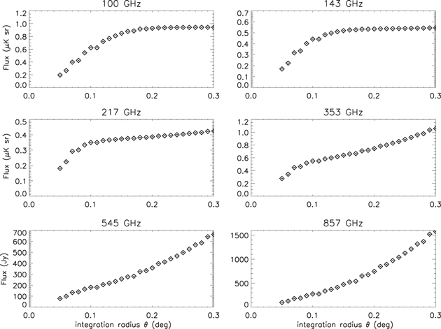
Figure 2. Aperture photometry of the flux Tm from the Crab Nebula (inner 5') and the surrounding regions, within a disk of radius θ. The panels are labeled with the observation frequency.
Download figure:
Standard image High-resolution imageThe error bars in the plots, as computed from Equation (6), are smaller than the size of the data points. At frequencies lower than 150 GHz the integration of the brightness converges, i.e., the flux from the Crab Nebula dominates over surrounding diffuse emission. At higher frequencies, however, the effect of diffuse emission is evident, even at distances from the center of the Crab as small as 0 15.
15.
Since interstellar emission is polarized, we expect a significant effect on the measured Qm and Um as well, especially at high frequencies. We can derive our estimates of the measured polarized signal and polarization direction, taking into account the effect of noise bias, as follows:
There is no polarization information from the Planck survey at frequencies of 545 and 857 GHz, so we limit our estimates to lower frequencies. The most important role of the polarized source is to provide a reference polarization direction ψ. Published measurements of ψ, limited to the Crab Nebula area, are consistent with a constant angle (Aumont et al. 2020)  in Galactic coordinates. There are two issues with this result: (a) this accuracy is insufficient for experiments targeting r ∼ 0.001, which require σ(ψ) ∼ a few arcmin; (b) when the measurement beam is wider than the Crab Nebula area, additional polarized emission from the surrounding diffuse medium will be detected and mix with that of the Nebula area, modifying ψm
with respect to
in Galactic coordinates. There are two issues with this result: (a) this accuracy is insufficient for experiments targeting r ∼ 0.001, which require σ(ψ) ∼ a few arcmin; (b) when the measurement beam is wider than the Crab Nebula area, additional polarized emission from the surrounding diffuse medium will be detected and mix with that of the Nebula area, modifying ψm
with respect to  . In order to investigate this effect, we use Planck data and Equation (7) integrating over increasing solid angles as before. The results are summarized in Figure 3.

Figure 3. Expected measured polarization angle ψm integrated over the Crab Nebula area (inner 5') and the surrounding regions, within a disk of radius θ. The panels are labeled with the observation frequency.
Download figure:
Standard image High-resolution imageFor a top-hat beam wider than 20' FWHM, at frequencies of the order of or higher than 143 GHz, ψm
differs from  by a significant amount, even 1° or more. For frequencies lower than 143 GHz the data do not provide strong evidence for a variation of ψm
, but the errors in the estimates are still large with respect to the few arcmin accuracy required for detecting r = 0.001.
by a significant amount, even 1° or more. For frequencies lower than 143 GHz the data do not provide strong evidence for a variation of ψm
, but the errors in the estimates are still large with respect to the few arcmin accuracy required for detecting r = 0.001.
A concern in this kind of estimate is the effect of noise bias (see, e.g., Simmons & Stewart 1985; Montier et al. 2015). In order to estimate the contribution of measurement noise, and to exclude bias effects in our simplistic estimators (Equation (7)), we carried out a simulation where the T, Q, and U Planck data in the Crab Nebula region have not been modified, while the Planck data in the surrounding region have been replaced by uncorrelated zero-average Gaussian noise realizations, with standard deviation mimicking the noise in the Planck data. We repeated the calculation of ψm
on these maps, and found that the trends visible at high frequencies disappear. At 353 GHz, the size of the fluctuations for ψm
is similar to the variations present in Figure 3 at small integration radii. Adding reasonable amounts of pixel-to-pixel correlated noise did not change the result. So we conclude that the detected deviation of ψm
from  for wide measurement beams is a genuine effect, due to diffuse polarized emission surrounding the Nebula. This is confirmed by visual inspection of the Q and U maps at 353 GHz, reported in Figure 4.

Figure 4. Stokes Q (left) and U (right) measured by Planck at 353 GHz in the region of the Crab Nebula. The maps are centered in the Nebula, in Galactic coordinates. The size of the black square centered on the Nebula is 1° × 1°.
Download figure:
Standard image High-resolution imageFrom Figure 4 it is evident that the Crab Nebula lays over a wide interstellar cloud with weakly positive Q and slightly negative U. In fact, if we exclude the Nebula area from our calculations of ψm
, integrating over a ring from θ = 01 to θ = 025, we obtain  ,
,  , and
, and  : these values are very far from
  .
.
We have also repeated the analysis using split Planck data (first half of the mission versus second half of the mission, and even versus odd rings). We find that significant differences in ψm are present, of the order of ∼10' at 100 GHz and ∼200' at 353 GHz.
The simple analysis carried out so far shows that if we want to use the Crab Nebula as an absolute polarization angle reference for wide-beam CMB polarization experiments (a) we cannot use the polarization of the Crab Nebula alone, since the contribution from the surrounding regions is relevant; (b) the accuracy of the Planck data is not sufficient to provide a reference ψm with ∼arcmin precision; (c) we need to carry out more accurate reference measurements over a wide solid angle (at least 1° in diameter), with sufficient sensitivity to measure the polarized signal of the diffuse cloud in addition to the polarized signal from the Nebula itself. Finally, we probably need to know the details of the beam shape of the instrument under calibration, since the effect of diffuse emission will be weighted by the beam response. We focus on this in the following section.
4. Beam Effects
For a polarization sensitive photometer (like, e.g., BICEP; BICEP2 & Keck Array Collaborations et al. 2015), the response to a polarized sky brightness described by the Stokes parameters T, Q, and U is given by:
where V is the measured signal,
n
is the boresight direction,  is the responsivity of the instrument, A is the collecting area;
  is the generic direction in the sky; the functions
  ,
,  , and
, and  represent the angular response (beam shape) of the instrument for unpolarized and polarized radiation; ψ is the angle between the main axis of the polarization sensitive photometer and the meridian of the sky coordinates;
  is the sky solid angle element.
For a Stokes polarimeter (like, e.g., SWIPE-LSPE; The LSPE collaboration et al. 2021 and LiteBIRD Hazumi et al. 2020), the response is given by:
where γ is the position angle of the half-wave plate (HWP) in the instrument reference frame. Here an ideal HWP is assumed, which does not modify the beam pattern.
In both cases, the beam calibration procedure is aimed at measuring the BT , BQ , and BU responses by mapping a source with known Stokes parameters Ts , Qs , and Us . If the source is compact (Ωs ≪ Ωbeam = ∫4π B*( n )dΩ), the integrals over the solid angle in Equations (8) and (9) reduce to products:
The three beam responses BT , BQ , and BU can then be measured by separating the corresponding components of the measured signal Wc by means of suitable modulation/demodulation techniques. This is the case of a ground calibration using a laboratory source, which can be rotated around the boresight to modulate Qs and Us (see, e.g., Masi et al. 2006; BICEP2 & Keck Array Collaborations et al. 2015). In the case of a fixed sky source, as being investigated here, the required modulation is obtained by repeating the scans on the source for different angles of the polarization sensitive polarimeter around its boresight (i.e., different values of ψ), or repeating the scans on the source for different angles of the HWP of the Stokes polarimeter (i.e., different values of γ). In sky calibration of BT is obtained from observation of planets. These, however, are unpolarized sources, and do not allow us to measure BQ and BU . So the usual procedure consists of a ground calibration of BT , BQ , and BU , and a sky calibration confirmation based on BT only. In the following we will assume that BT , BQ , and BU are known from the calibration procedure, and study how observations of a sky source with known ψs and Ps can provide a calibration of the polarization direction and of the polarimetric gain of the instrument.
The Crab Nebula is a compact object for most CMB polarimeters, but diffuse foreground emission, which is definitely extended, can be large enough to require the use of Equations (8) and (9), as suggested by the approximated top-hat beam analysis described in Section 3. Since available maps of diffuse foreground emission are noisy, the calibration will result in noisy estimates for the polarization angle reference and the polarimetric gain. Moreover, the strong emission of the Galactic plane, only 6° away from the Crab Nebula, might significantly contaminate the detected signals, due to the intermediate sidelobe response of BT , BQ , and BU . In the following we analyze in detail two specific examples of wide-beam polarimeters, using realistic beam assumptions.
For the purposes of this study we will neglect nonidealities in the polarimetric response of the instrument, and assume BT = BQ = BU = B. For single-mode optical systems we use a circular Airy profile averaged across the bandwidth of the instrument:


where νc is the center frequency of the receiver band, W is the bandwidth, J1 is the Bessel function of order 1, and D is the diameter of the optical aperture of the receiver. We model the presence of a forebaffle at angle θf as a decrease of B(θ) for angles larger than θf . We vary the amount of the decrease to investigate the effect of different levels of far sidelobes. Sample beams resulting from these assumptions are plotted in Figure 5.
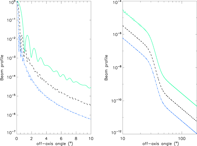
Figure 5. Left: sample beam profiles B(θ) used in this study (Equation (12)) for single-mode instruments. The parameters (νc , W/νc , D) are as follows: (33 GHz, 20%, 600 mm) for the continuous line, (100 GHz, 20%, 400 mm) for the dashed line, (340 GHz, 20%, 300 mm) for the dotted–dashed line. Right: far sidelobes of the beams used in this study. The ∼2 orders of magnitude decrease of the response at 30°–40° simulates the effect of a forebaffle.
Download figure:
Standard image High-resolution imageThese beams are assumed to be circular, while for the peripheral detectors, in a wide field-of-view array, significant ellipticity is usually measured (order of a few percent). Our circularity assumption is justified by the fact that in the following we will focus on Stokes polarimeters. Taking advantage of the polarization modulation induced by the rotation of the HWP, these polarimeters avoid the intensity to polarization leakage resulting from beam ellipticity in polarization sensitive photometers.
In the following we will repeat the analysis carried out in Section 3, including the effect of beam profile in the calculation of collected flux, as:


Here the boresight is assumed to be in ![$\left[{{\ell }}_{s},{b}_{s}\right]$](https://content.cld.iop.org/journals/0004-637X/921/1/34/revision1/apjac1860ieqn19.gif) , i.e., the coordinates of the target source (the Crab Nebula), and the distance of the generic sky element
, i.e., the coordinates of the target source (the Crab Nebula), and the distance of the generic sky element ![$\left[{\ell },b\right]$](https://content.cld.iop.org/journals/0004-637X/921/1/34/revision1/apjac1860ieqn20.gif) from the boresight is
from the boresight is

We study this beam-weighted aperture photometry for the measured polarization degree Pm and polarization angle ψm as a function of the integration radius θm , to check if the presence of diffuse polarized emission biases the results.
4.1. LSPE
The Large-scale Polarization Explorer (LSPE; The LSPE collaboration et al. 2021) aims at the detection of B-mode in the CMB at large angular scales and includes two synergic instruments. The Short Wavelength Instrument for the Polarization Explorer (SWIPE) is a balloon-borne Stokes polarimeter, while STRIP is a ground-based coherent correlation polarimeter.
The beams of SWIPE are determined by the optical aperture of the cryogenic telescope, which is 44 cm in diameter, and by the multimode feedhorns of the detector's array (Legg et al. 2016), which have the same aperture for the three measurement bands (145, 210, and 240 GHz). The beam FWHM is ∼85' for all bands. We use the beam responses of LSPE-SWIPE from Legg et al. (2016), modified to model also the additional sidelobe's reduction from the forebaffle: the beam response is further reduced by ∼20 dB for off-axis angles larger than 20°.
STRIP has single-mode receivers, and a large-aperture room-temperature cross-Dragone telescope, resulting in an FWHM of 20' and 10' for the 43 and 95 GHz bands respectively. We used Equations (12) as a first approximation for the beam responses of STRIP.
We compute the expected measured signals as a function of the integration radius following Equation (15). The results are reported in Figure 6. We avoided plotting error bars according to Equation (6), because the measured trends are due to intrinsic variation of the polarized sky signal, while the contribution of measurement noise is subdominant, especially for large integration radii.
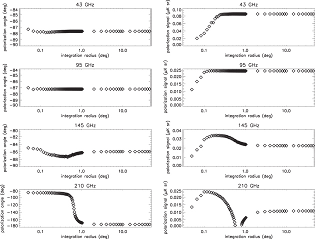
Figure 6. Beam-weighted aperture photometry of the polarization angle ψm (left) and polarized signal Pm (right) for the measurements of the LSPE polarimeters at 43, 95, 145, and 210 GHz (top to bottom rows), as a function of the integration radius around the Crab Nebula. The expected measured signals correspond to the largest integration radius, and differ from the signal from the Crab Nebula alone, which corresponds to the smallest integration radius.
Download figure:
Standard image High-resolution imageFrom the figure it is evident that the measured angle ψm
and the polarized signal Pm
converge for integration radii larger than ∼1°–2°. This means that the contribution from diffuse radiation is not negligible. As a matter of fact, ψm
and Pm
converge to values different from the values expected from the Crab Nebula alone. The difference is very important in the 210 and 240 GHz channels, where the signal from the Crab Nebula dominates for integration radii smaller than 03 while diffuse emission of interstellar dust in the Galactic plane takes over at larger angles, producing a ∼90° rotation of the polarization angle. Also at lower frequencies the effect of diffuse emission is not negligible:  at 145 GHz and at 43 GHz, while for the 95 GHz channel
  . Larger far sidelobe rejection from the forebaffle does not modify the results significantly. It is thus confirmed that in order to use the Crab Nebula as an accurate reference for the calibration of SWIPE, wide reference maps (a few degrees wide, with center on the Nebula position) would be needed.
4.2. LiteBIRD
LiteBIRD is the "Lite (Light) satellite for the studies of B-mode polarization and Inflation from cosmic background Radiation Detection," a JAXA-led space mission devoted to CMB polarization at large angular scales. LiteBIRD will produce ultrasensitive polarization maps of the full sky in 15 bands from 34 to 448 GHz (Hazumi et al. 2020). The 15 bands are distributed over three telescopes with different apertures. The resulting beam sizes range from 69' to 17' FWHM. In this case the instrument uses single-mode detectors, so we have used the beams described by Equation (12) as a first approximation of the LiteBIRD beams. The results for the aperture photometry described by Equation (15) are reported in Figure 7.

Figure 7. Beam-weighted aperture photometry of the polarization angle ψm (left) and polarized signal Pm (right) for the measurements of the LiteBIRD polarimeter at 40, 145, 195, and 337 GHz (rows from top to bottom), as a function of the integration radius around the Crab Nebula. The expected measured signals correspond to the largest integration radius, and differ from the signal from the Crab Nebula alone, which corresponds to the smallest integration radius.
Download figure:
Standard image High-resolution image
Here the measured angle ψm
and the polarized signal Pm
converge for integration radii larger than ∼05. ψm
and Pm
converge to values different from the values expected from the Crab Nebula alone. Due to the higher angular resolution, even at high frequencies we do not see the diffuse dust take-over seen for the LSPE-SWIPE 210 GHz channel. However, the differences are of the order of  . Again, it is confirmed that in order to use the Crab Nebula as an accurate reference for the calibration of LiteBIRD, wide reference maps (at least 15 wide, with center on the Nebula position) would be needed.
5. Discussion and Conclusions
In the previous sections we have demonstrated that the effect of diffuse polarized emission can bias the result of a polarimetric calibration of a wide-field polarimeter based on observations of the Crab Nebula. Two questions now arise:
(1) How precise and accurate should the reference polarization maps be to provide the required calibration accuracy?
(2) What is the requirement for the knowledge of the instrument beam response to attain a given calibration accuracy, which is based on convolutions of the beam responses with the polarized sky maps?
To answer the first question we have assumed that the Planck maps (Healpix pixelization with Nside = 2048) represent the real sky, in intensity and in polarization. We added 10,000 realizations of uncorrelated Gaussian noise to the values of T, Q, and U of each pixel, with a standard deviation of the noise per pixel of 10 μKCMB. The resulting distribution of the ψm angles has a standard deviation of less than 1' for the 40 GHz channel, and less than 3' for the higher frequency channels. This basically sets the requirement for the depth and accuracy of the reference maps: a very demanding requirement, especially for the highest frequency maps.
To answer the second question, we assumed again that the Planck maps represent the real sky, and simulated a couple of typical systematic errors in the beam map B, investigating their impact in the measurement of ψm and Pm .
The simplest systematic is an error in the solid angle of the beam. The typical measurement accuracy produces an error of the order of <0.5% on the solid angle (see, e.g., Planck Collaboration et al. 2014). We ran our convolutions and evaluated the convergence of ψm and Pm as a function of the beam FWHM in the case of a Gaussian beam (which is a good approximation of the main beam for single-mode systems). We found that a variation of the average measured ψm of the order of 1' is produced by a ∼1% variation of the FWHM. This means that standard beam measurements are sufficient in this respect.
In principle, for this kind of measurement, errors in the evaluation of the sidelobes can be as important as errors in the estimate of the FWHM. Sidelobe response measurements become increasingly difficult as the beam response declines with the off-axis angle. For the range of off-axis angles of interest here (a few to a few tens of degrees off-axis) we expect a measurement error of ∼0.1% to ∼1% of the beam response. This is mainly due to the difficulty of controlling systematic effects, due to the large size of the device under test, including the telescope and the surrounding structures, and the implied size of the compact range illuminator and the anechoic chamber. The difficulty is exacerbated by the need of testing the full instrument at cryogenic temperature. As an example, we have considered a 1% to 10% error in the amplitude of the first sidelobe of the beams used in Figure 7, where the angular response is already at the ∼1% level (see left panel in Figure 5). For a 1% increase of the first sidelobe, the resulting change of ψm is less than 1'. For a 10% increase of the first sidelobe, the change of ψm becomes (slightly) larger than 1' only in the 337 GHz channel. We do not claim that this example is representative of all possible systematic effects affecting beam measurements; however, it provides an indication of the required accuracy of side-lobe response determination.
In summary, we conclude that using the Crab Nebula as a reference for the calibration of future wide-beam CMB polarimeters, aiming at the measurement of B-mode with r ∼ 0.001, is challenging, due to the effects of polarized foreground emission in the surroundings of the nebula. The measurements require wide reference maps, with a precision of ∼20 μKCMB arcmin, over an area with a radius of a few degrees centered on the nebula. The preparation of such a set of maps requires a coordinated multi-instrument effort, including space-borne measurements at the high-frequency end of the frequency range of interest.
This work has been supported by the Italian Space Agency (ASI) through the contracts LSPE and LiteBIRD Phase-A, and by the National Institute for Nuclear Physics (INFN) through the CSN2 activity LSPE. The paper uses data obtained with the Planck satellite (http://www.esa.int/Planck), an ESA science mission with instruments and contributions directly funded by ESA Member States, NASA, and Canada. The data are maintained by the European Space Agency (ESA) at the the Planck Legacy Archive (https://wiki.cosmos.esa.int/planck-legacy-archive). We acknowledge the use of the HEALPix package (Górski et al. 2005).