


Abstract
Magnetohydrodynamic (MHD) turbulence is revealed to have scaling anisotropy based on structure function calculations. Recent studies on solar wind turbulence found that the scaling anisotropy disappears when removing large-scale field structures. This finding raises questions as to whether numerical MHD turbulences have large-scale field structures. How do these structures affect the scaling anisotropy therein? Here we investigate these questions with a driven compressible three-dimensional MHD turbulence. We introduce a new method to check how the random stationarity condition is satisfied. We find for the first time in the numerical MHD turbulence that the large-scale field structures destroy the random stationarity of the local fields and make samplings nonparallel to the instantaneous fields be calculated as apparent parallel samplings. This mixture makes statistical calculations show anisotropic scaling of the turbulence. When we select only the random stationary data intervals, the statistical results show an isotropic nature. We also find that among the large-scale field structures, one-third are tangential discontinuities (TDs), one-third are rotational discontinuities (RDs), and the rest are EDs (either TD or RD). These results show that the large-scale structures in the numerical MHD turbulence have important influence on the structure function analysis.
Export citation and abstract BibTeX RIS
1. Introduction
The measurement of the turbulence scaling index is important because the scaling index may provide clues as to the energy cascade mechanisms as well as the turbulence energy process such as the damping and heating (Goldstein et al. 1995; Tu & Marsch 1995; Biskamp 2003; Bruno & Carbone 2013; Howes & Nielson 2013). For the magnetohydrodynamic (MHD) turbulence, several energy cascade models are proposed, such as the ones by Kolmogorov (1941), Kraichnan (1965), Goldreich & Sridhar (1995), and Boldyrev (2006). The spectrum indices predicted by these models respectively are −5/3; −3/2, −2 (parallel); −5/3 (perpendicular); and −2(parallel), −3/2(perpendicular1), −5/3(perpendicular2), where parallel and perpendicular refer to mean fields. One can see that different models assume different energy cascade mechanisms and predict different scaling indices.
The measurement of the turbulence scaling index is not an easy task. It is a statistical analysis on a large number of measurements on turbulence variations. One needs to guarantee that the data are stationary and an ergodic random function of time. These conditions require that the local average of magnetic fields should not be sensitive to intervals for this average. If some intervals include large-amplitude variations, a random and time stationary condition would not be guaranteed and the accurate scaling measurement may not be obtained. The large-amplitude variations will lead to the nonstationary conditions preferring to appear at large scales, where the fluctuations are prone to experiencing violent variations. The large-amplitude variations will also make a mix of parallel and nonparallel samplings. The local magnetic field is usually computed by the average of the magnetic field vectors measured at two time instants or two space points (Cho & Vishniac 2000; Milano et al. 2001; Luo & Wu 2010; Pei et al. 2016; Yang et al. 2018a). If this average field direction is parallel to the sampling direction, this measurement is considered a parallel selection. However, this average field direction may not represent most of the instantaneous field directions, which results in some apparent nonparallel samplings to be considered parallel samplings. Under this circumstance, the constructed parallel spectral density is contaminated by nonparallel fluctuations. These features combine making the measurement of the parallel scaling very difficult (Wang et al. 2016).
Since large-scale coherent structures appear in both the solar wind turbulence and the simulated turbulence, one needs to study whether the large-scale structures have some influence on the parallel scaling measurement (Matthaeus & Goldstein 1986; Matthaeus & Velli 2011), and if yes, how to avoid the influence. Is there a limitation for the use of MHD turbulence of the structure function method that is widely used for evaluation of the scaling index in hydrodynamic (HD) turbulence? If large-scale coherent structures mix in MHD turbulent fields, one should consider making some improvements for the use of the structure function method to reject the influence of the large-scale structures.
The solar wind turbulence has been studied for several years and it has been found that coherent structures can have a large effect on the measurement of the turbulence scaling index (Horbury et al. 2012; Wang et al. 2014, 2015, 2016; Pei et al. 2016; Telloni et al. 2019; Carbone et al. 2020; Chhiber et al. 2020; Wu et al. 2020; Zhao et al. 2020). Recently, the influence of large-scale coherent structures on the scaling measurement was first noticed by Wu et al. (2020). Through an improvement of the structure function method, they found the isotropic scaling feature of the calculated structure functions, which only include the data intervals selected according to the criterion ϕ < 10° with ϕ being the angle between the two local mean magnetic fields averaged over the two adjacent halves of the data intervals.
For the numerical MHD turbulence, the problem of the influence of large-scale coherent structures on the scaling measurement has not yet been studied, although the scaling anisotropy has been reported in many numerical simulations (Matthaeus et al. 1996; Cho & Vishniac 2000; Maron & Goldreich 2001; Milano et al. 2001; Müller et al. 2003; Müller & Grappin 2005; Beresnyak & Lazarian 2009; Chen et al. 2011; Mallet et al. 2016; Yang et al. 2017a, 2018a). Cho & Vishniac (2000) introduced the structure function method to study the scaling nature and found the numerical MHD turbulence to be anisotropy. The local statistics adopted by Cho & Vishniac (2000) may suffer from some difficulties and conceptual problems as discussed by Matthaeus et al. (2012). The calculated second-order structure functions may mix with higher order moments as a stochastic coordinate system is established to get local parallel and perpendicular directions, which implies that the information that the locally oriented second-order structure functions contains may be different from that of the energy spectrum (Matthaeus et al. 2012). Chen et al. (2011) provided the measurement of the spectral scaling parallel to the local mean field in the reduced MHD simulations of turbulence, and showed that the parallel index is close to −2, supporting the model by Goldreich & Sridhar (1995). It should be noted that in these works they use the structure function method, which may have some limitations in the case of the influence of coherent structures. Since coherent structures are ubiquitous in numerical MHD turbulence (Maron & Goldreich 2001; Greco et al. 2008, 2009; Uritsky et al. 2010; Servidio et al. 2011; Zhdankin et al. 2012, 2014, 2015; Zhang et al. 2015; Yang et al. 2015, 2017a, 2017b, 2017c, 2018a), the influence of coherent structures, especially the large-scale ones, on the measurement of the scaling index by the use of structure function method should be studied in detail.
Although the large-scale structures' influence on the scaling measurement has been studied for solar wind turbulence, we still need to study this problem in the numerical MHD turbulence. There are some differences between the two turbulences. The origin of the large-scale structures may be different in these two turbulences. For the former, the large-scale structures may originate from the solar corona, while for the latter, the large-scale structures are generated locally and distributed homogeneously in the geometric space. The data measurement is also different in these two turbulences. For the former, the measurement is made by a spacecraft resulting in one-dimensional (1D) data, while for the latter, the measurement results in three-dimensional (3D) data. The data analysis on the numerical MHD turbulence may provide better insight into the turbulence nature than the 1D data observed in the solar wind turbulence.
Here we first investigate the limitation of the structure function method in the measurement of the scaling anisotropy in a numerical MHD turbulence and try to remove the influence of the large-scale structures on the estimated scaling index in the parallel-sampling case. The turbulence is produced by a numerical code with driven forces at large scales. We aim to guarantee that each selected interval is random stationary. To check how the parallel-sampling condition is satisfied, we introduce a new method to measure the geometrical distance between the magnetic field lines connecting, respectively, with the two separated points of the structure function and the geometrical line connecting these two separated points. We examine whether the local parallel samplings are along the magnetic field directions and whether the reconstructed parallel spectrum is contaminated by large-scale structures or nonparallel-sampling fluctuations. We also try to identify the nature of large-scale structures and evaluate the influence of these structures on the accuracy of the scaling measurement. This paper is organized as follows: In Section 2, we describe the setting of our numerical simulation. In Section 3, we present our numerical results, and in Section 4, we provide a brief conclusion and discussion.
2. Numerical Methods
The 3D compressible MHD model used in this paper was detailed in (Yang et al. 2017c, 2018b), and the governing equations read as follows:


with e = (1/2)ρ u 2 + p/(γ − 1) + (1/2) B 2 and j = ∇ × B corresponding to the total energy density and current density, respectively. Here, ρ is the mass density; p is the thermal pressure; u is the the velocity field; B = B 0 + b denotes the total magnetic field; t is time; γ = 5/3 is the adiabatic index; ν = 10−4 is the viscosity; and η = 10−4 is the magnetic resistivity. The large-scale mean field B 0 (=1.00) is imposed in the z direction.
Turbulence is driven by the large-scale random forces f 1 and f 2, which produce Alfvénic perturbations propagating antiparallel and parallel to magnetic field, respectively (Yang et al. 2017c, 2018b). f 1 and f 2 are isotropic in k space and are composed of 21 Fourier modes with wavenumber k ≤ 3.5 and the uniform-distributed random phase angle between [0, 2π]. The amplitude of each mode is a constant plus a small noise. Meanwhile, f 1 and f 2 are designed to be non-compressive, satisfying ∇ · f 1 = 0 and ∇ · f 2 = 0, respectively.
We consider periodic boundary conditions in a cube with a side length of 2π and a resolution defined by the number of grid points, which is 10243. We apply a third-order piecewise parabolic method to the reconstruction and an approximate Riemann solver of Harten–Lax–van Leer discontinuities to calculation of numerical fluxes. The constrained transport algorithm is employed to ensure a divergence-free state of the magnetic field.
After turbulent quantities reach a statistically quasi-stationary state, we conduct the analyses as shown in Section 3. The rms values for velocity and magnetic field are approximately 0.39 and 0.34, respectively; cross-helicity σc = 0.50, plasma beta β = 1.64, and averaged Alfvén speed 〈VA 〉 = 1.00.
The second-order structure function is computed by
where
U
could be either
B
or
u
,
l
is the position vector of points,
r
is separation vector between a pair of points, which are picked at random, N is the total number of pairs at θRB, r, and ϕ, and θRB is angle between
r
and the local mean magnetic field, and
B
l
.
B
l
is calculated as follows: first we divide the intervals between
l
+
r
and
l
into two halves with the same duration of
r
/2. Then, we compute the mean field of each half, marked as
B
l1 and
B
l2. Finally, the local mean magnetic field,
B
l
, is given by  (Wu et al. 2020). ϕ is the angle between
B
l1 and
B
l2. At certain ranges of θRB, r, and ϕ, most of the structure function values are the average of tens of thousands of pairs of points.
(Wu et al. 2020). ϕ is the angle between
B
l1 and
B
l2. At certain ranges of θRB, r, and ϕ, most of the structure function values are the average of tens of thousands of pairs of points.
Different from the previous calculations of the structure functions, in which the structure function is a function of θRB and r (Cho & Vishniac 2000; Luo & Wu 2010; Yang et al. 2018a), the introduction of ϕ into the current calculation of the structure functions is to ensure the randomly picked series of the magnetic field to be random stationary (Wu et al. 2020). As shown below, the constraint placed by ϕ can prevent the large-scale structures from the influence on the local parallel structure functions and the mixing of parallel and nonparallel samplings.
3. Simulation Results
To see the impact of ϕ on the spectral scaling, we only reserve those intervals with ϕ < ϕc in the calculation of the structure functions. ϕc is set as [10°,15°,20°,25°,...,90°]. The left panels of Figure 1 show the variations of the local parallel spectral index with ϕc . We adopt a linear fit on log-log scales to estimate the structure function's scaling index ζ. The spectral index α is obtained by the relation α = − ζ−1. The spectral index varies from −1.86 with ϕc = 90° to −1.64 with ϕc = 10° for the magnetic field and from −1.88 with ϕc = 90° to −1.77 with ϕc = 10° for the velocity. When ϕc is between 15° and 40°, the spectral index changes dramatically. When ϕc is ∼ <15°, the spectral index alters little. Based on these results, we assume that the intervals with ϕ < 10° have homogeneous background fields, which means that the local mean field direction represents the major instantaneous field directions, and that the intervals with ϕ ≥ 10° have nonhomogeneous background fields.
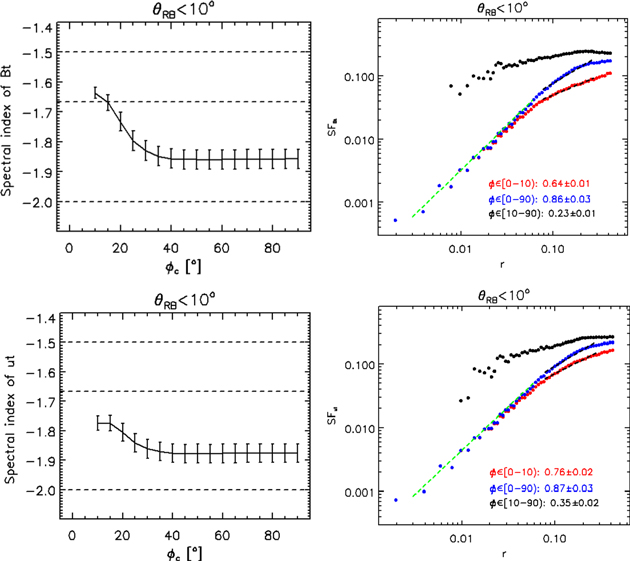
Figure 1. Results with different criteria of ϕc for the local parallel structure functions (θRB < 10°) of the magnetic field (top panels) and the velocity (bottom panels). (Left panels) Spectral index with respect to ϕ bins when the intervals with ϕ < ϕc in each bin are accumulated. (Right panels) Structure functions when the intervals with ϕ in the given bin are accumulated. The unit of the horizontal ordinate is in terms of the box size. The black dashed lines show a linear fit to the local parallel structure functions on log-log scales, which provides the scaling indices as well as their uncertainties marked in the corresponding colors.
Download figure:
Standard image High-resolution imageThe right panels of Figure 1 present the magnetic-trace and velocity-trace local parallel structure functions computed by the accumulated intervals under the conditions of ϕ < 10° (red dots), ϕ < 90° (blue dots), as well as 10° ≤ ϕ < 90° (black dots). In the range of 0.49 ≤ r ≤ 1.72, the local parallel structure functions show power laws, and this range is considered to be within the inertial range of the driven turbulence. At each scale, the reserved intervals with ϕ < 10° result in much smaller structure functions than those induced by the rejected intervals with 10° ≤ ϕ < 90°. The comparison of the structure functions with ϕ < 10° to those with ϕ < 90° reveals that the removed intervals conspicuously reduce the power of the structure functions at the large scales.
It can be noted that the local parallel structure functions display a long dissipation range, which illustrates that the code is highly diffusive due to the use of the Godunov-based method. By a linear fit to the local parallel structure functions on log-log scales, which is shown as the green lines in Figure 1, it is found that the local parallel structure functions at the dissipation regime have a power-law scaling with the index of ~1.42 for the magnetic field and ∼1.37 for the velocity. These power-law indices are smaller than those in the kinetic ranges of the solar wind turbulence (Chen et al. 2010; Duan et al. 2021), which may be due to the used two-point structure functions. As indicated by these authors (Cho 2019; Wang et al. 2020), five-point structure functions seem more appropriate for studying scaling laws at the dissipation regime.
Figure 2 shows the spectral indices of the magnetic field and the velocity as a function of θRB with ϕ < 90° (left panels) and ϕ < 10° (right panels). It can be seen that when no restriction by ϕ is placed, anisotropy exists and manifests itself in the spectral index for the fluctuations in the two driven fields. However, with the homogeneous local mean field, which is fulfilled by the criterion of ϕ < 10°, the driven turbulence displays the isotropic scaling feature. Like the solar wind turbulence (Wu et al. 2020), the removed intervals with 10° ≤ ϕ < 90° have a slight effect on the perpendicular scaling.
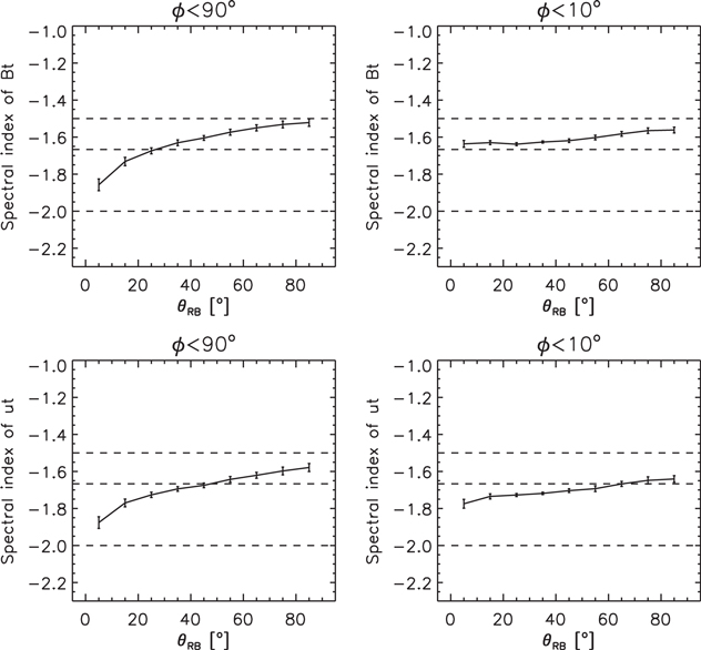
Figure 2. Spectral indices of the magnetic field (top panels) and the velocity (bottom panels) as a function of θRB with ϕ < 90° (left panels) and ϕ < 10° (right panels).
Download figure:
Standard image High-resolution imageFigure 3 presents the column-normalized 2D joint probability density function (PDF) of the interval number, which is plotted as follows: in each pixel of ϕ and r, there are N(r, ϕ) of intervals. At each scale r, we pick out the maximal value of the interval number,  . The column-normalized distribution of the interval number in Figure 3 is obtained by
  .
.
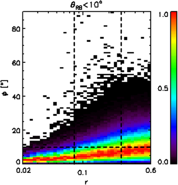
Figure 3. Column-normalized 2D joint PDF of the interval number on the ϕ−r plane for the local parallel intervals with θRB < 10°. The horizontal dashed line marks the criterion of ϕc = 10°, and the two vertical dashed lines bound the range used for the fitting analysis. The unit of the horizontal ordinate is in terms of the box size.
Download figure:
Standard image High-resolution imageWe can see from Figure 3 that with the scale r increasing, the angle ϕ of the pixels in red show that the maximum number in the pixel column at r is increasing. This figure is made under the condition θRB < 10°, which is generally considered as a condition for the selection of local parallel intervals. The data intervals with ϕ > 10° contain large variations in violation with the random stationary condition. These intervals cannot guarantee that the instantaneous field directions are parallel with the sampling directions. Meanwhile, these intervals have fluctuations with large amplitudes on large scales and make the second-order structure function and power spectrum power spectrum have steeper slopes with scale. To guarantee that most of the selected intervals meet the random stationary condition, one needs to add the selection condition ϕ < 10° in addition to the condition θRB < 10°.
To validate our assumption that the intervals with ϕ < 10° are with the homogeneous local mean fields, while the intervals with ϕ ≥ 10° are with the nonhomogeneous local mean fields, Figure 4 provides the typical geometry of two points sampled to calculate the local parallel structure functions with ϕ < 10° and ϕ > 10°. It can be seen that under the constraint imposed by ϕ < 10°, the sampling direction shown by the black line is nearly along the magnetic field direction across the sampled points, and the local mean field direction represents the major instantaneous field directions, indicating that the homogeneous local mean fields are satisfied. The sampling can achieve parallel measurement.
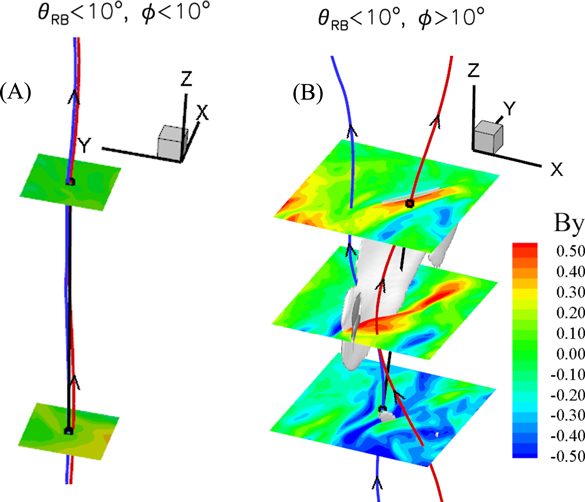
Figure 4. 3D geometry of two points sampled to calculate the local parallel structure functions (θRB < 10°) with ϕ < 10° (panel A) and ϕ > 10° (panel B). The two black cycles mark the positions of the two points, the black lines denote the separation vectors of the two points, the red line represents the magnetic field line across the upper points, and the blue line is the magnetic field line across the lower points. The color of the slices shows the distribution of the magnetic field component, and the white surfaces on panel B denote the isosurface where TVI = 7.
Download figure:
Standard image High-resolution imageHowever, the removed intervals with ϕ > 10° display a greatly different picture as shown in panel B of Figure 4. On the one hand, the directions of the field lines across the two sampled points have large separations, and the field line directions along the sampling path vary considerably. Therefore, the sampling direction cannot represent the major instantaneous field directions, and the sampling mixes the parallel-sampling and nonparallel-sampling fluctuations. On the other hand, the sampling passes through the discontinuity-like structures, which are marked by the isosurface of large normalized total variance of increments (TVI). TVI, as an indicator of intermittency (Greco et al. 2008; Zhang et al. 2015; Yang et al. 2017b, 2018a), is defined as

where
The partial derivative about x is computed as

with δx being the grid distance, Bβ denotes the corresponding component of the magnetic field, and w(=3) is the width.
The comparison between panel A and panel B of Figure 4 shows that the requirement of the homogeneous local mean fields successfully keeps the structures and the nonparallel-sampling fluctuations from mixing with the parallel-sampling fluctuations. The true parallel sampling yields the parallel spectra approaching more to a −5/3 scaling than a −2 scaling.
To analyze the nature of the structures that are excluded from the parallel measurement, we sample the variation of the plasma parameters and magnetic field across the isosurface of the TVI, and perform the minimum variance analysis (MVA; Sonnerup & Cahill 1967) of the magnetic field to find its maximum variance direction (l), its intermediate variance direction (m), and its minimum variance direction (n), and finally get the Alfvén velocity (VAl, VAm, VAn) as well as the plasma velocity (Vl, Vm, Vn) along these directions. Figure 5 presents one example of the structures, from which it can be seen that the large jumps in the Alfvén velocity and the plasma velocity mainly occur along their own l directions, while their n components over the entire sampling are close to 0. Meanwhile, across the interface of the structure, the total pressure Ptot exhibits a relatively constant trend, and both the magnetic pressure Pmag and the thermal pressure Pth have large jumps. These corroborate that this event is a tangential discontinuity (TD).

Figure 5. Profiles of the magnetic pressure Pmag, the thermal pressure Pth, the total pressure Ptot, the Alfvén velocity (VA shown as black lines), the plasma velocity (V shown as red lines), the density ρ, and the TVI across the isosurface of the TVI shown in Figure 4. The l−m−n coordinates are yielded from MVA on VA and V. The vertical dashed line marks the interface of the intermittency.
Download figure:
Standard image High-resolution imageBased on the MVA results, all of the eliminated structures are classified into four groups, according to the method defined by Smith (1973). This method of identifying the type of intermittency requires two parameters P1 = ∣Bn ∣/BL and P2 =δ∣ B ∣/BL , with Bn being the n component of the magnetic field B and BL being larger than the l component of the magnetic field. The events with P1 < 0.2 and P2 > 0.2 are identified as TD, the events with P1 > 0.4 and P2 < 0.2 are identified as rotational discontinuity (RD), the events with P1 < 0.4 and P2 < 0.2 are identified as ED (either TD or RD), and the events with P1 > 0.2 and P2 > 0.2 are identified as ND (neither TD nor RD). Among the structures, we find that about one-third is TD, one-third is RD, and the other third is ED.
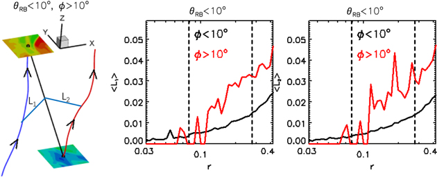
To quantify the mix of nonparallel and parallel samplings, we measure the geometrical distance L1 and L2 between the field lines and the geometrical line connecting the two points of the structure functions. As shown in the left panel of Figure 6, L1 and L2 are perpendicular to the sampled parallel interval (the black line) and intersect with the field lines passing over the two points. To quantify L1 and L2, we first take about 20 points, which are uniformly spaced along the sampled parallel intervals, and then get about 20 L1 and L2 associated with these 20 points. Finally, we average L1 and L2 according to the length of the intervals (that is the scale r), and plot the variation of the mean L1 and L2 with the scale r in the middle and right panels. The smaller 〈L1〉 and 〈L2〉 are, the more the sampling directions approach the true parallel directions.
Figure 6. Quantification of the mixing of nonparallel and parallel samplings. (Left panel) The same format as that of Figure 4, with L1 and L2 denoting the length of the lines perpendicular to the sampling direction (black line) and intersecting with the field lines passing over the two sampled points (black cycles). (Middle and right panels) Variation of the mean L1 and L2 with the scale r for the homogeneous magnetic field series (ϕ < 10°, black lines) and the nonhomogeneous magnetic field series (ϕ > 10°, red lines). The two vertical dashed lines bound the fitting range. The unit of the horizontal and vertical ordinates is in terms of the box size.
Download figure:
Standard image High-resolution image
From Figure 6, it is found that 〈L1〉 and 〈L2〉 obtained from the intervals with the nonhomogeneous magnetic field series (ϕ > 10°) are larger than those from the intervals with the homogeneous magnetic field series (ϕ < 10°). At the upper end of the fitting range, marked by the right dashed line in the middle and right panels, 〈L1〉 and 〈L2〉 are about 12% of r for the nonhomogeneous magnetic field series, while they are only about 5% of r for the homogeneous magnetic field series. With the scale r decreasing, 〈L1〉 and 〈L2〉 from the intervals with the homogeneous magnetic field series become very small, meaning that the parallel measurement is satisfied.
4. Summary and Discussion
We perform a data analysis on the numerical MHD turbulence with the method of structure function, which is proposed by Cho & Vishniac (2000) to show the anisotropic scaling of the numerical MHD turbulence. We find for the first time that the local mean direction may not represent the major instantaneous field directions and the second-order structure functions are influenced by the large-scale field structures if some of the data series used for the data analysis are not random stationary based on an easy criterion. When these data series are removed, the analysis results show the isotropic scaling with about a −5/3 power-law index, but not the anisotropic scaling. We also identify the nature of these large-scale structures and measure the field line divergence appearing in the structure function analysis. These results may help evaluate the limitation of the use of the original structure function method in the MHD turbulence created by numerical simulation and in understanding the influence of the large-scale structures both in the numerical MHD turbulence and the solar wind turbulence.
In the following we provide more detailed descriptions of our results. To guarantee the random and the random stationarity, we select the data series with the local mean field fulfilling the criterion that ϕ < 10° with ϕ being the angle between the two local mean magnetic fields as averaged over the two halves divided from each the sampling intervals. We find that the parallel structure functions of both the magnetic field and the velocity approach 0.67 scaling rather than 1.00 scaling with no constraint on ϕ. The requirement of the random stationarity of the local mean field prevents the large-scale structures and the nonparallel-sampling fluctuations from mixing with the data sets selected for the parallel case. However, the requirement of the random stationary field series has nearly no effect on the scaling of the perpendicular structure functions with an index of about 0.67, which is the same as the parallel structure function scaling displaying the isotropic feature. Among the removed large-scale structures with ϕ > 10° for the parallel case with θRB < 10°, about one-third are identified as TDs, one-third as RDs, and the rest as EDs.
For the parallel-sampling intervals, we measure the geometrical distance between the magnetic field lines, respectively, passing through points A and B of any structure functions and the geometrical line connecting A and B. When the sampled magnetic field series is random stationary, both magnetic field lines from A and B coincide with the geometrical AB line. Otherwise, the two field lines and the AB line are separated form each other at a large distance. Thus, parallel sampling is not guaranteed and some variations from large perpendicular structures are mixed into the parallel case, resulting in its steeper spectral slope.
The structure function analysis is widely used in numerical MHD turbulence to study the turbulence anisotropy (Cho & Vishniac 2000; Maron & Goldreich 2001; Müller et al. 2003; Beresnyak & Lazarian 2009; Chen et al. 2011; Mallet et al. 2016; Yang et al. 2018a). It is found that the parallel-sampling second-order structure functions have a 1.00 scaling, with the perpendicular ones being a 0.67 scaling. These anisotropy results are different from the isotropic nature of the structure functions calculated with only homogeneous intervals shown in this work. We present here an easy way to check if the anisotropic nature resulting from the structure function analysis is influenced by the nonhomogeneous intervals determined by some large-scale structures possibly existing in the numerical MHD turbulence.
This work also helps us further understand the influence of the large-scale structures on the solar wind turbulence proposed by Wu et al. (2020), who performed a data analysis based on the observations by the spacecraft WIND. These 1D data sets provide little information across the geometric line connecting both of the two separate points, A and B, defined by the structure function method. One cannot directly identify the nature of the structures that influence the structure function analysis. Here we use the numerical MHD turbulence to identify the coherent structures as TDs, RDs, and EDs. Also due to the limitation of the observation data, Wu et al. (2020) did not demonstrate whether the parallel-sampling direction is along the field direction in the parallel case. Here we show that only in the random and homogeneous condition, the parallel direction, the field line direction, and the direction of the geometric line connecting the two separate points are almost near to each other and the parallel-sampling condition is guaranteed.
This work is supported by the National Natural Science Foundation of China under contract Nos. 41974171, 41974198, 41874199, 41874200, 41731067, 41774157, 41774183, and 41861134033. The work was carried out at National Supercomputer Center in Tianjin, China, and the calculations were performed on TianHe-1 (A). Honghong Wu is also supported by the China Postdoctoral Science Foundation (2020M680204 and BX2021006).