


Abstract
A newly born millisecond magnetar is thought to be the central engine of some gamma-ray bursts (GRBs), especially those that present long-lasting X-ray plateau emissions. By solving the field equations, we find that when the rotational speed of the magnetar is approaching the breakup limit, its radius R and moment of inertia I undergo an obvious evolution as the magnetar spins down. Meanwhile, the values of R and I sensitively depend on the adoption of a neutron star (NS) equation of state (EoS) and the NS baryonic mass. With different EoSs and baryonic mass considered, the magnetic dipole radiation luminosity (Ldip) could be variant within one to two orders of magnitude. We thus suggest that when using the X-ray plateau data of GRBs to diagnose the properties of the nascent NSs, EoS and NS mass information should be invoked as simultaneously constrained parameters. On the other hand, due to the evolution of R and I, the temporal behavior of Ldip becomes more complicated. For instance, if the spin-down process is dominated by gravitational wave emission due to the NS asymmetry caused by magnetic field distortion ( ), the segment Ldip ∝ t0 could be followed by Ldip ∝ t−γ with γ larger than 3. This case could naturally interpret the so-called internal X-ray plateau feature shown in some GRB afterglows, which means the sharp decay following the plateau unnecessarily corresponds to the collapse of the NS. This may explain why some internal X-ray plateaus are followed by late-time central engine activity, manifested through flares and second shallow plateaus.
Export citation and abstract BibTeX RIS
1. Introduction
With the successful launch of the Neil Gehrels Swift Observatory (Gehrels et al. 2004), early-time afterglows for gamma-ray bursts (GRBs) have been revealed. They are important for unveiling the open questions for GRB physics, such as their progenitors and central engines (see Zhang 2018, for a review). Observationally, a good fraction of the X-ray light curves of (long and short) GRBs have been discovered to show a long-lasting plateau feature. Such a feature seems to be consistent with the prediction of a millisecond magnetar (namely, rapidly spinning, strongly magnetized neutron star (NS)) engine, which is thought to have formed from a violent event such as the massive star collapse (for long GRBs) or double NS merger (for short GRBs) (Paczynski 1986; Eichler et al. 1989; Usov 1992; Woosley 1993; Thompson 1994; Dai & Lu 1998a, 1998b; MacFadyen & Woosley 1999; Zhang & Mészáros 2001; Metzger et al. 2008; Zhang 2011).
The energy reservoir of a newly born millisecond magnetar is the total rotational energy, which could be estimated as

where I is the moment of inertia and Ω = 2π/P is the angular frequency of the nascent NS. In principle, during the spin-down process, the nascent magnetar loses its rotational energy via both magnetic dipole radiation and gravitational wave (GW) emission, so that the spin-down law can be written as (Shapiro & Teukolsky 1983; Zhang & Mészáros 2001)
Bp
is the dipolar field strength at the magnetic poles on the NS surface. R and  are the radius and ellipticity of the NS, respectively. Depending on the NS properties, such as the values of Bp
and , the spin-down process will be dominated by one or the other loss term.
are the radius and ellipticity of the NS, respectively. Depending on the NS properties, such as the values of Bp
and , the spin-down process will be dominated by one or the other loss term.
The Poynting flux generated by the electromagnetic (EM) dipolar emission could undergo the magnetic energy dissipation processes with high efficiency (Zhang & Yan 2011) and power the X-ray plateau feature in GRB afterglows (Rowlinson et al. 2010, 2013; Gompertz et al. 2013, 2014; Lü & Zhang 2014; Lü et al. 2015). In principle, the physical parameters of the newly born magnetar could be estimated by fitting the observed GRB X-ray plateau data. On the other hand, one can also infer the dominant energy loss term (EM or GW radiation) by analyzing the braking index of the magnetar, which can be obtained by fitting the decay slopes of the X-ray plateau and its follow-up segment (Zhang & Mészáros 2001; Lasky & Glampedakis 2016; Lasky et al. 2017; Lü et al. 2018, 2019). Studying the population of braking indices is another feasible way to look at this (Sarin et al. 2020a). Some GRBs have been discovered to show an extended plateau, followed by a sharp decay with a decay index larger than 3 (called internal plateau; Rowlinson et al. 2010, 2013; Lü et al. 2015; Sarin et al. 2020a), which is usually interpreted as the magnetar collapses into a black hole. 3 For these cases, one can estimate the dipolar magnetic field strength Bp and the initial spin period P0 of the magnetar from the observed X-ray plateau luminosity and its ending time (Rowlinson et al. 2010, 2013; Gompertz et al. 2013, 2014; Lü et al. 2015; Gao et al. 2016; Sarin et al. 2020a).
In previous studies, R and I of magnetars are usually assumed to be constant, and are usually assigned to some so-called fiducial values, such as R = 106 cm and I = 1.5 × 1045 g cm2. However, as the GRB central engine, the magnetars are supposed to be rapidly rotating (especially for short GRBs where the magnetars are formed from a merger), in which case its radius and moment of inertia should be related to the rotational speed (Lattimer 2012). Nevertheless, the specific values of R and I should also depend on the NS equation of state (EoS) and the NS mass.
In this paper, we intend to study in detail how R and I evolve as the magnetar spins down, how these evolution effects alter the magnetic dipole radiation behavior, and to what extent the NS EoS and NS mass affect the value of dipole radiation luminosity.
2. R and I Evolution
For the purpose of this work, we first need to know how the radius R and moment of inertia I for a given fast-rotating NS change with its rotational speed. Obviously, it depends on the EoS of the NS. Here, we use the numerical methods to treat the equilibrium equations for a stationary, axially symmetric, rigid rotating NS, within a fully general relativistic framework. In this case, the spacetime metric can be written as
where the potentials ν, B, ω, and α depend only on r and θ. We have the following asymptotic decay as (Butterworth & Ipser 1976)
where M is the NS mass and Ω is the angular frequency. B0 and ν2 are real constants. When describing the interior of the NS as a perfect fluid, its energy-momentum tensor becomes

where ρ presents the energy density, p denotes the pressure, and uμ is the four velocity.
For a selected sample of EoSs [SLy (Douchin & Haensel 2001), ENG (Engvik et al. 1996), AP3 (Akmal & Pandharipande 1997), WFF2 (Wiringa et al. 1988)] within a range of maximum mass (2.05 M⊙ < MTOV < 2.39 M⊙), we use the public code RNS (Stergioulas & Friedman 1995) to solve the above field equations for R–P and I–P relationships, where P is the NS spinning period. For completeness, for a given EoS, we also consider the situations when the NSs have different baryonic mass Mb . The results are presented in Figure 1.
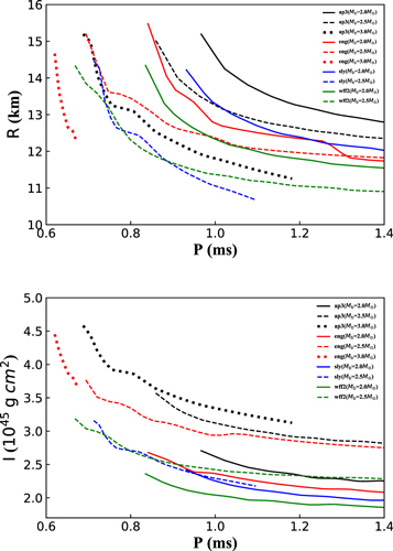
Figure 1. Evolutionary behavior of the NS radius (R) and moment of inertia (I) for different EoSs and baryonic mass.
Download figure:
Standard image High-resolution imageFor a given EoS, when the NS rotational speed is approaching the breakup limit, R and I approach to constant. As the NS spins down, both R and I would go through a rapid descent phase. When the spin is slow enough, R and I again tend to be constant. For a given rotational speed, the greater baryonic mass of the NS leads to a smaller R and greater I. For our selected EoSs, when the baryonic mass or rotational speed of an NS undergoes changes, the radius of the NS can vary from 10–15 km, and the moment of inertia of the NS can vary from 1.5 × 1045 to 4.5 × 1045 g cm2.
3. Numerical Results
With the solutions of R and I for various rotational speeds, for an NS with given parameters (e.g., given the initial values of Bp
, , Mb
, and P0), we can numerically solve its spin-down evolutionary history, and calculate the evolutionary history of magnetic dipole radiation luminosity. The result is obviously dependent on the NS EoS and different baryonic mass. For each of our selected EoSs and baryonic mass, we calculate the spin-down solutions for a large sample of NSs with various parameter combinations, where the NS spin-down process is dominated either by EM radiation or GW radiation. Here, we assume that the magnetic dipole moment μ ≡ Bp
R3 is conserved.
First, for EM radiation-dominated case, we set the initial values Bp,0 = 1015 G, P0 = 1 ms, and = 10−7. We test two values for Mb
(e.g., 2.0 and 2.5 M⊙), with which the NS can be supported by most of the adopted EoSs. In Figure 2(a), we plot the results for selected models that are relevant for reflecting the main conclusions, which can be summarized as follows:
4
- 1.For the situations when realistic values are considered or the fiducial values are assigned to R and I (e.g., R = 106 cm and I = 1.5 × 1045 g cm2), the magnetic dipole radiation luminosity could be different up to one order of magnitude. In this case, if one use the fiducial values to estimate the dipolar magnetic field strength and the initial spin period for the nascent NS, the results could be systemically biased.
- 2.For a given EoS, different NS baryonic mass could evidently alter the magnitude and evolutionary history of the dipole radiation luminosity. According to the results in Figure 2(a), with higher baryonic mass, the luminosity becomes smaller, and the spin-down timescale becomes larger. When the baryonic mass is large enough, the magnetar collapses into a black hole after slightly spinning down, so that the dipole radiation can suddenly enter a rapid descent phase.
- 3.For a given baryonic mass, different EoSs could change the overall magnitude of the dipole radiation luminosity. As shown in Figure 2(a), with a more stiff EoS, the luminosity generally becomes larger, and the spin-down timescale becomes smaller. Adopting different EoSs could change whether and when the magnetar would collapse.
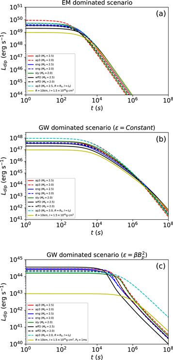
Figure 2. Numerical results for dipole radiation luminosity by considering the R and I evolutionary effects in the choice of different NS EoSs and baryonic mass of an NS. (a) EM-dominated scenario. We set Bp,0 = 1015 G and P0 = 1 ms for the initial condition, and = 10−7; (b) GW-dominated scenario with a constant ellipticity. We set Bp,0 = 1014 G and P0 = 1 ms for the initial condition, and = 10−3; (c) GW-dominated scenario with  . We set the initial condition as Bp,0 = 1012 G, 0 = 10−4. Here, we use the Kepler period for each adopted Mb
and EoS as the initial spinning period P0.
. We set the initial condition as Bp,0 = 1012 G, 0 = 10−4. Here, we use the Kepler period for each adopted Mb
and EoS as the initial spinning period P0.
Download figure:
Standard image High-resolution imageThen we consider the GW radiation-dominated case, where the intensity of GW radiation depends on the NS asymmetries (manifested by the value of ). Here, we discuss two mechanisms to induce NS asymmetries: first, the crust of an NS is solid and elastic, whereas the solid shape is related to the history of the NS formation and EoS (Haskell et al. 2006; Lasky 2015), in which scheme the value is usually assumed to be a constant during the spin-down process (Corsi & Mészáros 2009; Lasky & Glampedakis 2016; Lü et al. 2017, 2019; Sarin et al. 2018; Lan et al. 2020; Sur & Haskell 2021). Second, the NS asymmetry is caused by the distortion of the NS magnetic field, in which scheme the ellipticity satisfies  (Bonazzola & Gourgoulhon 1996; Haskell et al. 2008; Dall'Osso et al. 2009, 2018; Gao et al. 2017a; Lander & Jones 2020). Similarly, two values of Mb
(e.g., 2.0 and 2.5 M⊙) are tested. In Figures 2(b) and (c), we plot the results for both scenarios, which can be summarized as follows:
(Bonazzola & Gourgoulhon 1996; Haskell et al. 2008; Dall'Osso et al. 2009, 2018; Gao et al. 2017a; Lander & Jones 2020). Similarly, two values of Mb
(e.g., 2.0 and 2.5 M⊙) are tested. In Figures 2(b) and (c), we plot the results for both scenarios, which can be summarized as follows:
- 1.For both scenarios, with realistic values of R and I for different EoSs and NS baryonic mass being considered, the magnetic dipole radiation luminosity could be variant up to one order of magnitude. Similar to the EM radiation-dominated case, if one use the fiducial values of R and I to estimate properties of the nascent NS, the results would be significantly biased.
- 2.The history of magnetic dipole radiation luminosity for both scenarios would consist of four segments. The first two segments are Ldip ∝ t0 followed by Ldip ∝ t−γ . The last two segments would be Ldip ∝ t−1 followed by Ldip ∝ t−2. The emergence of a new segment Ldip ∝ t−γ is due to the evolution of R and I. When is approximated to be a constant, γ is slightly smaller than 1; when
 , γ is around or larger than 3.

In previous works, it has been proposed to obtain the braking index of the nascent NS by fitting the magnetic dipole radiation luminosity with
where n is the braking index with  ,
,  is defined as the NS spin-down luminosity and
  is defined as the spin-down timescale of the NS. The obtained braking index is then used to diagnose whether the magnetar spin-down is dominated by EM radiation or GW radiation (Lasky et al. 2017; Lü et al. 2019), since when EM radiation dominates, the torque equation becomes
  , so that the braking index becomes 3. On the other hand, when GW emission dominates, the torque equation becomes
  , so that the braking index becomes 5. According to our results, when the newly born NS has a millisecond spin period, R and I are no longer constant, so that if one still applies Equation (6) to fit the magnetic dipole radiation luminosity, the obtained braking index could be slightly smaller than 3 for the EM emission-dominated case or greatly smaller than 3 for the GW emission-dominated case with constant
  , or larger than 5 for the GW emission-dominated case with constant . l
On the other hand, our results show that the sharp decay t−(>3) following the X-ray plateaus (Rowlinson et al. 2010, 2013; Lü et al. 2015; Sarin et al. 2020a) is unnecessarily related to the collapse of the central magnetar. Instead, it could be caused by the R and I evolutionary effect, if the spin-down process of the nascent NS is dominated by GW radiation and the ellipticity satisfies  . If our interpretation is correct, this may explain why some GRBs that present the internal plateau feature, still show late-time central engine activity, manifested through flares and second shallow plateaus (Troja et al. 2007; Perley et al. 2009; Margutti et al. 2011; Gao et al. 2015, 2017b; Zhao et al. 2020). In the magnetar collapse scenario, only flares or plateaus close to the internal plateau can be interpreted with the fallback accretion model (Chen et al. 2017; Zhao et al. 2020).
4. Analytical Analysis of the Numerical Results
Under certain approximations, we can try to explain the results from numerical calculation by an analytical method. By fitting the evolutionary behavior of R and I for different EoSs and baryonic mass, one can approximately get that
where R0, I0, and Ωk are the initial radius, initial moment of inertia, and Keplerian angular velocity of the newly born NS, respectively. It is worth noting that Ωk depends on the NS EoS and baryonic mass. m and k are the power-law indexes for R and I evolution with respect to the rotational speed of the NS. The best-fitting values of m and k for different EoSs and Mb are listed in Table 1. For our selected EoSs, m ranges from 0.21–0.38 and k ranges from 0.12–0.31. When the baryonic mass is large enough, the magnetar collapses into a black hole after slightly spinning down, in which case the values of m and k are denoted as "NO." With the assumption that the magnetic dipole moment μ ≡ Bp R3 is conserved, the evolution of Ldip can be derived based on Equation (2).
Table 1. The Evolution Indexes of R and I with different EoSs and NS Baryonic Mass
| m | ||||
|---|---|---|---|---|
| AP3 | ENG | SLy | WFF2 | |
| Mb = 2.0 M⊙ | 0.34 | 0.35 | 0.21 | 0.33 |
| Mb = 2.5 M⊙ | 0.27 | 0.28 | 0.37 | 0.27 |
| Mb = 3.0 M⊙ | 0.38 | NO | NO | NO |
| k | ||||
| AP3 | ENG | SLy | WFF2 | |
| Mb = 2.0 M⊙ | 0.14 | 0.13 | 0.13 | 0.12 |
| Mb = 2.5 M⊙ | 0.15 | 0.24 | 0.25 | 0.22 |
| Mb = 3.0 M⊙ | 0.31 | NO | NO | NO |
Download table as: ASCIITypeset image
(I) For the Ldip-dominated case, one has
so that the complete solution of Ω(t) in Equation (9) can be written as
where Ω0 is the initial angular frequency at t = 0, and Tsd,em is a corresponding characteristic spin-down timescale, which can be derived as
Hence, the evolutionary history of Ldip can be expressed as
where Lsd,em is the initial luminosity of the electromagnetic dipole emission at t = 0, which can be calculated as
It is clear that both the magnitude and the evolutionary history of Ldip depend on the realistic EoS and NS mass, as well as the evolutionary history of the moment of inertia (with index k). Comparing Equation (6) with Equation (12), one can obtain the braking index in this scenario as

When k > 0, we have n < 3.
(II) For LGW dominated case with keeping constant, one has
so that the complete solution of Ω(t) in Equation (15) could be written as
where Tsd,gw could be derived as
The evolution history of Ldip could be expressed as
Similar to the EM-dominated case, here both the magnitude and the evolution history of Ldip depend on the realistic EoSs and NS mass, as well as the evolution history of the moment of inertia (with index k). Comparing Equation (6) with Equation (18), one can derive the braking index in this scenario as

When k > 0, we have n > 5.
(III) For the LGW-dominated case with  , one has
so that the complete solution of Ω(t) in Equation (20) can be written as
where Tsd,gw can be derived as
The evolutionary history of Ldip can be expressed as
In this case, the evolutionary history of Ldip not only depends on the evolutionary history of the moment of inertia I, but also the evolutionary history of R. The decaying power-law index 4/(12m − k − 4) could be around or larger than 3. Comparing Equation (6) with Equation (23), one can derive the braking index in this scenario as

which could be much smaller than 5 (even smaller than 3).
5. Conclusion and Discussion
By solving the field equations, we find that when a NS's rotational speed is approaching the breakup limit, its radius and moment of inertia undergoes an obvious evolution as the NS spins down. In this case, the deceleration history of the NS becomes more complicated for a given initial dipole magnetic field and ellipticity. Our main results can be summarized as follows:
- 1.When realistic values of R and I for different EoSs and NS baryonic mass are considered, the magnetic dipole radiation luminosity can be variant within one to two orders of magnitude.
- 2.With the consideration of R and I evolutionary effects for a rapidly spinning NS, its magnetic dipole radiation light curve presents new segments. For instance, when GW radiation dominates the spin-down power and, the history of magnetic dipole radiation luminosity then consists of four segments, i.e., Ldip ∝ t0 followed by Ldip ∝ t−γ
, and then followed by Ldip ∝ t−1 and Ldip ∝ t−2. The new segment Ldip ∝ t−γ
with γ larger than 3 is due to the evolution of R and I. In this case, if one applies to fit the dipole radiation luminosity, the obtained braking index could be much smaller than 3.
5
- 3.In the case when the EM radiation power is comparable to the GW radiation power, the dipole radiation light curve becomes even more complicated. Especially when the initial EM radiation power is slightly larger, for scenario, there will be a transition from EM loss dominating to GW loss dominating, and then back again as the NS spins down. In this case, the history of dipole radiation consists of five segments, i.e., Ldip ∝ t0 followed by Ldip ∝ t−2 and then followed by Ldip ∝ t−γ
(γ is larger than 3), and then followed by Ldip ∝ t−1, and finally followed by Ldip ∝ t−2. For those complicated situations, Equation (6) may not be a good formula to fit the dipole light curve. But if one still applies Equation (6) to find the braking index, the result could vary from n < 3 to n > 5, depending on how many segments being covered by the observations.


According to our results, (1) we suggest that when using the EM observations such as the X-ray plateau data of GRBs to diagnose the properties of the nascent NSs, NS EoS and mass information should be invoked as simultaneously constrained parameters; (2) if the spin-down process of the nascent NS is dominated by GW radiation and the ellipticity satisfies  , the sharp decay following the X-ray plateau could be caused by the R and I evolutionary effect rather than due to the NS collapsing. If this is true, it may explain why some GRBs that present the internal plateau feature still show late-time central engine activity, manifested through flares and second shallow plateaus. Future EM and GW joint detection could help to distinguish these two scenarios.
Finally, we would like to point out several caveats regarding our results. First, the physical conditions for a nascent NS would be very complicated, and some conditions may significantly alter the radiation light curve, so that the R/I evolutionary effect we discussed here would be reduced or even completely suppressed. For instance, it has been proposed that the evolution of the inclination angle between the rotation and magnetic axes of the NS could markedly revise the X-ray emission (Çıkıntoğlu et al. 2020). Moreover, the nascent NS is likely to undergo free precession in the early stages of its lifetime when the rotation and magnetic axes of the system are not orthogonal to each other, which would lead to the fluctuations in the X-ray light curve (Suvorov & Kokkotas 2020, 2021). On the other hand, the X-ray plateau emission luminosity could emerge from a plerion-like model of the nascent NS, in which model the magnetized, relativistic wind from a millisecond magnetar injects shock-accelerated electrons into a cavity confined by the GRB blast wave. The plerion model introduces an anticorrelation between the luminosity and duration of the plateau, and also shows a sudden drop in the X-ray emission when the central magnetar collapses into a black hole (Strang & Melatos 2019).
Second, even if the NS EoS and mass information were invoked as we suggest, one may still face many difficulties when using the X-ray plateau data of GRBs to diagnose the properties of the nascent NS. For instance, precise estimation for the luminosity of X-ray plateaus, in many cases, is very difficult to obtain because there are no redshift measurements for most GRBs and the uncertainties introduced by the cosmological k-correction could also be significant (Bloom et al. 2001). On the other hand, a constant efficiency is usually assumed to convert the spin-down luminosity to the observed X-ray luminosity, which might be incorrect. It has been proposed that the efficiency might be strongly dependent on the energy injecting luminosity, which leads to a larger braking index from afterglow fitting compared to the case with constant efficiency (Xiao & Dai 2019). Furthermore, if one considers both energy injection and radiative energy loss of the blast wave, the X-ray light curve would be altered without changing the braking index, and this model could also fit the data well (Dall'Osso et al. 2011; Sarin et al. 2020b).
Finally, it is worth noting that besides the magnetar scenario, many alternative models have been proposed to interpret the X-ray plateau emission, such as the structure jet model (Beniamini et al. 2020), the high-latitude emission model (Oganesyan et al. 2020), the late-time energy injection model (Matsumoto et al. 2020), etc. As suggested by Sarin et al. (2019), before attempting to derive NS parameters, one should first ensure that the magnetar scenario is the preferred hypothesis.
We thank the anonymous referee for the helpful comments that have helped us to improve the presentation of the paper. L.L., H.G., and S.Z.L. acknowledge the support of the National Natural Science Foundation of China under grant Nos. 11722324, 11690024, and 11633001, the Strategic Priority Research Program of the Chinese Academy of Sciences under grant No. XDB23040100, and the Fundamental Research Funds for the Central Universities.
Footnotes
- 3
- 4
Here, we did not show any cases in which the NS collapses during the spin-down process.
- 5
Other reasons why the braking index could be smaller than 3 has been discussed in Lasky et al. (2017).