


Abstract
We have examined the Ne/O and Fe/O characteristics of large solar energetic particle (SEP) events at the ion energy range of 3–40 MeV nucleon−1 during solar cycles 23 and 24. In each cycle, the solar activity displays an ∼3 yr rising phase and a longer declining phase. While Fe-poor events only appeared in the declining phase of cycle 23, the properties of Fe-rich events were similar in the rising phases of both cycles. Also, very few Fe-rich events were seen in the declining phase of cycle 24. In addition, the Ne/O data in the corona, solar wind, and SEP events consistently reveal that the characteristics of SEP events are mainly governed by the solar wind turbulence status that exhibits a significant difference between slow and fast streams. During the rising phase of the solar cycles, slow streams are dominated by the two-dimensional turbulence component, which significantly reduces the injection energy of the quasi-perpendicular (Q-Perp) shock acceleration. Also, slow streams have an increased Ne/O ratio and hence enhanced temperature of coronal suprathermals, favoring the occurrence of Fe-rich events. In contrast, in the declining phase of the solar cycles, the fast streams are dominated by the slab turbulence component, which could significantly increase the injection energy of the Q-Perp shock acceleration. Consequently, in fast streams, most Fe-rich events originate from jet suprathermals. The coronal suprathermals may produce the Fe-poor events having abnormally low Ne/O ratios provided the speed of the associated coronal mass ejection is large enough.
Export citation and abstract BibTeX RIS
1. Introduction
1.1. Current Status of Ion Ratio Studies in Large SEP Events
In Tan et al. (2017), we began the analysis of the highly variable spectral and compositional characteristics of large solar energetic particle (SEP) events at higher energies by introducing the model of Tylka & Lee (2006), which provides a reasonable description of the high-energy asymptotic behavior of ion ratios in gradual SEP events (Reames 2013). In addition, the critical assumptions of the model are confirmed by simulations (e.g., Sandroos & Vainio 2007; Yang et al. 2011). Here we consider the further use of the model in the examination of long-term variations of large SEP events during solar cycles 23 and 24.
According to the model, at high ion energies (>20 MeV nucleon−1), SEP events are roughly divided into two groups. The "Fe-poor" event with the Fe/O ratio falling with energy is a bigger event having a softer spectrum and exponential rollover. In contrast, the "Fe-rich" event with the Fe/O ratio increasing with energy is a smaller event showing a harder spectrum that is nearly a power law and has no rollover (Tylka et al. 2005; Zank et al. 2006). The high-energy variability of ion ratios is assumed to be caused by "the interplay of two factors: evolution in the shock-normal angle as the shock moves outward from the Sun; and a compound seed population, typically comprising at least suprathermals from the corona (or solar wind) and suprathermals from flares." (Tylka & Lee 2006). In view of the progress of SEP studies since the model was established, it is necessary to evaluate these factors to justify whether they are still consistent with new observational facts and theoretical models.
In this section, we consider the issue of seed populations of SEPs. The concept of suprathermals from flares comes from the evidence that the 3He-rich impulsive SEP events are associated with flares on the Sun. However, further observations exhibit that the flares associated with impulsive SEP events are often observed in the forms of more-energetic jets from solar active regions (ARs; Bučík et al. 2018a, 2018b), indicating that the magnetic reconnection involving open field lines allows SEPs and narrow coronal mass ejections (CMEs) to escape (Kahler et al. 2001). The probable temperature of the source plasma in the impulsive SEP event is cooler (2.5–3.2 MK; see Reames et al. 2014a, 2014b, and 2015) than the typical temperatures (10–40 MK) of the flares that are involved in reconnection on closed field lines where SEPs are trapped. Therefore, instead of the suprathermals from flares, we prefer to call them suprathermals originating from jets (e.g., Bučík 2020).
Also, the difference between the coronal and solar wind suprathermals has been emphasized. The solar corona supports two kinds of solar wind flows, the fast solar wind (FSW) that escapes along the open field lines of coronal holes (CHs) and the slow solar wind (SSW) that arises at the boundaries of CHs or over closed field structures (Wang et al. 1996; Schwadron et al. 1999; Posner et al. 2001). The main difference in seed populations between SEPs and the SSW appears in the fractionation process, which reveals the variation of elemental abundances as a function of the first ionization potential (FIP). Low-FIP elements, ionized in the chromosphere, are more efficiently conveyed upward to the corona than high-FIP elements that are initially neutral atoms (Webber 1975; Meyer 1985).
While the FIP bias, i.e., the ratio of the elemental abundance levels at low and high FIPs, is smaller in the FSW, the bias is similar between SEPs and the SSW (Bochsler 2009). Nevertheless, the FIP difference between SEPs and the SSW is mainly exhibited in the intermediate elements with FIP ∼ 10–14 eV, especially C, P, and S. For example, relative to the photospheric abundance, if the SEP abundance and the 1.2 times SSW abundance are plotted as a function of FIP, a crossover from low to high is seen at FIP ∼ 10 eV in SEPs but FIP ∼ 14 eV in the SSW (Reames 2018a, 2018b; Laming et al. 2019). The difference is consistent with the previous results (Mewaldt et al. 2002; Desai et al. 2003) that SEPs cannot be merely the accelerated bulk solar wind or its suprathermal tail.
Also, it is noted that no significant compositional or energy spectral differences of SEP events exist between the SSW and FSW (Kahler & Reames 2003; Kahler et al. 2009), indicating that the seed population of SEPs should be an independent sample of coronal material (Reames 2018a, 2018b).
Theoretically, the difference between SEPs and the SSW can be explained in terms of Alfvénic turbulence interacting with the density gradient that generates the ponderomotive force, which is a time-averaged nonlinear force acting on media in the presence of oscillating electromagnetic fields (Laming 2015, 2017; Laming et al. 2019). The force compels the charged particle to move toward the area of weaker field strength. When particles expand from the chromosphere up into the corona, the force can act on ions but not neutral atoms. Consequently, low-FIP elements, ionized in the chromosphere, are more efficiently conveyed upward to the corona than high-FIP elements that are initially neutral atoms. Therefore, the source plasma that will eventually be shock-accelerated to be SEPs should originate in magnetic structures where the Alfvénic turbulence resonates with the loop length on closed magnetic field lines with a high fractionation (Laming 2015; Reames 2018a, 2018b; Laming et al. 2019). In contrast, the source of the SSW may be located near the base of the surrounding open field lines but outside of ARs, where such resonance does not exist.
In fact, Alfvén waves with a coronal origin, where they may be created by nanoflares, are at or close to resonance with the coronal loop, offering a significantly better match to observed abundances than photospheric waves (Laming 2017). Therefore, in the upper corona, where the CME-driven shock begins (∼1.5 times the solar radius), the turbulence environment should be different from the lower corona, where the fractionation happens. This new viewpoint would emphasize that SEPs are not merely the accelerated solar wind. Nevertheless, observations reveal that in the high- or low-FIP region, the elemental abundance of SEPs is close to that of the SSW. This point is important to explain why Ne/O variations in coronal, SSW, and SEP events are comparable (see detailed discussion in Section 4.2) because of the high-FIP feature of the Ne element.
1.2. Incident Energy Threshold of CME-driven Shock Acceleration
We then consider the θBn dependence of the incident energy threshold in the CME-driven shock acceleration process, where θBn is the angle between the shock normal and the upstream magnetic field direction. The dependence is understandable because highly oblique shocks have a high injection threshold (at least, coronal suprathermals cannot be accelerated in the context of diffusion theory; Zank et al. 2006).
In fact, in the diffusive shock acceleration theory, the occurrence of ion acceleration depends on the presence of perpendicular diffusion of accelerated particles (Schwadron et al. 2015). A superposition of slab and two-dimensional (2D) turbulence components is necessary in order to develop a transverse complexity in the magnetic field, which leads the perpendicular transport of particles to be diffusive (Matthaeus et al. 1995, 2003; Zank et al. 2004). In addition, the solar wind turbulence observation is consistent with a composite model of slab and 2D turbulence components (Matthaeus et al. 1990; Tu & Marsch 1993; Bieber et al. 1994) that describe the solar wind turbulence statuses parallel and perpendicular to the magnetic field, respectively. The injection energy threshold of CME-driven shock-accelerated ions is strongly dependent on the fraction of the 2D turbulence component relative to the slab turbulence component in the solar wind (Zank et al. 2006).
Since the CME height at the metric type II radio burst onset is ∼1.5 Rs, where Rs is the solar radius (Gopalswamy et al. 2012), the rapid expansion of the CME should result in a quasi-perpendicular (Q-Perp) shock structure close the Sun (<2 Rs) and a quasi-parallel (Q-Par) shock structure farther out (>2.5 Rs) (Schwadron et al. 2015). Thus, SEPs are produced in the height range of ∼1.5–10 Rs, which is also confirmed by the onset time analysis of SEP events (Reames 2009a, 2009b; Tan et al. 2013). Therefore, SEPs should be produced in the higher corona, where the turbulence status is different from the lower corona. In fact, in the lower corona, the source plasma that is eventually shock-accelerated to SEPs should originate in magnetic structures where Alfvénic turbulence resonates with the loop length on closed magnetic field lines (Laming 2015; Reames 2018a, 2018b; Laming et al. 2019).
In the solar wind, the earlier analysis carried out at 1 au (Bieber et al. 1996; Leamon et al. 1998) pointed out that the magnitude fraction of the slab turbulence power in the inertial range is only ∼20%. In a later analysis, when the constraint by the fitting function format is added, Hamilton et al. (2008) reported that the magnitude fractions of Alfvén turbulence in the inertial range are ∼20% and ∼50% in the SSW and FSW, respectively. In addition, although the turbulence fraction has not been measured in the range of 1.5–10 Rs, where the CME-driven shock acceleration occurs, recent Parker Solar Probe (PSP) observations (e.g., Adhikari et al. 2020a; Zhao et al. 2020) have shown that near the Sun, the statistical analysis result is consistent with the turbulence in the SSW consisting of a majority 2D component and a minority slab component (Zank et al. 2017), but in the FSW (Adhikari et al. 2020b), the Alfvénic turbulence is dominant (Goldreich & Sridhar 1995; Montgomery & Matthaeus 1995).
Zank et al. (2006) noted that in the solar wind, both the injection energy and the acceleration timescale at highly perpendicular shocks are sensitive to the assumption of the ratio of the 2D correlation length scale to the slab correlation length scale. The injection energy threshold will be decreased with the increase of the relative fraction of the 2D turbulence component. Equivalently, in the CME-driven shock, the injection energy threshold of accelerated particles would be decreased with the increase of the ratio of the perpendicular to the parallel diffusion coefficient (Schwadron et al. 2015), as described in Section 4.3.
Therefore, after evaluating the main factors that affect the high-energy variability of SEPs, the updated version of the Tylka & Lee model assumes the existence of two main groups of large SEP events: Fe-rich events resulting from jet suprathermals accelerated by Q-Perp shocks and Fe-poor events resulting from coronal suprathermals accelerated by Q-Par shocks. Is there any new group of large SEP events? We try to answer this question by examining the observation of long-term variations of Ne/O and Fe/O ratios. However, in order to realize this goal, we need to expand our previous work (Tan et al. 2017, hereafter T17), as described below.
1.3. Our Previous Work on Ne/O and Fe/O Studies during Solar Cycle 23
While the importance of Ne/O studies was mentioned in earlier works (e.g., Reames et al. 1994; Mewaldt et al. 2007), a systematic analysis of Ne/O and Fe/O data began from T17. The first motivation of the analysis came from the observations (e.g., Tylka et al. 2005) that the ion energy (Ei) dependence of Fe/O ratios includes the interplanetary (IP) transport effect. Since the IP transport is an ion rigidity–dependent process (Reames 2013), the effect depends on the mass-to-charge ratio A/Q of the ions.
Reames et al. (1994) noted that in the impulsive SEP event, C, N, and O, like He, are probably fully ionized with A/Q ∼ 2.0, while Ne, Mg, and Si form a group that might correspond to a two-electron closed shell with A/Q ∼ 2.3, and Fe has A/Q ∼ 3.6. These ionization levels correspond to the source plasma temperature of T = 2.5–3.2 MK (Reames 2017) that appears in coronal ARs. In addition, in the gradual SEP events examined by Reames (2016), 69% of events show T = 0.8–1.6 MK, which is consistent with the acceleration of ambient coronal thermals by CME-driven shocks. In contrast, 24% of gradual SEP events show T = 2.5–3.2 MK, typical of that in the coronal ARs previously determined from the impulsive SEP event.
Because the A/Q value of Fe and O ions is significantly different, through the IP transport process, Fe ions could stay ahead of O ions, resulting in the increase and decrease of Fe/O values during the earlier and later phases of an SEP event, respectively (Tylka et al. 2013). In contrast, since the A/Q value is similar between Ne and O ions, the time variation of Ne/O values would be small. Consequently, a combination analysis of Ne/O and Fe/O data could diminish the IP transport effect.
However, as shown in Figure 3 of T17, the high-energy variation ranges of the Ne/O and Fe/O ratios derived from the model of Tylka & Lee (2006) are 1–3 and 0.3–6, respectively. Note that these values are normalized to their nominal coronal values (0.152 and 0.134 for Ne/O and Fe/O, respectively) in Table 9.1 of Reames (1999). In view of a smaller variation range of Ne/O, we need to improve the accuracy of the Ne/O measurements. However, in the available data sets of heavy ions in the range Ei = 3–40 MeV nucleon−1, various ion species have different measured intervals of Ei, leading to the ion intensity estimated at different nominal Ei values. We ought to first derive the intensities of Ne and O ions at the same nominal Ei value before going to calculate the Ne/O ratio. Therefore, in T17, we developed a technique to estimate the ion ratio at the same Ei value by rebinning the ion intensity data in the form of equal bin widths in the logarithmic energy scale.
In recent works, the observed results of Ne/O and Fe/O are often expressed as Ne/O/0.157 and Fe/O/0.131, respectively, where 0.157 and 0.131 are the averaged elemental abundances of Ne and Fe relative to O as determined from all SEP events examined by Reames (2014). These values are then defined as the new nominal values of SEP events in Table 1 of Reames (2018b).
During solar cycle 23 for the large SEP events with Jpp(>60 MeV) >1 pfu (the particle flux unit = 1 cm−2 s−1 sr−1), where Jpp is the peak proton intensity measured by the GOES Energetic Particle Sensor (EPS), the Ne/O data sampled in the decay phase of SEP events can be divided into two groups: (1) Ne/O/0.157(24 MeV nucleon−1) > 1, which corresponds to Fe/O/0.131(24 MeV nucleon−1) > 1, i.e., the Fe-rich event caused by suprathermals from jets; and (2) Ne/O/0.157(24 MeV nucleon−1) ≤ 1, with some events even having Ne/O/0.157 < 0.7, which implies the absence of jet suprathermals. It is seen that in the events of group 2, the observed Fe/O/0.131 value at low energies (Ei < 10 MeV nucleon−1) could be greater than 1. The enhanced Fe/O ratio is assumed to be due to the IP transport effect, which could be diminished by normalizing the Fe/O ratio to that measured at Ei = 6 MeV nucleon−1. The ratio of Fe/O(Ei) to Fe/O(6 MeV nucleon−1) is then used to classify SEP events at high energies. However, Fe-rich features are still seen in the events of group 2.
The situation is similar when the source plasma temperature T is compared between the two groups of SEP events. By using the T data independently determined by Reames (2016), it is seen that the presence of correlations between T and Ne/O implies that Ne/O is a rough proxy of T. However, while the high- and low-Ne/O events correspond to the Fe-rich and Fe-poor groups, respectively, in the middle Ne/O range, the correlation between Fe/O and Ne/O (T) is very poor. In particular, there exist Fe-rich events with lower Ne/O values, indicating the importance of further analysis of SEP events with Ne/O/0.157(24 MeV nucleon−1) ≤ 1.
1.4. Issues to Be Addressed in This Work
Except for the necessity of further analysis of low-Ne/O events, as explained above, other issues also exist in T17 that are addressed in a comprehensive way in the current work.
- (1)Because the low-energy increase of Fe/O and Ne/O due to the streaming limited proton intensity (Reames & Ng 2010) is significant in large SEP events, in the Wind Low Energy Matrix Telescope (LEMT) Ei range (3–12 MeV nucleon−1), the best examination of ion ratios should be carried out at Ei = 6–12 MeV nucleon−1. However, even in such an Ei range, it is seen from T17 that a number of large SEP events have Ne/O/0.157 ∼ 0.7. Are these low-Ne/O events due to the statistical fluctuation of Ne/O distributions or belonging to a new group with different event features?
- (2)Recent observations from the SUMER streamer measurements (Landi & Testa 2015) and the ACE/SWICS solar wind measurements (Shearer et al. 2014) consistently pointed out that the Ne/O value in the solar wind significantly varies during a solar cycle. The Ne/O value is nearly constant in the fast wind and correlates strongly with the solar activity in the slow wind. Especially, in the slow wind, Ne/O is inversely correlated with the solar wind speed (Vsw; Shearer et al. 2014). How does the variation of Ne/O ratios in a solar cycle affect the SEP event accelerated by CME-driven shocks?
- (3)In the model of Tylka & Lee (2006), the difference between Q-Perp and Q-Par accelerated events is the difference of the θBn ranges over which the model spectrum is averaged (integrated): θBn = 0°–90° for the Q-Perp shock and θBn = 0°–60° for the Q-Par shock. In a given θBn range, the energy of the seed particles should exceed the injection energy threshold of shock acceleration, which depends on the solar wind turbulence status. As explained in Section 1.2, the turbulence status is different between slow and fast streams. Therefore, we need to examine the ion ratio measurements in various solar activity phases in order to understand the effect of θBn.
- (4)In T17, we only examined the Ne/O and Fe/O data during solar cycle 23. Since the solar activity during solar cycle 24 was significantly diminished (Gopalswamy et al. 2020), the comparison of ion ratio observations between solar cycles 23 and 24 is important in order to understand how the solar activity variation affects the occurrence of large SEP events. In particular, the simulation of Giacalone (2015) showed that a weak interplanetary magnetic field (IMF) could reduce the intensity of SEP events because a weak field would decrease the diffusion coefficient of SEPs, allowing charged particles with lower energies to escape from the shock front. Although the simulation is made for the proton intensity peak caused by the IP shock at 1 au, its basic idea that a low magnitude of the IMF can lead to the intensity decrease of shock-accelerated particles can be tested by using various SEP populations (e.g., Raukunen et al. 2016; Reames 2018b; Kahler & Ling 2019). Also, the simulation of Vainio et al. (2017) showed that the lack of large SEP events in cycle 24 is due to the reduction of coronal plasma and suprathermal densities. We will verify whether, in large SEP events, the ion ratio observations support these simulations.
We first present the observed data and analysis technique in Section 2. We then report the main observations in Section 3 and discuss their implications in Section 4. Finally, we summarize the main findings in Section 5.
2. Observed Data and Analysis Technique
2.1. Data Sources
We use the proton intensity data measured by the EPS on the GOES spacecraft to display the time profile of proton intensities at the proton energy Ep > 60 MeV. Also, the GOES/High Energy Proton and Alpha Detector (HEPAD) provides the high-energy proton intensity data in the range Ep = 375–605 MeV.
The low-energy ion data in the range Ei = 3–12 MeV nucleon−1 are obtained from the LEMT of the Energetic Particle Acceleration, Composition, and Transport (EPACT) experiment on the Wind spacecraft (von Rosenvinge et al. 1995). Since LEMT is a large-geometry (51 cm2 sr) instrument, its onboard processing system can resolve elements from He through about Pb at a rate of up to about 104 particles s–1.
The high-energy ion intensity data in the range Ei = 8.5–40 MeV nucleon−1 are obtained from the Solar Isotope Spectrometer (SIS) on the ACE spacecraft (Stone et al. 1998). The SIS also provides good accuracy of measurements because of its large-geometry factor (32 cm2 sr).
In addition, IMF and solar wind data, as well as solar and magnetic indices, are obtained from the Space Physics Data Facility (SPDF) OMNIWeb Data Explorer.
2.2. Analysis Technique
2.2.1. Interpolation of Ion Intensity Data
As described in T17, in order to improve the accuracy of Ne/O measurements, the differential intensity (Ji) data of both Ne and O ions are given at the same nominal Ei value. Since the Ei bins in the original Wind/LEMT and ACE/SIS data sets show different locations and widths for various ion species, we need to adjust them before calculating the Ne/O ratio.
In view of the fact that the ion spectrum is usually close to a power-law function, we rebin the Ji data into the form of equal bin widths in the logarithmic energy scale (for details, see T17). At each time instant, the measured value of ln(Ji) versus ln(Ei) is approximated by a polynomial function. An iteration procedure is then used to derive the fitting parameter from which the fitted value Ji and its standard deviation (σJi) are obtained at a given interval i, whose lower limit El(i) is

and the upper limit is Eu(i) = El(i + 1). The nominal value of Ei(i) = (El(i)Eu(i))1/2, whose unit is MeV nucleon−1.
Since at Ei = 9.5 MeV nucleon−1, we have two fitted values of Ne/O (also Fe/O) that are separately derived from the Wind/LEMT and ACE/SIS data sets, the consistency between the two values should be strong evidence to justify calibration and fitting procedures. Therefore, in Figure 1 at Ei = 9.5 MeV nucleon−1, the Ne/O/0.157 (Fe/O/0.131) value derived from the ACE/SIS data is plotted versus that from the Wind/LEMT data for the SEP events selected in the upper (lower) panel. The event selection criterion will be described in the next subsection. Note that in Figure 1, the observed result is expressed as Ne/O/0.157 and Fe/O/0.131, where 0.157 and 0.131 are the new nominal values of Ne/O and Fe/O in Table 1 of Reames (2018b), respectively. Also, the dashed line is the fitting result between the two data sets, which is very close to the diagonal line that indicates an exact equality between two values.
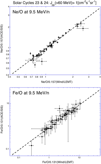
Figure 1. At Ei = 9.5 MeV nucleon−1, the Ne/O/0.157 (Fe/O/0.131) value derived from the ACE/SIS sensor is plotted vs. that from the Wind/LEMT sensor for SEP events selected in the upper (lower) panel. The dashed line is the least-squares fitting result between the two data sets.
Download figure:
Standard image High-resolution image2.2.2. Selection of Large SEP Events
We use the time profile of the proton intensity Jp data measured by the GOES/EPS at Ep > 60 MeV to select the so-called "large" SEP events. Background proton intensity has been subtracted from the observed Jp (>60 MeV) value. The large SEP event is defined as its peak value (Jpp) greater than 1 pfu, in spite of the necessary adequate adjustment (see T17).
For a typical event selected, the time profiles of the available particle data are plotted in Figure 2, which shows the last ground-level enhancement (GLE) of cycle 24 that occurred on 2017 September 10. The time profile of the background-subtracted Jpp(>60 MeV) is given in the first panel, where t0.1A, tpeak, and t0.1B are the times of Jp = 0.1Jpp in the rising phase, Jp = Jpp, and Jp = 0.1Jpp in the decay phase, respectively. The total duration of an event is defined as τt = t0.1B–t0.1A.
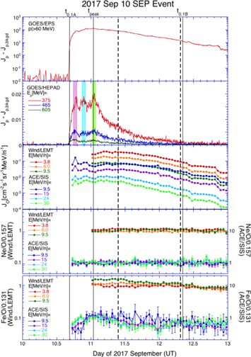
Figure 2. Time profiles of GOES/EPS >60 MeV proton intensities (first panel), GOES/HEPAD high-energy proton intensities (second panel), O ion intensities measured by both Wind/LEMT and ACE/SIS sensors (third panel), Ne/O/0.157 (i.e., the Ne/O ratio normalized to its nominal coronal value; fourth panel), and Fe/O/0.131 (i.e., the Fe/O ratio normalized to its nominal coronal value; fifth panel). Two dashed lines limit the sample period of the ion ratio calculation in the 2017 September 10 event.
Download figure:
Standard image High-resolution imageThe second panel displays the time profile of GOES/HEPAD background-subtracted high-energy proton intensity data that are given in a linear scale plot of proton intensities. It is seen that three peaks of proton intensities exhibit between t0.1A and tpeak, as denoted by the color strips, which provide the information on the high-energy proton injection.
Furthermore, the third panel shows the time profiles of O ion intensities (Jo) measured by both the Wind/LEMT and ACE/SIS sensors. Note that the green and blue dots denote the Ei = 9.5 MeV nucleon−1 data measured by LEMT and SIS, respectively. The coincidence between the corresponding green and blue dots is consistent with the calibration result given in Figure 1. Moreover, by comparing the first and third panels in Figure 2, we see that the decay phase of O ion intensities is later than that of Jp(>60 MeV). Consequently, the sample interval of ion ratio calculations previously defined as the length of the decay phase of Jp(>60 MeV) needs some adjustment (see T17). The final sample interval is limited between tstart and tstop, which are denoted by the two dashed lines in Figure 2.
Time profiles of Ne/O/0.157 and Fe/O/0.131 are shown in the fourth and fifth panels, respectively, from which it is seen that in the Ei range of 3–30 MeV nucleon−1, there is a constant value of Ne/O/0.157 ∼ 1, while the Fe/O/0.131 value displays an Ei dependence in the earlier stage of the decay phase.
As listed in Table 1, 29 and 18 events are selected during cycles 23 and 24, respectively. The 29 events of cycle 23 match those examined in T17. Later, these events are divided into Fe-richA, Fe-richB, and Fe-poor groups in Section 4.1. The classification of three events is uncertain because of a lack or poor quality of their Ne/O data.
Table 1. Characteristic Parameters of SEP Events with Jpp(>60 MeV) > 1 pfu during Solar Cycles 23 and 24
| Event | Classification | Flare Position | τr (hr) | Jpp (>60 MeV) (pfu) | tstart (days) | tstop (days) | Ne/O/0.157(24 MeV nucleon−1) | Fe/O/0.131(24 MeV nucleon−1) | T (MK) |
|---|---|---|---|---|---|---|---|---|---|
| 1997 Nov 4 | Fe-richB | S14W33 | 18 | 6 | 4.39 | 5.05 | 1.09 ± 0.07 | 3.21 ± 0.64 | 3.2 ± 0.3 |
| 1997 Nov 6 | Fe-richA | S18W63 | 26 | 90 | 6.77 | 7.65 | 1.74 ± 0.03 | 6.04 ± 0.57 | 2.5 ± 0.2 |
| 1998 Apr 20 | Fe-poor | S22W90 | 39 | 44 | 21.57 | 22.60 | 0.67 ± 0.01 | 0.06 ± 0.02 | ≤0.8+0.2 |
| 1998 May 2 | Fe-richA | S15W15 | 19 | 17 | 2.63 | 3.38 | 1.75 ± 0.10 | 5.34 ± 0.80 | 2.5 ± 0.1 |
| 1998 May 6 | Fe-richA | S11W65 | 11 | 11 | 6.38 | 6.80 | 1.67 ± 0.13 | 3.77 ± 1.41 | 2.7 ± 0.3 |
| 1998 Aug 24 | Fe-richB | N35E09 | 33 | 8 | 25.08 | 25.50 | 0.87 ± 0.11 | 1.33 ± 0.34 | 1.6 ± 0.2 |
| 1998 Sep 30 | Fe-richB | N23W81 | 13 | 13 | 30.81 | 31.15 | 1.13 ± 0.04 | 1.64 ± 0.40 | 1.3 ± 0.2 |
| 1998 Nov 14 | Fe-richA | N28W90 | 11 | 16 | 14.80 | 15.30 | 1.55 ± 0.06 | 4.11 ± 0.64 | 2.9 ± 0.4 |
| 2000 Jul 14 | Fe-poor | N22W07 | 30 | 1050 | 14.70 | 15.20 | 1.05 ± 0.03 | 0.49 ± 0.23 | 1.16 ± 0.2 |
| 2000 Nov 8 | Fe-poor | N10W77 | 22 | 1180 | 9.15 | 9.50 | 0.72 ± 0.03 | 0.14 ± 0.04 | 1.16 ± 0.2 |
| 2001 Apr 2 | Fe-richA | N19W72 | 25 | 26 | 3.32 | 4.11 | 1.78 ± 0.04 | 1.92 ± 0.49 | 3.0 ± 0.3 |
| 2001 Apr 15 | Fe-richB | S20W85 | 11 | 239 | 15.80 | 16.10 | 1.09 ± 0.06 | 4.41 ± 0.37 | 3.1 ± 0.4 |
| 2001 Apr 18 | Fe-richB | >SW90 | 21 | 26 | 18.25 | 19.01 | 0.99 ± 0.06 | 1.65 ± 0.50 | 3.0 ± 1.0 |
| 2001 Aug 15 | Fe-poor | >SW90 | 9 | 91 | 16.30 | 16.60 | 0.87 ± 0.03 | 0.69 ± 0.13 | 1.4 ± 0.4 |
| 2001 Sep 24 | Fe-poor | S16E23 | 46 | 127 | 25.32 | 25.75 | 0.66 ± 0.02 | 0.27 ± 0.04 | 0.9 ± 0.3 |
| 2001 Nov 4 | Fe-poor | N06W18 | 44 | 185 | 5.15 | 5.60 | 0.77 ± 0.02 | 0.18 ± 0.09 | 0.9 ± 0.3 |
| 2001 Dec 26 | Fe-richB | N08W54 | 8 | 124 | 26.31 | 26.65 | 0.83 ± 0.03 | 3.66 ± 1.88 | 1.6 ± 0.2 |
| 2002 Apr 21 | Fe-poor | S14W84 | 42 | 105 | 21.45 | 22.85 | 0.87 ± 0.02 | 0.13 ± 0.04 | ≤0.8+0.2 |
| 2002 Aug 22 | Fe-richA | S07W62 | 20 | 4 | 22.23 | 22.96 | 2.00 ± 0.24 | 4.87 ± 1.39 | 3.2 ± 0.5 |
| 2002 Aug 24 | Fe-richB | S02W81 | 11 | 59 | 24.30 | 24.80 | 0.92 ± 0.07 | 2.45 ± 0.97 | |
| 2003 Oct 26 | Fe-richB | N02W38 | 14 | 4 | 26.82 | 27.50 | 0.81 ± 0.03 | 1.21 ± 0.33 | 1.6 ± 0.3 |
| 2003 Oct 28 | Fe-poor | S16E08 | 17 | 851 | 28.60 | 28.90 | 0.63 ± 0.02 | 0.18 ± 0.08 | ≤0.8+0.2 |
| 2003 Oct 29 | Fe-richA | S15W02 | 23 | 254 | 30.00 | 30.40 | 1.36 ± 0.04 | 0.97 ± 0.11 | 2.5 ± 0.4 |
| 2003 Nov 2 | Fe-poor | S14W56 | 13 | 99 | 2.82 | 3.40 | 0.86 ± 0.03 | 0.38 ± 0.22 | 1.0 ± 0.3 |
| 2005 Jan 15 | Fe-poor | N15W05 | 31 | 5 | 16.63 | 17.35 | 1.19 ± 0.04 | 0.29 ± 0.09 | 1.0 ± 0.4 |
| 2005 Jan 17 | Fe-poor | N15W25 | 27 | 157 | 17.70 | 18.70 | 1.16 ± 0.02 | 0.16 ± 0.07 | 0.8 ± 1.0 |
| 2005 Jan 20 | Fe-richA | N14W61 | 10 | 906 | 20.33 | 20.71 | 1.53 ± 0.04 | 1.65 ± 0.70 | 2.0 ± 1.0 |
| 2005 Jun 16 | N08W90 | 18 | 7 | 17.00 | 17.65 | 1.78 ± 0.55 | 3.24 ± 0.75 | ||
| 2006 Dec 13 | Fe-richA | S06W23 | 14 | 185 | 13.40 | 13.80 | 1.30 ± 0.03 | 5.08 ± 0.52 | 2.0 ± 0.2 |
| 2011 Jun 7 | Fe-richB | S21W54 | 27 | 8 | 7.55 | 8.40 | 1.06 ± 0.19 | 2.69 ± 0.77 | |
| 2011 Aug 4 | Fe-richB | N19W36 | 17 | 4 | 4.40 | 4.90 | 1.01 ± 0.10 | 2.61 ± 0.46 | 3.2 ± 0.5 |
| 2011 Aug 9 | Fe-richA | N17W69 | 8 | 5 | 9.37 | 9.70 | 2.61 ± 0.32 | 5.39 ± 1.14 | |
| 2012 Jan 23 | Fe-richB | N28W21 | 32 | 15 | 23.40 | 24.30 | 0.75 ± 0.04 | 1.6 ± 0.2 | |
| 2012 Jan 27 | Fe-richB | N27W71 | 30 | 23 | 28.20 | 29.00 | 0.81 ± 0.03 | 0.43 ± 0.12 | |
| 2012 Mar 7 | Fe-richB | N17E27 | 50 | 160 | 7.60 | 8.40 | 1.23 ± 0.02 | 0.81 ± 0.24 | |
| 2012 Mar 13 | Fe-richB | N17W66 | 10 | 11 | 13.80 | 14.13 | 0.75 ± 0.11 | 2.78 ± 0.55 | |
| 2012 May 17 | Fe-richB | N11W76 | 10 | 36 | 17.24 | 17.50 | 0.81 ± 0.11 | 1.96 ± 0.27 | |
| 2012 Jul 19 | Fe-richB | S13W88 | 18 | 2 | 19.50 | 20.05 | 1.17 ± 0.14 | 3.17 ± 1.26 | |
| 2012 Jul 23 | Fe-richB | >W90 | 67 | 2 | 23.80 | 25.00 | 0.85 ± 0.08 | 0.68 ± 0.11 | |
| 2013 Apr 11 | Fe-richB | N09E12 | 25 | 5 | 11.55 | 12.40 | 1.18 ± 0.29 | 4.44 ± 1.99 | 2.0 ± 0.3 |
| 2013 May 22 | Fe-richB | N15W70 | 32 | 11 | 23.10 | 23.90 | 0.81 ± 0.06 | 1.17 ± 0.33 | 1.0 ± 0.4 |
| 2014 Jan 6 | >W90 | 24 | 5 | 6.60 | 7.30 | 7.80 ± 2.17 | 2.9 ± 0.4 | ||
| 2014 Jan 7 | Fe-richB | S15W11 | 28 | 16 | 8.20 | 9.00 | 0.78 ± 0.03 | 0.58 ± 0.16 | 1.2 ± 0.5 |
| 2014 Feb 25 | Fe-richB | S12E82 | 86 | 2 | 25.90 | 27.00 | 1.17 ± 0.11 | 7.22 ± 1.61 | |
| 2014 Apr 18 | Fe-richB | S20W34 | 18 | 2 | 18.80 | 19.30 | 1.09 ± 0.15 | 2.12 ± 1.07 | 2.8 ± 0.3 |
| 2014 Sep 11 | N14E02 | 38 | 2 | 11.25 | 11.70 | 4.07 ± 0.83 | |||
| 2017 Sep 10 | Fe-richB | >W90 | 40 | 130 | 11.40 | 12.30 | 1.11 ± 0.02 | 0.56 ± 0.12 |
Note. (1) Fe-richA and Fe-richB are the high-energy Fe-rich events caused by jet and coronal suprathermals, respectively. Here Fe-poor is the high-energy Fe-poor event caused by coronal suprathermals. (2) Here τt is the total width of an event. (3) 1 pfu = 1 cm−2 sr−1 s−1. (4) Here tstart and tstop are the start and stop times (days) of the sampled period in the ion ratio calculation. (5) The T data are taken from Table 5 of Reames (2016) with the addition by D. Reames.
Download table as: ASCIITypeset image
2.2.3. Elemental Abundance in SEP Events
In order to understand the distribution details of elemental abundances, we need to estimate the standard deviation σ of the distribution. We start the estimation of σ from Figure 10 of Reames (2014), which is adapted as Figure 3 in this work, where the filled dots denote the elemental abundance averaged over the SEP events as a function of Ei. Also, the overall energy average of the elemental abundances is denoted by the black solid bar.
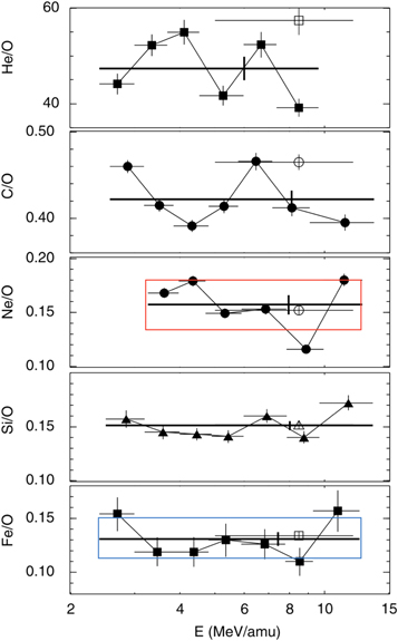
Figure 3. Element abundances, averaged over all SEP events examined by Reames (2014), are shown as a function of Ei as filled symbols, and the overall energy averages are shown as solid bars. Open symbols show the corresponding abundances from Reames (1995). The figure is adapted from Figure 10 of Reames (2014) with the red (blue) box added to denote the width of the Ne/O (Fe/O) distribution (i.e., twice the standard deviation σ).
Download figure:
Standard image High-resolution imageBased on the measurements from Figure 3, we derive the nominal elemental abundance ratios Ne/O/0.157 = 1 ± σNe/O and Fe/O/0.131 = 1 ± σFe/O, where σNe/O = 0.15 and σFe/O = 0.14 are consistent with the final estimation of Reames (2016). Thus, in Figure 3, the widths of the red and blue boxes along the ordinate are equal to 2σNe/O and 2σFe/O, respectively.
It is seen that in large SEP events, the ion ratio measurement is disturbed by a large background at low energies. As shown in Figure 7.9 of Reames (2021) for the 2000 July 4 (the "Bastille-Day") SEP event, the background stretches all the way up to the 2–20 MeV range. Fortunately, the background corresponds to the Ei (energy per nucleon) range of heavy ions at ≤1 MeV nucleon−1. On the other hand, due to the effect of the streaming limited proton intensity (Reames & Ng 2010), the enhancement of Fe/O and Ne/O in the large SEP events is seen below Ei ∼ 6 MeV nucleon−1 (see T17). Therefore, the reasonable examination range of ion ratios should be reduced to Ei = 6–12 MeV nucleon−1. However, even within the reduced Ei range, there is no guarantee that the nominal elemental abundance ratio of Reames (2018b) as derived from all SEP events examined by Reames (2014) could be applied to the large SEP events selected in this work. Consequently, we will reserve the nominal Ne/O or Fe/O value of Reames (2018b) as a reference and observe its difference from the measured value.
3. Observations
3.1. Ion Energy Dependence of Ne/O Ratios
Profiles of Ei dependence for the Ne/O/0.157 values derived from the selected SEP events in Table 1 are plotted in the left and right columns of Figure 4 for solar cycles 23 and 24, respectively. Two events (the 2005 June 16 and 2014 September 11 events) are not included in Figure 4 because of missing or poor-quality Ne/O data. In addition, in Figure 4, the pink strip is the red box of Figure 3 but with its energy window reduced to 6–12 MeV nucleon−1. Depending on the position relative to the pink strip, the observed data in each solar cycle are divided into three groups having Ne/O/0.157 > 1+σNe/O (upper panels), 1 − σNe/O < Ne/O/0.157 < 1+σNe/O (middle panels), and Ne/O/0.157 < 1 − σNe/O (lower panels).
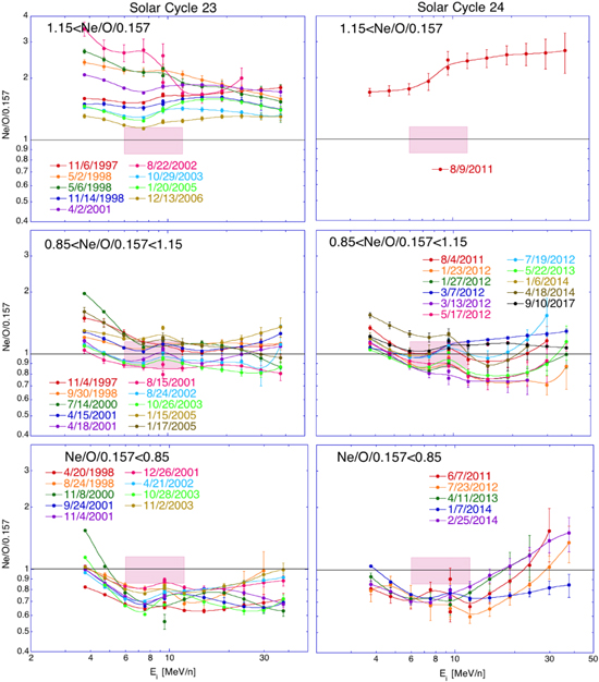
Figure 4. The time profiles of the Ei dependence of Ne/O/0.157 are plotted in the left and right columns for solar cycles 23 and 24, respectively, where the pink strip is the red box of Figure 3 with its Ei range reduced to 6–12 MeV nucleon−1. In addition, in each cycle (column), we divide the observed data into three panels with Ne/O/0.157 > 1+σNe/O (upper panels), 1 − σNe/O < Ne/O/0.157 < 1+σNe/O (middle panels), and Ne/O/0.157 < 1 − σNe/O (lower panels), where σNe/O = 0.15. Here two events (the 2005 June 16 and 2014 September 11 events) in Table 1 are not shown because of missing or poor-quality Ne/O data.
Download figure:
Standard image High-resolution imageFirst, we see the difference of the observed Ne/O ratios between the two columns (solar cycles): (1) as shown in the upper panels, there are nine events with Ne/O/0.157 > 1+σNe/O in cycle 23, while in cycle 24, there is only one event in such an Ne/O range; and (2) when Ne/O/0.157 < 1+σNe/O (middle and lower panels) at Ei > 6 MeV nucleon−1, the Ei dependence of Ne/O is weak in cycle 23 but strong in cycle 24. In particular, in cycle 24, the Ne/O ratio in the lower panel significantly increases with energies at Ei > 20 MeV nucleon−1.
Second, in the same cycle, we see the difference of the observed Ne/O energy distributions among different panels. The prominent feature of the distributions found is the presence of a large number of events with lower Ne/O ratios (lower panels). For example, in cycle 23, we have nine events below the pink strip, in contrast to 10 events inside the pink strip. According to a Gaussian distribution, the ratio of the event number below the pink strip (between 1σNe/O and 2σNe/O) to that inside the pink strip (between −1σNe/O and 1σNe/O) should be 0.2, which is significantly less than the observed value (0.9), indicating that the low-Ne/O group has an origin different from that of the group inside the pink strip.
3.2. Comparison of Fe/O Observations with the Tylka & Lee Model
As explained in T17, the use of Ne/O data can diminish the IP transport effect. Therefore, similar to the Ne/O data shown in Figure 4, the Ei dependence of the Fe/O/0.131 values is shown in Figure 5, where the light blue strip denotes the blue box in Figure 3 with its energy window reduced to Ei = 6–12 MeV nucleon−1. Note that in Figure 5, the division of the different panels is based on the Ne/O/0.157 ranges shown in Figure 4.

Figure 5. The time profiles of the Ei dependence of Fe/O/0.131 are plotted in the left and right columns for solar cycles 23 and 24, respectively, where the light blue strip is the blue box of Figure 3 with its Ei range reduced to 6–12 MeV nucleon−1. In addition, in each cycle (column), we divide the observed data into three panels according to the ranges of Ne/O/0.157 shown in Figure 4.
Download figure:
Standard image High-resolution imageFrom Figure 5, the following features of the Fe/O/0.131 distributions are seen: (1) the events with Ne/O/0.157 > 1+σNe (upper panels) correspond to Fe/O/0.131 > 1+σFe, which is consistent with jet suprathermals producing the Fe-rich events (see Section 1.1); (2) in the absence of jet suprathermals (middle and lower panels), the Fe/O/0.131 value at low energies may be significantly greater than 1, which should be due to the IP transport effect (Reames 2014, 2016); and (3) when Ne/O/0.157 < 1 − σNe/O (lower panels), at Ei > 12 MeV nucleon−1 in cycle 23, most SEP events have Fe/O/0.131 < 0.5, whereas in cycle 24, none of the events exhibit Fe/O/0.131 < 0.5.
In order to distinguish between Fe-rich and Fe-poor events at high energies, we need to perform a more quantitative comparison of our observations with the model of Tylka & Lee (2006). We hence display the event-integrated Fe/O/0.134 (0.134 is the old nominal Fe/O ratio of SEPs in Reames 1999) value predicted by the model as a function of the ion kinetic energy (Ei0) in Figure 6, which is adapted from Figure 5(a) in Tylka & Lee (2006), showing calculations in which the injection of ions from the coronal component is suppressed at Q-Perp shocks. The suppression is realized by adding a heuristic weighting factor (~cos(θBn)) to the integrated expression of ion intensity for the coronal component, so that the coronal contribution is suppressed as the shock approaches perpendicular. Otherwise, as Tylka & Lee (2006) showed in their Figure 5(b), there is no increase in Fe/O at high energies. However, observations (e.g., Figure 10 in Tylka et al. 2005 and Figure 5 in this work) reveal that in most of the Fe-rich events, the Fe/O ratio is increased with Ei increasing at Ei > 12 MeV nucleon−1. Also, further simulations (e.g., Sandroos & Vainio 2007; Yang et al. 2011) indicate that such suppression is necessary.
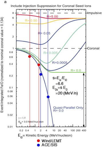
Figure 6. The event-integrated Fe/O/0.134 value predicted by the model of Tylka & Lee (2006) is plotted as a function of the ion kinetic energy (Ei0) for different values of a variable factor R that quantifies the relative magnitude of the jet and coronal components in the seed population as defined by Equation (2). The figure is adapted from Figure 5(a) in Tylka & Lee (2006), showing calculations in which the injection of ions from the coronal component is suppressed at Q-Perp shocks. Since the e-folding energy E0 is the only energy scale in the model, the curve in the figure can be shifted horizontally by changing the scale factor s = Eis/Ei0, where Eis is the observed ion kinetic energy. In addition, the observed minimum of the Fe/O/0.134 values in each panel of Figure 7 is plotted as a filled dot having its abscissa equal to Ei0 = Eis/s with s = 6.6 (see text).
Download figure:
Standard image High-resolution imageFurthermore, note that Figure 6 is presented under the following model parameters.
- (1)The low-energy power-law spectral index γ = 1.5, which corresponds to the shock compression ratio r = 2.5 for nonrelativistic particles produced in the diffusive shock acceleration process (Ellison & Ramaty 1985). Interestingly, a study of the spectral properties of 46 isolated, large SEP events carried out by Desai et al. (2016a, 2016b, 2016c; ∼10 yr later than the work of Tylka & Lee) showed that γ has "an event-averaged mean of ∼1.64 ± 0.03, with 1σ standard deviation of ∼0.6", see Desai et al. (2016b). In addition, for 33 near-Sun CME shocks, the average compression ratio inferred from their spectral index is r = 2.49 ± 0.08 (Desai et al. 2016b), indicating the reasonability of the γ = 1.5 assumption.
- (2)The e-folding energy E0 = 3 MeV nucleon−1, which reflects the restriction of the acceleration process imposed by the limited size of the acceleration regions (Schwadron et al. 2015). This assumed E0 value is located at the maximum of the transition energy distribution of SEPs as shown in Figure 6 of Desai et al. (2016b). In addition, from Table 1 of Desai et al. (2016c), it is seen that among the 46 examined events, there are 27 events having finite 3He/4He ratios, whose values range from (6.1 ± 2.5) × 10−4 to (7.8 ± 0.5) × 10−2 with a mean value of 9.2 × 10⁻³. In view of the averaged 3He/4He values of (4.08 ± 0.25) × 10−4 and (3.3 ± 0.3) × 10−4 in the SSW and FSW, respectively (see Gloeckler & Geiss 1998), these events should belong to the 3He-rich event group. Also, from Table 1 of Desai et al. (2016c), it is seen that these 3He-rich events have an average intersection energy of 3.1 ± 2.8 MeV nucleon−1. Therefore, the E0 = 3 MeV nucleon−1 assumption is appropriate for the acceleration of jet suprathermals by Q-Perp shocks.
In the model of Tylka & Lee (2006), the parameter Ci is a normalization coefficient, proportional to the relative abundance of ion species i in the seed population. The relative magnitude of the jet and coronal components in the seed population is defined by using O ions in the variable

which is a free parameter in the model. Note that R reflects the relative strengths of the two components as they are viewed in a parallel shock, where the issue of suppressed injection does not arise. In Figure 6, R > 0 corresponds to Fe/O/0.134 > 1. However, when R = 0 (lack of jet suprathermals) at high energies (Ei0 > E0), we have Fe/O/0.134 ∼ 0.3 for the Q-Perp shock acceleration and Fe/O/0.134 < 0.1 for the Q-Par shock acceleration.
Generally speaking, for any SEP event, its e-folding energy can be expressed as E0s = s E0, where s is a scale factor. Fortunately, since E0s is the only energy variable in the model, the curve in Figure 6 can be shifted horizontally by changing the scale factor s = Eis/Ei0, where Eis and Ei0 are the observed ion energy and the ion energy denoted by the abscissa of Figure 6, respectively. Below, we derive the s value for the acceleration of coronal suprathermals by Q-Par shocks based on the scaling principle.
In Figure 6, the lower blue line that represents the Q-Par shock acceleration at R = 0 gives the minimum of Fe/O/0.134 values measured at a given Ei0. In order to derive the s value of the lower blue line, we show the Fe/O/0.134 data found during cycle 23 in Figure 7, where the Fe/O/0.134 value as measured at different energies Eis is plotted versus the total duration τt of the SEP events. In each panel of the figure, the two dashed lines denote the maximum and minimum values of the measured Fe/O/0.134 data at a given Eis. Since, in Figure 7, none of the observed events has an Fe/O value that always equals the minimum of the Fe/O/0.134 values ((Fe/O)i,min) in each Eis channel, we construct a virtual event whose ordinate value is equal to (Fe/O)i,min in all Eis channels. In Figure 6, along the lower blue line, the abscissa value of the (Fe/O)i,min point determines the Ei0 value given at E0 = 3 MeV nucleon−1, from which the scale factor si = Eis/Ei0 can be derived. Then, a mean value of s (∼6.6) is calculated from the derived si values. Note that this mean s value is close to the upper boundary (s = 6) of the transition energy distribution of SEPs shown in Figure 6 of Desai et al. (2016b). Also, by using this mean s value, the observed (Fe/O)i,min data points are plotted in Figure 6 as filled dots. Since the scaled E0s = s E0 ∼ 20 MeV nucleon−1, in the acceleration of coronal suprathermals by Q-Par shocks, the Fe/O/0.134 value should be dropped to <0.3 at Eis > 20 MeV nucleon−1.
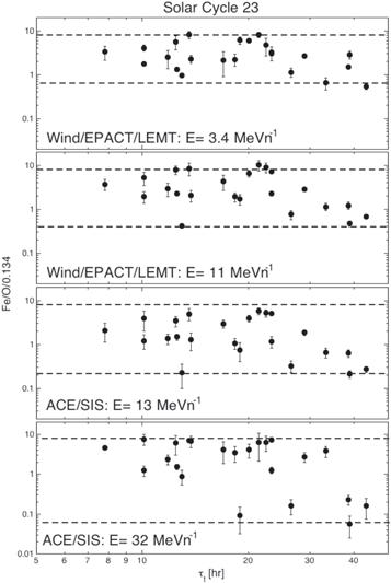
Figure 7. The Fe/O/0.134 data are plotted vs. the total width tt of the SEP events as measured at different energy Eis values during cycle 23. In each panel, two dashed lines denote the upper and lower boundaries of the measured Fe/O/0.134 values.
Download figure:
Standard image High-resolution imageFor the Ne/O/0.157 ≤ 1 event, the apparent Fe/O/0.131 > 1 at low energies could be due to the IP transport effect, which can be diminished by normalizing the Fe/O/0.131 value to that at Ei = 6 MeV nucleon−1. Thus, we replot the middle and lower panels of Figure 5 in Figure 8, using Fe/O(Ei)/Fe/O(6 MeV nucleon−1) as the ordinate. In addition, in Figure 8, the light green strip denotes the region of Fe/O(Ei)/Fe/O(6 MeV nucleon−1) = 0.3 ± 0.1, which is the lower boundary of Fe-rich events at high energies (>20 MeV nucleon−1) according to Figure 6. Thus, in Figure 8, if the continuous decrease of Fe/O at high energies causes the Fe/O curve to drop below the light green strip, the event should be an Fe-poor event produced by Q-Par shock acceleration. In contrast, if the Fe/O curve is above the light green strip or significantly increased after passing a minimum, the event should be an Fe-rich event produced by Q-Perp shock acceleration. As listed in Table 1, among all observed events in the two cycles, there are 11 Fe-poor events, which all occurred in cycle 23.
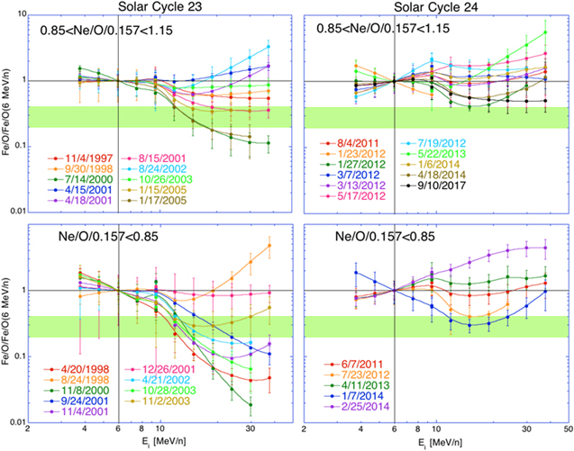
Figure 8. Using Fe/O(Ei)/Fe/O(6 MeV nucleon−1) as the ordinate, the middle and lower panels of Figure 5 are replotted here. In the figure, the light green strip denotes the region of Fe/O(Ei)/Fe/O(6 MeV nucleon−1) = 0.3 ± 0.1, which is the lower boundary of Fe-rich events at high energies (>20 MeV nucleon−1) according to Figure 6.
Download figure:
Standard image High-resolution image3.3. Solar Cycle Variations of Solar Activity Indices and SEP Characteristics
We show the time profiles of the solar activity parameters, including the daily sunspot number (first panel), IMF magnitude B (second panel), solar wind speed Vsw (third panel), and dynamical pressure of solar wind Pdyn (fourth panel), in solar cycles 23 and 24 in Figure 9, where the Jpp(>60 MeV) value of selected SEP events is given in the bottom panel.

Figure 9. Time profiles of solar activity parameters including the daily sunspot number (first panel), IMF magnitude B (second panel), solar wind speed Vsw (third panel), and dynamical pressure of solar wind Pdyn (fourth panel) during solar cycles 23 and 24. The two blue lines on the left (right) side limit the rising phase of cycle 23 (24), and the red line is the weighted average result of the solar activity parameters. In addition, the Jpp(>60 MeV) values of the SEP events selected are shown in the fifth panel, where the light blue bar is the median value of Jpp(>60 MeV) in the rising phase.
Download figure:
Standard image High-resolution imageCycle 23 can be further divided into an ∼3 yr rising phase (limited by the two left blue lines) and an ∼7 yr declining phase that is followed by an ∼4 yr minimum solar activity period. Also, cycle 24 can be divided into an ∼3 yr rising phase (limited by the two right blue lines) and an ∼6 yr declining phase. Because of the lack of strong ARs and CMEs (Lamy et al. 2019; Gopalswamy et al. 2020) and the record-low IMF intensity, reduced IMF turbulence activity, and solar wind dynamic pressure (Mewaldt et al. 2010), no large SEP event was found during the solar minimum between 2007 and 2011.
Here we first compare the rising phase with the declining phase in cycle 23. It is seen from Figure 9 that all solar wind parameters (B, Vsw, and Pdyn) in the rising phase were lower than those in the declining phase. In particular, slow streams (Vsw < 400 km s−1) were seen in the rising phase, while fast streams (Vsw > 500 km s−1) were seen in the declining phase. On the other hand, most of the SEP events found in the rising phase were Fe-rich (only one Fe-poor event was associated with a flare located at longitude 90°W), while both Fe-poor and Fe-rich events of larger magnitudes were evenly distributed in the declining phase of cycle 23.
The difference in solar activity parameters between the rising and declining phases is similar between cycles 23 and 24, although the absolute value of these parameters in cycle 24 is significantly lower than that in cycle 23. Therefore, it is surprising that the SEP properties, including the Fe-rich origin and average event intensity, are similar in both rising phases. This point can be clearly seen in the fifth panel of Figure 9, where the median values of Jpp(>60 MeV) for the SEP events selected, as denoted by the light blue bar, have nearly the same value in both rising phases.
Furthermore, we examine the variation of SEP characteristics in Figure 10, where the time profiles of the flare longitude of SEP events (second panel), speed VCME of CMEs (third panel), Jpp(>60 MeV) value (fourth panel), Jpp(>10 MeV) value (fifth panel), Ne/O/0.157(24 MeV nucleon−1) value (sixth panel), and Fe/O/0.131(24 MeV nucleon−1) value (seventh panel) are shown. In addition, the sunspot number is plotted in the first panel for reference.

Figure 10. Time profiles of the SEP event characteristics, including the solar longitude of SEP events (second panel), CME speed VCME (third panel), Jpp(>60 MeV) value (fourth panel), Jpp(>10 MeV) value (fifth panel), Ne/O/0.157 value measured at 24 MeV nucleon−1 (sixth panel), and Fe/O/0.131 value measured at 24 MeV nucleon−1 (seventh panel) are shown. In addition, the daily sunspot number is plotted in the first panel for reference.
Download figure:
Standard image High-resolution imageWe first compare SEP characteristics between the rising and declining phases of cycle 23. While the flare longitude of the SEP events in the two phases is similar, the VCME value in the declining phase is much higher than that in the rising phase, leading to a larger magnitude of Jpp(>10 MeV) and Jpp(>60 MeV) in the declining phase. In addition, Ne/O/0.157 = 1 + σNe/O is denoted by the horizontal dashed line in the Ne/O panel, from which it is seen that in the declining phase, both seed populations with Ne/O/0.157 > 1 + σNe/O and Ne/O/0.157 < 1 + σNe/O can produce the Fe-rich event, while only the seed populations with Ne/O/0.157 < 1 + σNe/O produce the Fe-poor event.
Furthermore, we compare the rising phases of both cycles 23 and 24. Note that in Figure 10, the light blue bars are also used to denote the median values of the SEP parameters. As mentioned above, the mean characteristics of the SEP events are similar in both rising phases, which can be seen from the similar location of the corresponding light blue bars. On the other hand, the solar wind parameters, including B, Vsw, and Pdyn, in cycle 24 are significantly lower than those in cycle 23.
Also, in the declining phase of cycle 24, the number of Fe-rich events is very small, which could be relevant to the low VCME values as shown in Figure 10.
Finally, we compare our observations with the theoretical works of Giacalone (2015) and Vainio et al. (2017). As mentioned above, through simulations, Giacalone (2015) suggested that the IMF magnitude (B) is an important factor affecting the SEP production. Moreover, from diffusive shock theory and simulation studies, Vainio et al. (2017) found that the lack of large SEP events, as well as the lack of high-A/Q ion species in cycle 24, are due to the reduction of coronal plasma and suprathermal densities.
However, our observations in Figures 9 and 10 show that during the two cycles, the mean characteristics of the SEP events are similar in both rising phases, which can be seen from the similar locations of the corresponding light blue bars. Since the solar wind parameters, including B, Vsw, and Pdyn, in cycle 24 are significantly lower than those in cycle 23, our results are inconsistent with the above theoretical works. Nevertheless, as explained in Section 4, our results are consistent with the observational examinations by Raukunen et al. (2016), Reames (2018b), and Kahler & Ling (2019).
4. Discussion
4.1. Characteristics of Particle Ratios at High Energies
Since the model of Tylka & Lee only predicts the high-energy asymptotic behavior of differential ion intensities, it is important to compare the measured ion ratios with the model prediction at high energies. Therefore, we first plot the Fe/O/0.131 data versus the Ne/O/0.157 data; both are measured at Ei = 24 MeV nucleon−1, in the upper panel of Figure 11, where the red and blue dots denote the Fe-poor and Fe-rich events, respectively. In addition, the vertical dashed line displays Ne/O/0.157 = 1 + σNe/O, and the horizontal red and blue lines show Fe/O/0.131 = 0.5 and 1, respectively. It is seen from the panel that except for a few points on the left side of the vertical line, all red or blue dots are located below the red line or above the blue line. The location difference indicates the Fe-poor origin of the red dots and the Fe-rich origin of the blue dots. Therefore, the event classification using the Fe/O ratio measured at Ei = 24 MeV nucleon−1 is similar to that using the Ei dependence of ion ratios as given by Figures 5 and 8, implying that the high-energy Fe/O ratio is less affected by the normalization procedure applied to Figure 8. This feature is important in the practical application because it provides a possibility of the SEP event classification only based on the ion ratio measured at a single higher-energy value of ions.

Figure 11. The Fe/O/0.131(24 MeV nucleon−1) value (upper panel), total width of SEP events (τt, middle panel), and plasma temperature (T, lower panel) of SEP events selected are plotted vs. Ne/O/0.157(24 MeV nucleon−1). In the figure, red and blue dots denote the Fe-poor and Fe-rich events, respectively. Also, the vertical line denotes Ne/O/0.131(24 MeV nucleon−1) = 1 + σNe/O, and the dashed line shows the least-squares fitting result.
Download figure:
Standard image High-resolution imageFurthermore, we add more characteristic parameters of SEP events, including the event total width (τt, middle panel) and plasma temperature (T, lower panel), in Figure 11, where the dashed line shows the least-squares fitting result. It is seen that the fitting result is generally good for the SEP events originating from jet superthermals with Ne/O/0.157 > 1 + σNe/O, as located on the right side of the vertical line.
Here we examine the T plot in the lower panel, where the horizontal red and blue lines show T = 1.2 and 2 MK, respectively. Reames (2014, 2015) developed a new method to determine the plasma temperature of seed populations in SEP events. Since particle transport in SEP events varies as a power-law function of A/Q, and Q varies with T, one can use the power-law form to find the T value that gives the best-fit pattern of the A/Q dependence of ion ratios.
On the right side of the vertical line, there are 11 Fe-rich events that have lower boundaries of Fe/O/0.131 = 1 (upper panel) and T = 2 MK (lower panel). In Table 1, these events are named the "Fe-richA" events that originate from the jet suprathermals having Ne/O/0.157(24 MeV nucleon−1) > 1 + σNe/O. Since the nature of the 2005 June 6 event is uncertain because of a large error bar of Ne/O data (although it should be Fe-rich in origin), the real number of Fe-richA events is 10, among which the 2011 August 9 event lacks T data. The Fe-richA event has T = 2.0–3.2 MK, which is a typical temperature over coronal ARs previously determined from the impulsive SEP events.
In contrast, on the left side of the vertical line, there are 11 Fe-poor events. As given in Table 1 of Reames (2016), the range of their T values is between 0.8 and 1.3 MK with a mean of 1.0 MK. Except for one event that is associated with a flare located at a longitude >90°W, these events have upper boundaries of T = 1.2 MK (lower panel) and Fe/O/0.131 = 0.5 (upper panel), indicating that they are the Fe-poor events originating from the low-temperature coronal suprathermals having Ne/O/0.157(24 MeV nucleon−1) < 1 + σNe/O. A positive correlation exists between Fe/O and Ne/O and between T and Ne/O for Fe-poor events, as shown in the upper and lower panels of Figure 11, respectively. In fact, from Figure 1 of Reames (2016), it is seen that Ne/O is increased with T increasing at T > 0.6 MK.
However, on the left side of the vertical line of Figure 11, there are Fe-rich events whose distributions exhibit large scattering. In Table 1, they are denoted as the "Fe-richB" events originating from the coronal suprathermals having Ne/O/0.157 ≤ 1 + σNe/O.
Among the 47 selected large SEP events, the fraction of Fe-richA events is 21%, which is consistent with 24% of the SEP events examined by Reames (2016) having the typical temperature (2.5–3.2 MK) of coronal ARs. In contrast, the fractions of Fe-richB and Fe-poor events of Table 1 are 49% and 23%, respectively.
An important implication of Table 1 is that among the 69% of SEP events examined by Reames (2016) with low T values (T = 0.8–1.6 MK), there is a large fraction of coronal Fe-rich events. One might suppose they are Fe-richA, but from Figure 10, they are Ne-poor and not originating from jet suprathermals. Therefore, our data reveal that about half of the SEP events selected are the Fe-richB events originating from coronal suprathermals, which is in conflict with the initial assumption of Tylka & Lee (2006) that there exist two main groups of large SEP events: Fe-rich events resulting from jet suprathermals accelerated by Q-Perp shocks and Fe-poor events resulting from coronal suprathermals accelerated by Q-Par shocks. There perhaps exists a new group (Fe-richB) of large SEP events that originate from coronal suprathermals accelerated by Q-Perp shocks. Since the difference between Q-Perp and Q-Par shock acceleration events appears in the averaged (integrated) θBn range of the model spectrum (θBn = 0°–90° and θBn = 0°–60° for the Q-Perp and Q-Par shock acceleration processes, respectively), we need to examine the solar wind conditions affecting the integration range of θBn.
4.2. Variation of Ne and O Abundances in the Solar Wind
As described above, since at the theoretical equilibrium temperature T > 0.6 MK, Ne/O increases with increasing T, we are able to track the variation of T by analyzing the Ne/O data. Also, as explained in Section 1.1, since observations reveal that in the high- or low-FIP region, the elemental abundance of SEPs is close to that of the SSW, the Ne/O measurements in coronal, SSW, and SEP events should be comparable because of the high-FIP feature of the Ne element.
In the first panel of Figure 12, we show time profiles of Ne/O ratios from solar wind abundance measurements, including the ACE/SWICS ion spectrometry data (see Shearer et al. 2014) that exhibit the Vsw dependence of Ne/O in solar cycle 23. The Ne/O ratio, which is not reduced to the nominal Ne/O value, significantly depends on the solar cycle; the Ne/O value is nearly constant in the fast wind but strongly anticorrelated with Vsw in the slow wind (Shearer et al. 2014). Also, the panel includes the SOHO/SUMER high-resolution coronal-streamer spectral data of Landi & Testa (2015) and the SOHO/Coronal Diagnostic Spectrometer (CDS) data of Young (2005). These data are in agreement with the ACE/SWICS measurements, indicating that the Ne/O abundance ratio measured in the inner corona is nearly the same as in the solar wind.
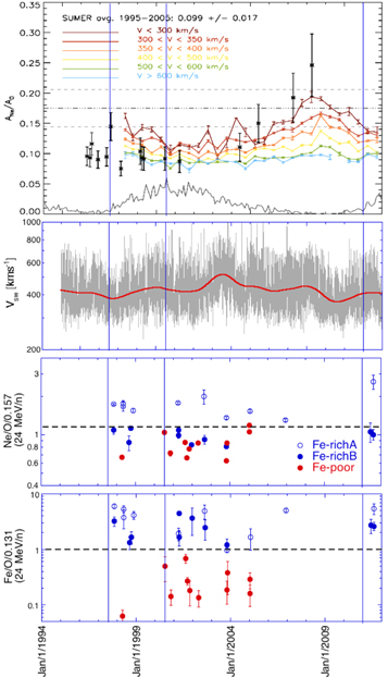
Figure 12. First panel: time profiles of Ne/O ratios from solar wind abundance measurements, including SOHO/SUMER (black dots), ACE/SWICS (colored dots), and SOHO/CDS (horizontal lines) data. Note that the Ne/O ratio is not reduced to the nominal Ne/O value. The monthly average sunspot number is shown as a solid gray line at the bottom. The panel is adapted from Figure 2 of Landi & Testa (2015). Other panels: time profiles of Vsw (second panel), Ne/O/0.157(24 MeV nucleon−1) (third panel), and Fe/O/0.131(24 MeV nucleon−1) (fourth panel). In the legend of the figure, Fe-richA and Fe-richB denote the high-energy Fe-rich events caused by jet and coronal suprathermals, respectively. In addition, Fe-poor denotes the high-energy Fe-poor event caused by coronal suprathermals. See the explanation of the vertical blue lines in Figure 9.
Download figure:
Standard image High-resolution imageThus, the comparison between coronal and in situ solar wind measurements of Ne/O ratios is consistent with a scenario that the solar wind can be divided into two broad classes: a slow wind with lower Vsw and coronal composition identical to that of coronal streamers, and a fast wind with higher Vsw, as originates from the centers of CHs because these regions are characterized by the least flux-tube expansion (Wang & Sheeley 1990). The difference in turbulence status between the two solar wind classes should originate from the upper corona (see Section 1.1).
As shown in the second panel of Figure 12, in the rising phase of cycle 23, slow streams have Vsw < 400 km s−1, while in the declining phase, fast streams can reach Vsw > 500 km s−1. Here we estimate the difference of plasma temperatures between the two phases. It is seen from the first panel that in the rising phase, the Ne/O value at Vsw < 400 km s−1 is ∼0.15, while at the declining phase, the Ne/O value at Vsw > 500 km s−1 is ∼0.09 (note a nearly constant Ne/O value in the fast wind). As a result, the nominal Ne/O values (i.e., Ne/O/0.157) thus derived are 1.0 and 0.6 in the rising and declining phases, respectively. Furthermore, from the bottom panel of Figure 11, it is seen that for Fe-poor events, the decrease of Ne/O/0.157 values from 1.0 to 0.6 corresponds to the decrease of T values from 1.2 to 0.8 MK. Therefore, compared with the declining phase, the rising phase should have an increment of △T ∼ 0.4 MK.
What is the effect of such a △T value? In the CME-driven shock acceleration process, coronal suprathermals display a κ-distribution (Vasyliunas 1968), where κ is a model parameter defining the strength of the suprathermal tail. Laming et al. (2013) discussed the shape variation of the κ distribution due to different choices of κ values. As an example, here we cite the κ distribution used by Battarbee et al. (2013), where the representative speed parameter is

where kB is the Boltzmann constant and mp is the proton mass. The particle distribution function is
where v is the particle speed, n is the particle number density, and Γ(x) denotes the gamma function. Battarbee et al. (2013) used κ = 2 for a distribution with a strong suprathermal tail and κ = 15 for a near-Maxwellian distribution. Since ω0 ∝ T1/2, for the suprathermal ions that have

we have

Thus,

Because T ∼ 1 MK and △T ∼ 0.4 MK, we have dlnT ∼ △T/T ∼ 0.4. Therefore, in the κ = 2 case of Battarbee et al. (2013), we have △f(v)/f(v) ∼ 0.6, indicating that the density of coronal suprathermals in the rising phase would have an ∼60% increment relative to that in the declining phase.
4.3. Difference between Slow and Fast Streams in the Solar Wind
In the rising phase of solar cycle 23, except for the increase of the number density of coronal suprathermals, as described above, the decrease of the injection energy threshold in the Q-Perp shock acceleration may affect the property of shock acceleration more significantly.
In fact, Dasso et al. (2005) observed that the feature of the solar wind anisotropy is significantly different between fast (>500 km s−1) and slow (<400 km s−1) streams. Fast streams are relatively more dominated by the slab turbulence component with the wavevector parallel to the local magnetic field B . In contrast, slow streams are more dominated by the 2D turbulence component with the wavevector perpendicular to B , which implies a more fully evolved turbulence status (see Section 1.2).
Because of the solenoidal nature of the magnetic field (Matthaeus et al. 1995), which implies that the Fourier component b ( k ) of the fluctuated magnetic field ( b ) at the wavenumber vector k should satisfy k · b ( k ) = 0, the magnetic fluctuation amplitude d b must be perpendicular to k . Therefore, in the SSW, the length of the parallel correlation scale (λ2D; i.e., the lobe aligned with the axis parallel to B in the Maltese cross of Matthaeus et al. 1990) is larger than that of the perpendicular correlation scale (λslab), and vice versa in the FSW.
In addition, Zank et al. (2006) examined the particle injection energy as a function of the shock obliquity in the diffusive shock acceleration process. For an IP shock located at 1 au, the injection energy threshold of particles is strongly dependent upon the θBn value as shown in their Figure 5, which is adapted as the upper panel of Figure 13 in this work. While the maximum injection threshold appears near θBn ∼ 90°, there is a singular point at θBn = 90°, where the threshold is decreased to be close to that at θBn = 0°. Also, the threshold value is strongly dependent upon the turbulence status. As the value of λ2D/λslab increases, the threshold value is decreased by more than 1 order of magnitude.

Figure 13. In the upper panel, for the seed particles injected into the diffusive shock acceleration mechanism in an IP shock located at 1 au, the injection energy is plotted as a function of the shock obliquity. Three possible ratios of λ2D and λslab are considered, where λ2D and λslab are the correlation scale lengths of the 2D and slab turbulence components, respectively. The figure is adapted from Figure 5 of Zank et al. (2006). In the lower panel, for the seed particles injected into the CME-driven shock acceleration mechanism, the injection energy is plotted as a function of the shock obliquity. Four possible ratios of the perpendicular-to-parallel diffusion coefficient are considered. The figure is adapted from Figure 3 of Schwadron et al. (2015).
Download figure:
Standard image High-resolution imageAs explained in Section 1.2, in the diffusive shock acceleration process, the increase of the relative fraction of the 2D turbulence component is equivalent to the increase of the relative magnitude of the perpendicular diffusion coefficient. Therefore, the θBn-dependence of the incident energy threshold in the CME-driven shock acceleration process as shown in Figure 3 in Schwadron et al. (2015) is adapted as the lower panel of Figure 13. The decrease of the injection energy with increasing the ratio of the perpendicular-to-parallel diffusion coefficient is apparent.
Here we qualitatively explain the change of injection energy threshold due to the variation of solar wind turbulence status by using the IP shock example of Zank et al. (2006). In the upper panel of Figure 13, we assume that the line of λ2D/λslab = 1 is representative of the turbulence status in slow streams during the rising phase, while the line of λ2D/λslab = 0.1 is representative of the fast streams during the declining phase. In addition, we use the blue and red arrows to denote the integrated ranges of θBn in the Q-Perp and Q-Par shock acceleration processes, respectively.
In the rising phase (solid line), the injection threshold Tinj is between 2 and 7 keV, which is reachable by both jet and coronal suprathemals, especially when the increase of the number density of coronal suprathermals due to the T increase has been taken into account. As shown in the third and fourth panels of Figure 12, in the rising phase, the jet suprathermal (open blue circles) and the coronal suprathermal (filled blue circles) can produce Fe-richA and Fe-richB events, respectively. That explains why, in the rising phase, most of the SEP events produced are Fe-rich in origin.
The situation is different in the declining phase, because from the λ2D/λslab = 0.1 line in Figure 13, we see that the maximum Tinj that occurs at θBn ∼ 80° is ∼40 keV. It is obvious that it is difficult for coronal suprathermals to reach such a high energy, and the Fe-richA event produced by jet suprathermals should be dominant. In contrast, in the θBn range that corresponds to the Q-Par shock acceleration, the value of Tinj is less than 10 keV, which is accessible by coronal suprathemals. That explains why the Fe-poor events appear in the declining phase of solar cycle 23. Moreover, these Fe-poor events would have the following features: (1) since higher proton energies are achieved at Q-Par rather than Q-Perp shocks (Zank et al. 2006), the event size should be large in view of a higher VCME value in the declining phase (see Figure 10); and (2) most of the events should have low Ne/O values (i.e., Ne/O/0.157(24 MeV nucleon−1) <1 − σNe/O), because in the declining phase, the Ne/O value of coronal suprathermals in the fast stream is usually low (see first panel of Figure 12).
As mentioned in Section 1.2, the applicability of Figure 13 to the CME-driven shock acceleration near the Sun could be validated from the recent PSP observations. In fact, by using PSP data, Zhao et al. (2020) examined the magnetic flux rope structure in the SSW, which is representative of quasi-2D turbulence. The statistical analysis result shows that the turbulence in the SSW consists of a majority 2D component and a minority slab component (Zank et al. 2017, 2020). In addition, Adhikari et al. (2020a) analyzed the evolution of fully developed turbulence associated with the SSW along the PSP trajectory. They found that the theoretical and observational plasma temperature values are consistently decreased with the increasing distance from the Sun. On the other hand, Adhikari et al. (2020b) examined the FSW flow in an open CH where the solar wind flow and the magnetic field are highly aligned. Their observation suggests that the Alfvénic turbulence is dominant in the FSW (Goldreich & Sridhar 1995; Montgomery & Matthaeus 1995). Therefore, near the Sun, the PSP observations are in support of the difference of solar wind turbulence status between the SSW and FSW previously found at 1 au.
4.4. Predicted Spectral Difference between Fe-richA and Fe-richB Events
When the energy of jet suprathermals in the FSW exceeds the injection threshold of CME-driven shock acceleration, ion acceleration can occur over the entire θBn range (0°–90°), producing Fe-richA events. Similarly, when the energy of coronal suprathermals in the SSW exceeds the injection threshold of shock acceleration, Fe-richB events could happen. What is the spectral difference between Fe-richA and Fe-richB events predicted by the model of Tylka & Lee (2006)?
According to Equation (5) of Tylka & Lee (2006), the ion intensity averaged (integrated) over a ΔθBn (θBn,min–θBn,max) range is
where  ,
,  , and ui = ais
ξ2/(2γ−1). In addition, s is an event-dependent scale factor, and E0 = 3 MeV nucleon−1 (see Section 3.2).
, and ui = ais
ξ2/(2γ−1). In addition, s is an event-dependent scale factor, and E0 = 3 MeV nucleon−1 (see Section 3.2).
Taking γ = 1.5 (also see Section 3.2), we have  and 2γ−1 = 2 for jet and coronal suprathermals, respectively. In the integrated expression of Equation (8), the difference of ρ values between jet and coronal suprathermals reflects the injection suppression of coronal components at Q-Perp shocks. Thus, we add a subscript to s, so sA and sB (and aisA and aisB) denote Fe-richA and Fe-richB events, respectively. From Equation (8), Fe-richA events have the ion intensity
Similarly, Fe-richB events have the ion intensity
Under the same Ci and Eis conditions, we have
The Eis dependence of FiB/FiA reveals the energy spectral difference of ions due to different acceleration modes.
Here we first estimate the values of sA and sB. As described in Section 3.2, from the 3He-rich SEP event data listed in Table 1 of Desai et al. (2016c), we see that sA ∼ 1. Also, from the observed Fe/O/0.134 data shown in Figure 6, we see that the Q-Par shock acceleration at R = 0 (lower blue line) has a mean s ∼ 6.6, which is close to the upper boundary s = 6 of the transition energy distribution of SEPs as shown in Figure 6 of Desai et al. (2016b). On the other hand, the so-called Fe-richB event should correspond to the Q-Perp shock acceleration at R = 0, which is expressed by the lower green line in Figure 6. Since at Ei0 < E0, both the lower blue and lower green lines have similar features, the Fe-richB event should have a larger sB value (∼6).
Given sA = 1 for ions with Ai/Qi = 2, we plot the FiB/FiA value as a function of Eis in the upper panel of Figure 14, where the color of the lines denotes different sB values. Furthermore, the vertical lines limit the Eis ranges of Wind/LEMT and ACE/SIS measurements. From the figure, it is seen that when sB is close to 6, FiB/FiA exhibits a plateau with a weak Eis dependence. In fact, in the Wind/LEMT energy range (3–10 MeV nucleon−1), the mean of FiB/FiA is 1.22 ± 0.18 with an ∼ dependence, while in the ACE/SIS energy range (10–30 MeV nucleon−1), the mean is 1.36 ± 0.12 with an ∼
 dependence. In contrast, when sB is taken to be 1, FiB/FiA exhibits a power-law decreasing trend having an ∼
 dependence between 3 and 30 MeV nucleon−1.

Figure 14. For ions with A/Q = 2, the ratio of the ion intensity (Fi,B) in Fe-richB events to the ion intensity (Fi,A) in Fe-richA events is plotted as a function of the observed energy Eis in the upper panel, where the colored lines are predicted by the model of Tylka & Lee (2006). In addition, sA and sB are the scale factors of Fe-richA and Fe-richB events, respectively. The vertical lines separate the ion energy ranges between Wind/LEMT and ACE/SIS measurements. The straight line segment along the sB = 6 line is the least-squares fitting result. The ion intensity Fi divided by Ci
 is plotted as a function of Eis for the Fe-richA (black line) and Fe-richB (colored lines) events in the lower panel, where the arrow attached to the corresponding colored line indicates the E0s location defined in Figure 6.
Download figure:
Standard image High-resolution imageWhile the observational examination of the model prediction described above is beyond the scope of this work, the prediction given in the upper panel of Figure 14 is perhaps consistent with the finding of Kahler et al. (2009) that there are no significant compositional or energy spectral differences in the Wind/LEMT range for SEP events of different solar wind stream types.
Intuitively, since jet suprathermals have energies higher than coronal suprathermals, the SEP spectrum originated from jet suprathermals should be harder than that from coronal suprathermals, which is different from the model prediction described above. Therefore, in order to understand the implications of the comparison between Fi,A (sA = 1) and Fi,B (sB = 6), we plot Fi/Ci
 as a function of Eis in the lower panel of Figure 14, where the arrow attached to the corresponding colored line indicates the location of the general e-folding energy E0s = s
E0. According to Schwadron et al. (2015), the e-folding energy reflects the restriction of the acceleration process imposed by the limited size of the acceleration regions. Since jet suprathermals have a smaller-sized acceleration region, the spectrum of Fi,A (sA = 1) should have a lower E0s = 3 MeV nucleon−1. The Fi,A (sA = 1) spectrum will steepen because the Wind/LEMT energy range is higher than E0s. On the contrary, since coronal suprathermals have a larger-sized acceleration region, the spectrum of Fi,B (sB = 6) should have a higher E0s = 18 MeV nucleon−1. The Fi,B (sB = 6) spectrum will flatten because the Wind/LEMT energy range is lower than E0s. Thus, the joint effect of both spectral variations could result in the similarity between Fi,A (sA = 1) and Fi,B (sB = 6).
as a function of Eis in the lower panel of Figure 14, where the arrow attached to the corresponding colored line indicates the location of the general e-folding energy E0s = s
E0. According to Schwadron et al. (2015), the e-folding energy reflects the restriction of the acceleration process imposed by the limited size of the acceleration regions. Since jet suprathermals have a smaller-sized acceleration region, the spectrum of Fi,A (sA = 1) should have a lower E0s = 3 MeV nucleon−1. The Fi,A (sA = 1) spectrum will steepen because the Wind/LEMT energy range is higher than E0s. On the contrary, since coronal suprathermals have a larger-sized acceleration region, the spectrum of Fi,B (sB = 6) should have a higher E0s = 18 MeV nucleon−1. The Fi,B (sB = 6) spectrum will flatten because the Wind/LEMT energy range is lower than E0s. Thus, the joint effect of both spectral variations could result in the similarity between Fi,A (sA = 1) and Fi,B (sB = 6).
Nevertheless, it should be emphasized that the above prediction in the low-energy end might be doubtful, because when Eis = 3 MeV nucleon−1 and sB = 6, we have Ei0 = Eis/sB = 0.5 MeV nucleon−1, which is beyond the available limit of the LEMT data. In addition, in the lower panel of Figure 14, the predicted index of the Fi,A spectrum at low energies is not exactly equal to 1.5, as assumed.
Finally, we attempt to answer another question: while coronal suprathermals are predominantly accelerated by Q-Perp shocks to produce Fe-richB events, can jet suprathermals be predominantly accelerated by Q-Par shocks? From Equation (8), the fraction of jet suprathermals accelerated by the Q-Par shock stage is
where sA ∼ 1 in aisA is derived from the 3He-rich event data (see Section 3.2). For O ions, Equation (12) can be approximated by
which gives the fraction of 24 MeV nucleon−1 O ions accelerated by the Q-Par shock as <10−3. Thus, unless there is an absence of the earlier Q-Perp shock stage in the CME-driven shock (e.g., Mann et al. 2003), the acceleration of jet suprathermals is predominantly carried out by the Q-Perp shock. However, the absence of the Q-Perp shock stage would reduce the size of the SEP events. That explains why, in Figure 11, Fe-poor events never appear in the high-T range.
4.5. Comparison of SEP Production between Solar Cycles 23 and 24
As described in Section 1.4, it is expected that a decreased number of large SEP events is seen during solar cycle 24 because of the reduced solar activity. Here we compare the occurrence of SEP events between solar cycles 23 and 24. Similar to solar cycle 23, solar cycle 24 also had a (∼3 yr) rising phase and a (∼6 yr) declining phase, as shown in Figure 10, where the light blue bar is used to denote the median value of observed SEP parameters in the rising phase. Surprisingly, it is seen that the median values of SEP event longitude, Jpp(>60 MeV), Jpp(>10 MeV), Ne/O/0.157, and Fe/O/0. 131 were all similar between both rising phases. Also, the magnitude and variation tendency of VCME and the Fe-rich nature of the SEP events were similar.
Furthermore, in Figure 12, we divide the Fe-rich events into the Fe-richA and Fe-richB events that are caused by jet and coronal suprathermals, respectively. There were nine Fe-richA events in cycle 23 (the attributes of the 2005 June 6 event are uncertain because of a large error bar of Ne/O data) but only one Fe-richA event in cycle 24 (during its rising phase). Also, a significant difference in the SEP event distributions is seen between the two declining phases. While a large number of SEP events (including both Fe-rich and Fe-poor events) appeared in the declining phase of cycle 23, very few events (all of which were Fe-rich) were seen in the declining phase of cycle 24. In view of these differences of SEP event distributions, the similarity between the two rising phases should originate from the shock acceleration process.
Therefore, it is difficult to attribute the difference of occurrence rates of SEP events between the two cycles to the difference of IMF magnitudes, because it cannot explain the similarity of SEP events between both rising phases. On the other hand, it is noticeable from Figure 9 that other solar wind parameters, including the sunspot number, Vsw, and Pdyn, were also decreased in cycle 24. What parameter is the dominant factor affecting the occurrence of SEP events?
In view of the difference between slow and fast streams in the solar wind as described in Section 4.3, it is possible that the stream status of the solar wind as characterized by Vsw plays a more important role in affecting the occurrence of SEP events. In fact, it is seen from Figure 9 that Vsw in cycle 24 was so low that there were very few chances of Vsw > 500 km s−1 even in the declining phase. Therefore, the Vsw magnitude in the declining phase of cycle 24 was close to that in the rising phase of cycle 23, while Vsw in the rising phase of cycle 24 was even lower. According to the arguments presented in Section 4.3, the injection threshold of Q-Perp shock acceleration in the rising phase of cycle 24 should be lower than that in cycle 23, which is in favor of the production of Fe-richB events by coronal suprathermals (see Figure 12). On the other hand, the lower Vcme value in cycle 24 would suppress the SEP production in the interval near the solar maximum, leaving an ∼3 yr blank period during which there was no occurrence of large SEP events. Then, when Vsw was already very low, the reduced injection threshold of the Q-Perp acceleration would result in the final SEP event (see Figure 2) being the Fe-richB event originating from coronal suprathermals.
Here we compare our results with other observations. Raukunen et al. (2016) used the daily resolution SOHO/ERNE heavy ion data between 5 and 15 MeV nucleon−1 to examine the difference of Fe-rich events between solar cycles 23 and 24. During cycle 24, they found very few Fe-rich events having Fe/(C+O) > 0.183 and almost a complete absence of impulsive SEP events. Furthermore, these authors found that during the declining phase of cycle 24, the number of Fe-rich days per year was about one-third of what was seen during cycle 23, whereas during the rising phases of both cycles, the days were roughly equal. These features of Fe-rich event distributions are perhaps consistent with our observations with a single Fe-richA event seen in cycle 24 (see Table 1) and similar features of Fe-rich events found during the rising phase of both cycles.
In addition, our results are consistent with Kahler & Ling (2019), who found no correlation between the in situ magnetic field magnitude and SEP intensity for all longitude ranges and timescales they examined.
Also, in the Wind/LEMT ion energy range (3–12 MeV nucleon−1), the time profile of the coronal value of He/O required for each gradual SEP event to be fit with the power-law transport line is shown in Figure 13 of Reames (2018b), where the source plasma temperature T is correlated with the coronal value of He/O. While most of the high-T events are located in the rising phases of cycles 23 and 24, low-T events are dominant in the declining phase of cycle 23. The situation is similar to that of the high-energy Fe/O ratios shown in the bottom panel of Figure 10, because Fe-rich and Fe-poor events have high and low T values, respectively. Therefore, the solar cycle variations of high- and low-T events are similar in both the Wind/LEMT and ACE/SIS energy ranges.
4.6. Ion Energy Dependence of Ne/O Ratios
In Figure 4, it is seen that there is an Ei dependence of measured Ne/O values, including (1) at Ne/O/0.157 < 1 − σNe/O (lower panel) at high energies, Ne/O is nearly constant in cycle 23 but significantly increased in cycle 24; and (2) for almost all SEP events observed at Ei < 6 MeV nucleon−1, Ne/O increases with Ei decreasing.
Here we first explain point 1, which should be due to the observed difference of the solar wind stream status between the two cycles. As shown in Figure 10, the low-Ne/O events in cycle 23 were Fe-poor events that occurred in the higher-VCME environment, while in cycle 24, the low-Ne/O events were Fe-rich events that occurred in the lower-VCME environment. On the other hand, through simulations, Giacalone (2015) noted that in a lower-VCME environment, only a shock starting near the Sun can accelerate SEPs to higher energies, while in a higher-VCME environment, a shock can do the same thing with its starting point located at a larger distance from the Sun.
In addition, we need to understand the coronal temperature distribution near the Sun. Recently, Zank et al. (2018) developed a turbulence-driven solar wind model in which the dissipation of the majority quasi-2D turbulence component is mainly responsible for coronal heating, raising the coronal temperature to ∼2 MK within a few solar radii. The predicted proton temperature T decreases with increasing distance from the Sun, which is in reasonable agreement with PSP observations (e.g., Adhikari et al. 2020a). Note that the Ne/O value shown in the bottom panels of Figure 4 is the 1 au observed value.
Because of the lower-VCME environment in cycle 24, according to Giacalone (2015), the coronal seed population of SEPs must be the coronal suprathermals located near the Sun with higher T values. Since Ne/O is increased with increasing T at T > 0.6 MK, a higher T value corresponds to a higher value of Ne/O. Therefore, in a low VCME (cycle 24), while Ei < 12 MeV nucleon−1 ions can originate from a larger distance with lower T (Ne/O), Ei > 12 MeV nucleon−1 ions must originate near the Sun with higher T (Ne/O). In contrast, when VCME is high (cycle 23), both Ei < 12 and >12 MeV nucleon−1 ions can originate from a larger distance with lower T (Ne/O).
Regarding point 2, the increase of Ne/O (also Fe/O) values at low energies should have different implications. In the upper (lower) panel of Figure 15, we plot the ratio of Ne/O (Fe/O) measured at Ei = 3.8 MeV nucleon−1 to that measured at Ei = 6.0 MeV nucleon−1 as a function of Jpp (>10 MeV), with red and blue dots denoting Fe-poor and Fe-rich events, respectively. It is seen from Figure 15 that the larger-sized Fe-poor event has a larger enhancement of ion ratios at lower energies.

Figure 15. The ratio of the Ne/O (Fe/O) measured at Ei = 3.8 MeV nucleon−1 to that measured at Ei = 6.0 MeV nucleon−1 is plotted vs. Jpp(>10 MeV) in the upper (lower) panel, where the red and blue dots denote the Fe-poor and Fe-rich events, respectively.
Download figure:
Standard image High-resolution image
As explained in Section 5.3 of T17, the increase of Ne/O and Fe/O at low energies should be due to the spectral shape difference of heavy ions that is governed by the streaming limited proton intensity in large SEP events. Reames & Ng (2010) pointed out that for large SEP events, the proton spectrum usually exhibits a clearly defined spectral maximum at Ep ∼ 10 MeV, while the spectrum of heavier ions shows a similar spectral form. However, the spectral maximum of heavier ions would shift to lower energies per nucleon according to the order of H, He, O, Ne, and Fe ions. Since the shift increases with an increasing A/Q value of ions, the peak of the Fe or Ne ions should be located at Ei = 2–3 MeV nucleon−1, causing an increase of Fe/O and Ne/O at lower energies. Since the streaming limited proton intensity is easier to reach in the large-sized Q-Par shock acceleration event, the Ei dependence of ion ratios should be more significant in the Fe-poor event.
5. Summary
We have examined the Ne/O and Fe/O characteristics of large SEP events during solar cycles 23 and 24 using the Wind/LEMT and ACE/SIS ion data at the ion energy range between 3 and 40 MeV nucleon−1. The selection criterion of large SEP events is that the peak proton intensity Jpp(>60 MeV) measured by the GOES/EPS is >1 pfu. There are 29 and 18 events selected from cycles 23 and 24, respectively. Our main observations are as follows.
- (1)In each cycle, the solar activity displays an ∼3 yr rising phase and a longer declining phase. In addition, there is an extremely quiet period of solar activity between the two cycles (see Figure 11).
- (2)Except for one event that is associated with a flare located at longitude 90°W, all identified Fe-poor events at high energies are seen in the declining phase of cycle 23 originating from coronal suprathermals (see Figure 10).
- (3)The distribution of Fe-rich events is nonuniform. While the distribution of Fe-rich events is similar in the rising phase of the two cycles, very few Fe-rich events are seen in the declining phase of cycle 24 (see Figure 10).
- (4)At the nominal coronal value Ne/O/0.157 > 1, the correlation of Fe-rich event characteristics, including Fe/O/0.131 value, total width τt, and plasma temperature T, with the Ne/O/0.157 value is good, implicating a jet suprathermal origin of these events (see Figure 11).
- (5)However, at Ne/O/0.157 ≤ 1, the situation is different. While Fe-poor events are located within limited ranges of T and Fe/O/0.131, the distribution of Fe-rich events displays a large scattering (see Figure 11).
- (6)Therefore, except for the existence of two main groups of large SEP events suggested by Tylka & Lee (2006; Fe-richA events resulting from jet suprathermals accelerated by Q-Perp shocks and Fe-poor events resulting from coronal suprathermals accelerated by Q-Par shocks), there perhaps exists a new group (Fe-richB) of large SEP events that originate from coronal suprathermals accelerated by Q-Perp shocks (see Figure 12).
Furthermore, we find that the characteristics of different groups of large SEP events are mainly governed by the solar wind turbulence status that exhibits significant differences between slow and fast streams in the solar wind.
- (1)In the rising phase of a solar cycle, slow streams in the solar wind are dominated by the 2D turbulence component, which significantly decreases the injection energy of the Q-Perp shock acceleration. As a result, both jet and coronal suprathermals can produce the Fe-rich event at high energies (see Figure 12).
- (2)Also, in slow streams, the Ne/O value and hence the temperature of coronal suprathermals are enhanced, causing an increase of the number density of coronal suprathermals, which is in favor of the occurrence of Fe-rich events (see Figure 12).
- (3)In contrast, in the declining phase of a solar cycle, fast streams are dominated by the slab turbulence component, which would significantly increase the injection energy of the Q-Perp shock acceleration (see Figure 13). As a result, the dominance of Fe-rich events should be caused by jet suprathemals. Only a few Fe-rich events originate from coronal suprathermals. However, provided the speed of the associated CME is large enough, coronal suprathermals can produce the large-sized Fe-poor event with an abnormally low Ne/O value (see Figure 12).
- (4)Since the solar wind speed in the rising phase of cycle 24 is lower than that in cycle 23, in the rising phase of cycle 24, the injection energy of the Q-Perp shock acceleration could be further decreased. As a result, despite the lower B value in cycle 24, the production of Fe-rich events can sustain the same level as in cycle 23. Nevertheless, because of the low value of the CME speed in cycle 24, no Fe-poor event is found during its decay phase (see Figure 10).
Therefore, our work indicates the importance of turbulence–particle interaction in the study of the SEP acceleration processes during solar cycles with different levels of solar activity.
The GOES/EPS and GOES/HEPAD data were obtained from the NOAA/Space Weather Prediction Center (SWPC; https://satdat.ngdc.noaa.gov/sem/goes/data/). The Wind/EPACT/LEMT data, as well as solar magnetic field and activity index data, were obtained from the NASA/Space Physics Data Facility (SPDF; http://cdaweb.gsfc.nasa.gov/sp_phys/). The ACE/SIS data were obtained from the New ACE Level 2 Data Server (http://www.srl.caltech.edu/ACE/ASC/level2/new/intro.html).
We are very grateful for the data provided by the above centers. Also, we thank the anonymous reviewer and D. Reames for their valuable comments.