


Abstract
We select 48 multiflare gamma-ray bursts (GRBs) (including 137 flares) from the Swift/XRT database and estimate the spectral lag with the discrete correlation function. It is found that 89.8% of the flares have positive lags and only 9.5% of the flares show negative lags when fluctuations are taken into account. The median lag of the multiflares (2.75 s) is much greater than that of GRB pulses (0.18 s), which can be explained by the fact that we confirm that multiflare GRBs and multipulse GRBs have similar positive lag–duration correlations. We investigate the origin of the lags by checking the Epeak evolution with the two brightest bursts and find the leading models cannot explain all of the multiflare lags and there may be other physical mechanisms. All of the results above reveal that X-ray flares have the same properties as GRB pulses, which further supports the observation that X-ray flares and GRB prompt-emission pulses have the same physical origin.
Export citation and abstract BibTeX RIS
1. Introduction
Spectral lag is the delay between photons observed in a high-energy bandpass and those observed in a lower-energy one. The phenomenon of the observed spectral lag of gamma-ray bursts (GRBs) is very common. The study of GRB spectral lag is of great significance to revealing the physical origin of GRBs. In general, there are two commonly used methods to find spectral lag: the light-curve fitting method (e.g., Hakkila et al. 2008) and the cross-correlation function (CCF) method (e.g., Band 1997).
The CCF method has been widely used to measure the time lag of two light curves in two different energy bands (Band 1997; Norris et al. 2000; Li et al. 2004, 2012b; Chen et al. 2005; Yi et al. 2006; Peng et al. 2007; Ukwatta et al. 2010; Roychoudhury et al. 2014). These studies show that most GRBs with clean prompt-emission structures have positive lags. Hakkila et al. (2007) calculated the lag of more than 2000 GRBs from the BATSE catalog and found that 70% of the GRBs had positive lags and 15% of the GRBs had negative lags. Yi et al. (2006) studied 1008 long-GRB spectral lags and 308 short-GRB lags observed by BATSE and found that there are great differences in spectral lag between long GRBs and short GRBs, which make spectral lag one of the criteria for distinguishing between long and short GRBs. Roychoudhury et al. (2014) found that a multipulse GRB (GRB 060814) has positive and negative spectral lags.
The origins of GRB spectral lags are mainly explained by the curvature effect (Ryde & Petrosian 2002) and the spectral evolution (Kocevski & Liang 2003) during the prompt phase. Some people also believe that the combination of internal spectral evolution and curvature effect is the reason for GRB spectral lags (Peng et al. 2011). Recently, Du et al. (2019) studied the spectral lag of a radiating jet shell with a high-energy cutoff radiation spectrum; they suggested that spectral lag is closely related to the spectral shape and the spectral evolution.
The phenomenon of spectral lag also exists in X-ray afterglow flares. Margutti et al. (2010) analyzed the temporal profiles and the energy spectra of nine bright flares by fitting the light curves and revealed that there is direct evidence that X-ray flares and prompt gamma-ray pulses are produced by the same mechanism (they extended the lag–luminosity relation to X-ray flares). Sonbas et al. (2013) also supported a common origin of X-ray flares and prompt emission in GRBs. Chincarini et al. (2010) studied the evolution of flare temporal properties with energy in different X-ray energy bands using 113 flares observed by Swift. Chincarini et al. (2010), Margutti et al. (2010), and Sonbas et al. (2013) did not systematically compare their temporal properties with GRB pulses. Peng et al. (2015) made a comprehensive comparison of the temporal properties of X-ray flares and GRB pulses.
In fact, many GRBs have several flares in the X-ray afterglow light curves. However, previous authors have never considered multiflare GRBs in detail or discussed the mechanism of X-ray flare lags. So in this paper, we will only select multiflare GRBs to study spectral lag characteristics and discuss the possible origin of those multiflare lags. Moreover, we would like to compare these flare characteristics with those of prompt-emission pulses. This paper is organized as follows. Section 2 gives the method of data selection and spectral lag calculation. The results are described in Section 3. The discussion and conclusions are in Sections 4 and 5, respectively.
2. Data and Method
Our sample of multiflare GRBs comes from Yi et al. (2016) and Chincarini et al. (2010). The X-ray flares from Swift Observatory are obviously different from underlying continuum emission and usually contain complete structures and dramatic rise and decay phases. Yi et al. (2016) got a total of 468 bright flares and fitted the flares with a smooth broken power-law function (Li et al. 2012a):
And the underlying continuum is fitted with a power-law function (or broken power-law function):

where α1, α2, and α3 are the temporal slopes, tb is the break time, and ω represents the sharpness of the flare peak break. We adopt the same method that Falcone et al. (2007) used to define the start time Tstart and the end time Tend of the flares. That is, the points on the light curve where these power laws intersect the underlying decay curve power law are defined as Tstart and Tend. In this way, the duration time δ T is defined as Tend − Tstart. The parameters are shown in Table 1.
Table 1. Flare Fitting Parameters and Lag of 136 Flares in 48 Multiflare GRBs
| GRB | Tstart (s) | Tpeak (s) | Tend (s) | Lag (s) |
|---|---|---|---|---|
| 050713A | 100.7 ± 0.7 | 109.2 ± 0.3 | 190 ± 1.7 | 5.41 ± 0.28 |
| 050713A | 158.3 ± 2.2 | 167.6 ± 0.9 | 233.4 ± 5.4 | 1.75 ± 0.14 |
| 050730 | 224.7 ± 4.2 | 233.7 ± 2.9 | 247.4 ± 4.2 | 2.55 ± 0.2 |
| 050730 | 378.2 ± 7.1 | 433.9 ± 3.3 | 506.9 ± 8.5 | 0.53 ± 0.02 |
| 050730 | 660.9 ± 5.8 | 682.6 ± 4.9 | 736.8 ± 11.3 | 4.15 ± 0.3 |
| 060111A | 75 ± 9.8 | 99.2 ± 2.3 | 140 ± 9.8 | 2.17 ± 0.16 |
| 060111A | 130 ± 11.4 | 167.8 ± 2.1 | 210 ± 9.9 | 1.69 ± 0.11 |
| 060111A | 210 ± 3.3 | 283.8 ± 0.9 | 509 ± 7.6 | −0.71 ± 0.04 |
| 060124 | 322.3 ± 4.9 | 573.5 ± 0.7 | 711.6 ± 0.9 | 5.02 ± 0.31 |
| 060124 | 611.2 ± 2.6 | 698.7 ± 0.8 | 958.9 ± 6.8 | 14.5 ± 0.86 |
| 060210 | 171.6 ± 2.2 | 198.7 ± 1 | 260.8 ± 3 | 5.64 ± 0.44 |
| 060210 | 352.8 ± 2.1 | 372.2 ± 1.2 | 471.7 ± 6.5 | 4.7 ± 0.29 |
| 060604 | 118.4 ± 1.5 | 137.6 ± 0.8 | 242.1 ± 12.5 | 0.95 ± 0.07 |
| 060604 | 159.6 ± 1.9 | 169.9 ± 0.4 | 239.1 ± 7.5 | 5.12 ± 0.36 |
| 060607A | 41.1 ± 24.7 | 83.7 ± 0.7 | 90.6 ± 0.7 | 0.53 ± 0.03 |
| 060607A | 89.2 ± 1.1 | 97.9 ± 0.5 | 151.3 ± 5.4 | 5.36 ± 0.37 |
| 060607A | 205 ± 4.4 | 260 ± 1.3 | 367.8 ± 6.1 | 6.71 ± 0.5 |
| 060714 | 75.6 ± 22.1 | 113.8 ± 3.4 | 161.2 ± 51 | 0.41 ± 0.01 |
| 060714 | 123.6 ± 6.4 | 140 ± 0.7 | 203.9 ± 11.3 | 2.84 ± 0.18 |
| 060714 | 152 ± 3.1 | 175.2 ± 0.6 | 235.7 ± 3.4 | −0.67 ± 0.07 |
| 070129 | 187.5 ± 69.1 | 210.2 ± 5.2 | 226.9 ± 12.9 | −1.16 ± 0.11 |
| 070129 | 253.3 ± 9.4 | 304.7 ± 2.3 | 536.9 ± 57.2 | 1.95 ± 0.09 |
| 070129 | 261.2 ± 25.9 | 365.9 ± 1.7 | 467.6 ± 9.7 | 4.5 ± 0.19 |
| 070129 | 349.9 ± 15.2 | 445.6 ± 2.6 | 810.1 ± 61.9 | 3.06 ± 0.22 |
| 070129 | 368.8 ± 75.3 | 573.5 ± 8.9 | 1085.5 ± 101.4 | 1.66 ± 0.14 |
| 070129 | 623.2 ± 20 | 660.6 ± 3.7 | 924.9 ± 96.6 | 1.5 ± 0.09 |
| 070616 | 137.4 ± 9 | 148.8 ± 5 | 178.1 ± 15.8 | 0.72 ± 0.06 |
| 070616 | 192.6 ± 5.2 | 198.5 ± 3.3 | 205.7 ± 5.9 | 0.5 ± 0.02 |
| 070616 | 452.6 ± 8.1 | 488.9 ± 2 | 682.9 ± 40.3 | 4.3 ± 0.12 |
| 070616 | 538.5 ± 3.9 | 548.6 ± 0.5 | 828.6 ± 61.6 | 8.91 ± 0.25 |
| 070616 | 704.9 ± 14.4 | 754.8 ± 5.7 | 855.4 ± 29.5 | −1.39 ± 0.08 |
| 071031 | 2.8 ± 3.5 | 158 ± 1.5 | 203.8 ± 9.8 | 5.5 ± 0.33 |
| 071031 | 147.9 ± 16.4 | 200.9 ± 1.7 | 616.7 ± 106.3 | 7.38 ± 0.58 |
| 080506 | 51.9 ± 27.7 | 174.6 ± 2 | 237.5 ± 3.4 | 6.09 ± 0.29 |
| 080506 | 423 ± 9 | 476.3 ± 3.7 | 619.2 ± 11.7 | 11.4 ± 0.86 |
| 080810 | 80.2 ± 2 | 105.3 ± 0.7 | 133.1 ± 1.7 | 1.65 ± 0.11 |
| 080810 | 198.2 ± 1.7 | 208.5 ± 1.1 | 247.8 ± 3.5 | 2.69 ± 0.16 |
| 080928 | 148.7 ± 3.5 | 208.6 ± 1 | 349.8 ± 3.8 | 5.25 ± 0.16 |
| 080928 | 326 ± 2.9 | 356.4 ± 1.2 | 406.5 ± 4.2 | 2.19 ± 0.17 |
| 081210 | 120 ± 1.8 | 138.2 ± 0.7 | 183.8 ± 8 | 3.29 ± 0.17 |
| 081210 | 362.5 ± 14.2 | 387.8 ± 4.8 | 451 ± 30.8 | 1.84 ± 0.17 |
| 090407 | 115 ± 2.2 | 137.4 ± 1 | 191.9 ± 5 | 2.57 ± 0.14 |
| 090407 | 179.1 ± 11 | 244.8 ± 4 | 352.8 ± 17 | 4.21 ± 0.31 |
| 090407 | 285.1 ± 4.8 | 304 ± 1.7 | 338.5 ± 7.1 | 2.48 ± 0.2 |
| 090417B | 207.6 ± 33.8 | 510.6 ± 9.9 | 947.4 ± 37.5 | 10.99 ± 0.16 |
| 090417B | 1265.2 ± 10 | 1392.1 ± 4.7 | 2574.7 ± 112.9 | 13.79 ± 0.11 |
| 090429A | 88.5 ± 7.7 | 99.2 ± 3.1 | 150.6 ± 1.3 | 4.17 ± 0.3 |
| 090429A | 105.3 ± 12.2 | 171.4 ± 1.9 | 251.7 ± 34.5 | 4.04 ± 0.31 |
| 090516 | 251 ± 1.9 | 273.2 ± 0.6 | 355.6 ± 5.1 | 7.07 ± 0.41 |
| 090516 | 389.5 ± 0.7 | 391.9 ± 0.2 | 459 ± 13.9 | 5.23 ± 0.42 |
| 090709A | 74.9 ± 1 | 85.3 ± 0.5 | 112.2 ± 1.7 | 2.18 ± 0.01 |
| 090709A | 220.4 ± 15 | 277.6 ± 5.9 | 374.9 ± 45.4 | 2.88 ± 0.26 |
| 090715B | 58 ± 2 | 76.7 ± 0.7 | 103.6 ± 2.6 | 4.38 ± 0.2 |
| 090715B | 201.5 ± 9.3 | 284.4 ± 1 | 368.5 ± 3.3 | −4.29 ± 0.52 |
| 090812 | 105.8 ± 3.3 | 134 ± 1.4 | 257.5 ± 5 | 10.7 ± 0.75 |
| 090812 | 241.8 ± 2.2 | 260.4 ± 1.1 | 344.9 ± 4.5 | 2.89 ± 0.16 |
| 090929B | 92.1 ± 3.5 | 108.9 ± 2.1 | 156.5 ± 10.4 | 1.05 ± 0.07 |
| 090929B | 133.7 ± 2 | 151.5 ± 0.7 | 434 ± 21.3 | 2.85 ± 0.12 |
| 100212A | 64.8 ± 8.6 | 68.8 ± 1.9 | 88.2 ± 19.5 | 0.1 ± 0.004 |
| 100212A | 73.7 ± 3.8 | 80.5 ± 1 | 100.5 ± 10.2 | 1.43 ± 0.08 |
| 100212A | 94.2 ± 9.6 | 121.7 ± 1.8 | 131.9 ± 56 | 1.18 ± 0.05 |
| 100212A | 184.7 ± 9 | 197.3 ± 1.9 | 272.1 ± 34.4 | 1.06 ± 0.08 |
| 100212A | 217.7 ± 1.9 | 225.8 ± 0.5 | 310.1 ± 16.2 | 1.26 ± 0.09 |
| 100212A | 243.4 ± 1.9 | 250.5 ± 0.5 | 349.2 ± 21.5 | 5.06 ± 0.37 |
| 100212A | 335.9 ± 3.2 | 350.9 ± 0.9 | 440.6 ± 12.2 | 3.38 ± 0.26 |
| 100614A | 158.1 ± 1.1 | 162.2 ± 0.4 | 217.4 ± 14.2 | 1.74 ± 0.12 |
| 100614A | 189.7 ± 5.7 | 203.1 ± 1.7 | 246.8 ± 12.5 | 0.19 ± 0.02 |
| 100725B | 80.9 ± 3.8 | 90.2 ± 1.3 | 153.7 ± 6.1 | 0.76 ± 0.01 |
| 100725B | 89.9 ± 6.6 | 128.6 ± 1.7 | 457.9 ± 14.1 | –1.1 ± 0.02 |
| 100725B | 114.3 ± 7.7 | 159.8 ± 1.3 | 357.4 ± 34.9 | 3.3 ± 0.11 |
| 100725B | 163.1 ± 4.1 | 215.7 ± 0.6 | 326.1 ± 6.6 | 3.18 ± 0.07 |
| 100725B | 252.4 ± 3.1 | 271.6 ± 0.6 | 361.2 ± 4.6 | 3.93 ± 0.23 |
| 100728A | 108.9 ± 4.8 | 122.1 ± 1.1 | 159.1 ± 4.6 | 1.29 ± 0.03 |
| 100728A | 181.8 ± 8.5 | 224.6 ± 2.9 | 257.1 ± 10 | 2.57 ± 0.1 |
| 100728A | 253.7 ± 7.6 | 267.3 ± 2.9 | 287.6 ± 7.5 | 2.31 ± 0.11 |
| 100728A | 293.9 ± 3.3 | 317.5 ± 1 | 376.8 ± 4.2 | 6.01 ± 0.24 |
| 100728A | 383 ± 0.7 | 389.4 ± 0.3 | 422.6 ± 2.2 | 3.15 ± 0.15 |
| 100728A | 451.2 ± 3.1 | 462.4 ± 2.1 | 480.4 ± 4.5 | 1.6 ± 0.12 |
| 100728A | 511.5 ± 3.2 | 570.1 ± 1.2 | 659.3 ± 4.9 | 3.23 ± 0.21 |
| 100728A | 673.9 ± 5.5 | 707.6 ± 3 | 809.1 ± 8.9 | −1.01 ± 0.08 |
| 100901A | 245.5 ± 36.5 | 251.2 ± 9.6 | 328.3 ± 91.9 | 2.01 ± 0.16 |
| 100901A | 285.5 ± 11.2 | 312.1 ± 3.6 | 567.9 ± 214.4 | –2.07 ± 0.17 |
| 100901A | 322.9 ± 9.6 | 396.3 ± 1.5 | 866.3 ± 47.8 | 18.01 ± 1.2 |
| 110119A | 64.1 ± 40.3 | 78.4 ± 3.9 | 331.9 ± 4.5 | 3.28 ± 0.12 |
| 110119A | 71.8 ± 9.6 | 128.2 ± 1.4 | 360.8 ± 12.6 | 1.15 ± 0.07 |
| 110119A | 151.6 ± 16.5 | 168.7 ± 0.3 | 293.7 ± 230 | −3.6 ± 0.13 |
| 110119A | 82.9 ± 13.2 | 202 ± 2.2 | 437.4 ± 103.4 | 2.54 ± 0.06 |
| 110119A | 150.8 ± 25.8 | 235.9 ± 0.8 | 315.1 ± 1.4 | 7.63 ± 0.44 |
| 110205A | 459.1 ± 7.1 | 472.3 ± 2.7 | 546.6 ± 24 | 4.36 ± 0.34 |
| 110205A | 600.7 ± 1.8 | 610.2 ± 1.4 | 648.5 ± 3.3 | 3.41 ± 0.2 |
| 110709B | 477.2 ± 4.8 | 658.9 ± 2.4 | 843.8 ± 16.8 | 7.52 ± 0.41 |
| 110709B | 887.4 ± 10.6 | 935.7 ± 2.4 | 1230.2 ± 14.9 | 8.89 ± 0.75 |
| 110709B | 1271 ± 5.6 | 1305 ± 2.9 | 1474.4 ± 13.7 | 2.51 ± 0.31 |
| 110801A | 192.3 ± 5.2 | 214 ± 3.1 | 244.2 ± 5.2 | 1.93 ± 0.15 |
| 110801A | 317.2 ± 1.4 | 358.5 ± 0.6 | 624.8 ± 4.9 | 25.8 ± 1.2 |
| 111016A | 391.6 ± 2.4 | 416.2 ± 1 | 560.2 ± 25.1 | 3.42 ± 0.2 |
| 111016A | 406 ± 13.2 | 483.1 ± 2.3 | 765 ± 41.3 | 5.45 ± 0.38 |
| 111215A | 644.2 ± 8.1 | 663 ± 6.1 | 679.7 ± 6.6 | 0.69 ± 0.04 |
| 111215A | 937.7 ± 3.1 | 972.5 ± 2.1 | 1107 ± 8.6 | 7.84 ± 0.41 |
| 130514A | 147.5 ± 18.7 | 236.9 ± 2.7 | 464.1 ± 4 | 8.2 ± 0.33 |
| 130514A | 276.4 ± 12.7 | 373.5 ± 2 | 494.5 ± 7.2 | 2.11 ± 0.13 |
| 130606A | 73 ± 26.5 | 161.3 ± 1.6 | 181.9 ± 4 | −2.86 ± 0.16 |
| 130606A | 196.7 ± 5.7 | 222.1 ± 1.8 | 253.1 ± 8.8 | 3.95 ± 0.26 |
| 130606A | 240.7 ± 3.5 | 258.8 ± 1 | 383.8 ± 15.4 | 5.86 ± 0.43 |
| 130606A | 347 ± 12.4 | 411.1 ± 3 | 472.1 ± 9.5 | −0.9 ± 0.09 |
| 130609B | 127.4 ± 1.6 | 179 ± 0.9 | 304.2 ± 10.6 | 8.58 ± 0.43 |
| 130609B | 199.7 ± 9.8 | 276.9 ± 1.6 | 436.9 ± 5.6 | 11.77 ± 2.12 |
| 130722A | 215.9 ± 6.3 | 268.6 ± 2.3 | 303.9 ± 5 | 3.15 ± 0.22 |
| 130722A | 318.2 ± 7.6 | 344.4 ± 2.7 | 378.5 ± 4.6 | 1.18 ± 0.1 |
| 130925A | 638.2 ± 7.6 | 980.6 ± 2 | 1184.1 ± 4.9 | −3.3 ± 0.06 |
| 130925A | 1298.2 ± 3.2 | 1374.4 ± 1.1 | 1748.8 ± 14.2 | 12.18 ± 0.33 |
| 140114A | 18 ± 6.1 | 194.6 ± 2.3 | 308.1 ± 6.4 | 17.8 ± 1.22 |
| 140114A | 261.1 ± 5.5 | 321.7 ± 0.7 | 985.3 ± 26.3 | 6.16 ± 0.45 |
| 140206A | 45.6 ± 0.9 | 59.7 ± 0.4 | 115.5 ± 1.6 | 3.09 ± 0.22 |
| 140206A | 176.3 ± 1.4 | 222.4 ± 0.7 | 345.7 ± 2.7 | 13.2 ± 0.8 |
| 140430A | 164.4 ± 1.4 | 171.8 ± 0.4 | 231.8 ± 2.7 | 4.44 ± 0.18 |
| 140430A | 197.2 ± 1.6 | 218.5 ± 0.5 | 365.4 ± 3.5 | 9.16 ± 0.65 |
| 140506A | 82.7 ± 0.9 | 121.9 ± 0.5 | 226.8 ± 2.3 | 7.82 ± 0.15 |
| 140506A | 270.4 ± 5 | 345.8 ± 1.1 | 556.9 ± 5.6 | 16.74 ± 1.12 |
| 140709A | 132.9 ± 0.6 | 139.9 ± 0.3 | 257.8 ± 6.5 | 1.96 ± 0.06 |
| 140709A | 142.9 ± 3.2 | 184.5 ± 0.6 | 255.8 ± 2.8 | 5.89 ± 0.21 |
| 140817A | 168.5 ± 2.5 | 207.3 ± 2.4 | 444.9 ± 44.5 | 21.8 ± 1.24 |
| 140817A | 480.6 ± 4.6 | 509.4 ± 2.1 | 765.9 ± 18.8 | 8.36 ± 0.66 |
| 141031A | 762 ± 6.5 | 886.3 ± 1.3 | 1296.2 ± 15.3 | 22.9 ± 1.28 |
| 141031A | 977.9 ± 12.5 | 1098.3 ± 2.4 | 1606.7 ± 25.9 | –4.78 ± 0.41 |
| 150323C | 64.6 ± 17 | 190.4 ± 1.3 | 264.3 ± 19 | 3.39 ± 0.23 |
| 150323C | 55.6 ± 10.9 | 252.1 ± 1.7 | 676 ± 32.5 | 8.73 ± 0.64 |
| 051117A | ⋯ | 145 ± 2.5 | ⋯ | 4.06 ± 0.25 |
| 051117A | ⋯ | 327.5 | ⋯ | 0.87 ± 0.07 |
| 051117A | ⋯ | 370 ± 7.8 | ⋯ | 1.44 ± 0.1 |
| 051117A | ⋯ | 437.8 ± 4.4 | ⋯ | 1.58 ± 0.09 |
| 051117A | ⋯ | 499.1 ± 6.6 | ⋯ | −0.1 ± 0.1 |
| 051117A | ⋯ | 619.6 | ⋯ | 1.89 ± 0.1 |
| 051117A | ⋯ | 962.1 ± 4.9 | ⋯ | 9.53 ± 0.64 |
| 051117A | ⋯ | 1104.3 ± 3.8 | ⋯ | 2.67 ± 0.14 |
| 051117A | ⋯ | 1332.9 ± 2.1 | ⋯ | 7.35 ± 0.5 |
| 051117A | ⋯ | 1569 ± 7.3 | ⋯ | 1.97 ± 0.16 |
Note. The flare of GRB 051117A comes from Chincarini et al. (2010) and the information is incomplete; the other flares come from Yi et al. (2016).
Chincarini et al. (2010) used the Norris function (Norris et al.2005) to fit 113 flares and obtained the characteristic parameters of these flares (the rise/peak/decay time and the width of the flares). From these two databases, we select the multiflare GRBs that meet our requirements according to the following criteria:
- (1)The GRBs have two or more flares, and these flares contain a relatively complete structure: a rise and a decay phase.
- (2)The flares should be bright and the peak photon count rate should be greater than 15 counts s−1.
- (3)The signal of the flares is excellent; in particular, in the 0.3–1.5 and 1.5–10 keV energy channels we can get obvious flares.
- (4)For indistinguishable blended flares, we choose the brightest ones; other, small fluctuations are ignored.
Finally, we obtain 48 GRBs (including 137 flares) that meet the requirements from Yi et al. (2016) and Chincarini et al. (2010). In our 48 multiflare GRB sample, 33 GRBs have two flares, 11 GRBs present three to five flares, and 4 cases have more than five flares. GRB 050117A from Chincarini et al. (2010) has the most flares (10 flares).
Then we obtain the light-curve data of the two energy channels 0.3–1.5 and 1.5–10 keV from the Swift/XRT website (Evans et al. 2007, 2009). Since the flare data are discrete, we choose the discrete correlation function (DCF) method to estimate spectral lag. We calculate the spectral lag by taking the mean time interval as the time interval. The results are shown in Table 1. The discrete correlation coefficients of the two light curves are defined as follows:

where xi
and yi
are the number of photons in the ith time slice of the light curve, N is the number of time slices of the light curve, d is the offset of the y light curve, and the DCF is a function of d for two light curves with the same profile. When the two light curves are similar in shape, we can use a Gaussian function to fit the DCF curve. When the two light curves are significantly different, we need to use more complex functions to fit the DCF curve, such as higher-order polynomials; in order to accurately find the peak value of the DCF, we choose a Gaussian function to fit the DCF curves and take the peak of the Gaussian as  . The spectral lag is defined as lag =
  t, where Δt is the average time of each time slice of the flare. This calculation of spectral lag is actually the comprehensive lag of the whole flare.
A Monte Carlo simulation is applied to estimate the uncertainty of the spectral lag following Ukwatta et al. (2010). The specific steps are as follows. We assume that the error of the photon count rate for each time slice in the light curve obeys a Gaussian distribution with a mean equal to zero and a standard deviation equal to one; under this distribution, the value of the photon count rate for each time slice is randomly selected to generate a simulated light curve, and calculate the lag of a set of simulated light-curve changes with the DCF method. We repeat this step 1000 times to get 1000 lags, calculate the standard deviation of these 1000 lags, and use this standard deviation as the error of the spectral lag.
3. Results
3.1. The Distribution of the Multiflare GRB Lags
We first check the multiflare lag distribution and compare it with that of the prompt-emission pulse lag. The multiflare GRB lag distribution is demonstrated in Figure 1 and the lag and related parameters are listed in Table 1. We find from Figure 1 and Table 1 that (1) the lags range from −4.78 ± 0.41 s to 22.9 ± 1.28 s, (2) the distribution is similar to a Gaussian distribution and peaks at ∼5 s, and (3) the corresponding median value is 3.38 s with a mean of 5.03 s. About 90% of these lags (123 flares) are positive, about 10% are negative lags (13 flares), and 1 is zero when fluctuations are counted.
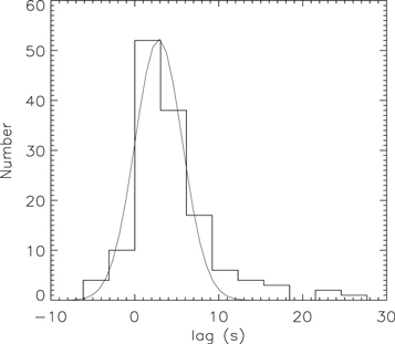
Figure 1. Distribution histogram of 137 flare lags, where the solid curve is the Gaussian fitting curve.
Download figure:
Standard image High-resolution imageIt is worth mentioning that the spectral lag in the prompt-emission pulse is mainly concentrated in the range of 10−2–10−1 s (Yi et al. 2006; Hakkila et al. 2007; Li et al. 2012b), while the lag of the flare is mainly concentrated in a few to tens of seconds; this shows that the lag of X-ray flares is much longer than that of prompt-emission pulses.
3.2. Lag–Duration Relation
The previous section shows that the flare lag is much greater than that of the prompt-emission pulse. There is a positive correlation between lag and pulse duration in gamma-ray prompt emission as revealed by many authors (e.g., Norris et al. 2005; Peng et al. 2007; Li et al. 2012b). Does the duration of the flare also have a great influence on the spectral lag? Figure 2 shows the correlation between the flare duration and the lag of the X-ray flare. The open circles are the 114 flares that show positive lag (we refer to these 114 flares showing positive time lag as sample 1), and the solid line is the best-fit relationship between the lag and duration of the flare: δ T = 101.81 ± 0.04, lag = 0.54 ± 0.06; the Spearman correlation coefficient is 0.60 with p = 1.19 × 10⁻¹². Previous studies have shown that the GRB prompt-emission pulse duration is also positively correlated with the spectral lag (e.g., Norris et al. 2005). Both the gamma-ray prompt-emission pulse and the X-ray flare have a consistent lag and duration correlation; their spectral lag is positively related to the duration. That is, the longer the duration, the greater the lag. The duration of the prompt-emission pulse is concentrated in a few seconds to tens of seconds, while the average duration of the flare in our sample 1 is 185.5 s. Since the flare has a longer duration, the lag of the flare is also greater.
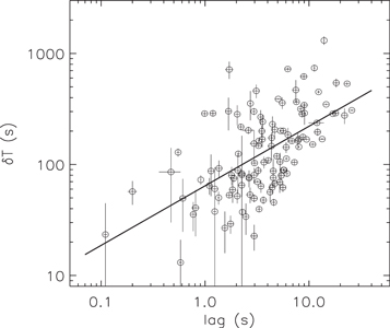
Figure 2. Best-fit relationship between flare lag and flare duration: δ T = 101.81 ± 0.04, lag = 0.54 ± 0.06; the Spearman correlation coefficient r is 0.6 with p = 1.19 × 10⁻¹².
Download figure:
Standard image High-resolution image3.3. The Evolution of Spectral Lag in Multiflare GRBs
Margutti et al. (2010) showed that X-ray flares evolve with time with a sample including nine single flares. That is, flares become wider as time proceeds, with larger peak lags. Moreover, they found that a single flare has the same width–lag correlation as a prompt-emission pulse; the wider the flare/pulse, the greater the lag value. Employing a much larger multiflare sample we also investigate the two issues.
Figure 3 demonstrates the flare spectral lag versus the flare peak time tpeak for sample 1; the black filled circles are the 114 flares that show positive lags, and the solid line is the best regression line. The best functional form of this relation is log( (A is in units of seconds). A correlation (Spearman correlation coefficient r = 0.34) is identified, with A = 2.26 ± 0.04 and B = 0.26 ± 0.06. Figure 4 plots the flare peak time and the duration of the flare; the solid line is the best-fitting line: tpeak = 101.62 ± 0.13, δ
T = 0.37 ± 0.06; the Spearman correlation coefficient is 0.45 with p = 4.13 × 10⁻⁷. These results are consistent with previous studies (e.g., Margutti et al. 2010). But both power-law indices of our sample are much smaller that those of Margutti et al. (2010). Therefore, in the case of multiflare GRBs, the flares also evolve with time, that is, the later the flares appear, the longer the durations and the larger the spectral lags.
(A is in units of seconds). A correlation (Spearman correlation coefficient r = 0.34) is identified, with A = 2.26 ± 0.04 and B = 0.26 ± 0.06. Figure 4 plots the flare peak time and the duration of the flare; the solid line is the best-fitting line: tpeak = 101.62 ± 0.13, δ
T = 0.37 ± 0.06; the Spearman correlation coefficient is 0.45 with p = 4.13 × 10⁻⁷. These results are consistent with previous studies (e.g., Margutti et al. 2010). But both power-law indices of our sample are much smaller that those of Margutti et al. (2010). Therefore, in the case of multiflare GRBs, the flares also evolve with time, that is, the later the flares appear, the longer the durations and the larger the spectral lags.
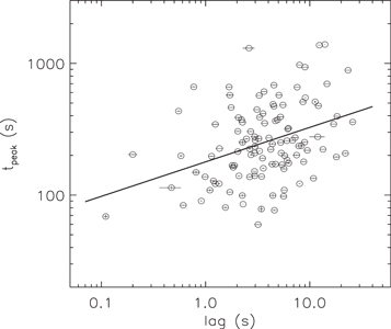
Figure 3. Best-fit relationship between lag and tpeak:  ; the Spearman correlation coefficient r is 0.34 with p = 1.75 × 10⁻⁴.
Download figure:
Standard image High-resolution image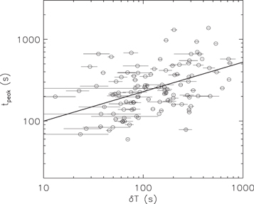
Figure 4. Best-fit relationship between duration and tpeak:  ; the Spearman correlation coefficient r is 0.45 with p = 4.13 × 10⁻⁷.
Download figure:
Standard image High-resolution image3.4. The Effect of Spectral Evolution Trends on the Multiflare GRB Lag
As mentioned above, there are 13 multiflare GRBs whose time lags show opposite signs. In order to study the causes of positive and negative lags, we select GRB 060714 and GRB 060111A to compare their spectral evolution trends since some scholars think that the spectral evolution may be causing the spectral lag (e.g., Kocevski & Liang 2003; Roychoudhury et al.2014). The light curves of the WT models of GRB 060714 and GRB 060111A are shown in the left panel of Figure 5. Both GRB 060714 and GRB 060111A have three obvious flares, which have complete structures and are very bright. We use the DCF to estimate the lags. The first and second flares of GRB 060111A and GRB 060714 show positive lags, while both of the third flares show negative lags (see Table 2). The third flares of these two GRBs have the longest duration and are relatively bright, so we choose these two GRBs to study the effect of spectral evolution on lags.

Figure 5. Left panels: The light curves of GRB 060111A and GRB 060714. Right panels: Time evolution of the peak energy from the time of flare peak for GRB 060111A and GRB 060714.
Download figure:
Standard image High-resolution imageTable 2. Fitting Results of the COMP Model and Band Model to GRB 060714 and GRB 060111A
| GRB | Flare | t1 (s) | t2 (s) | CPL | Band | ΔBIC | |||||||
|---|---|---|---|---|---|---|---|---|---|---|---|---|---|
| α | Ep (keV) | BIC | α | β | Ep (keV) | BIC | |||||||
| 060714 | 1 | 113 | 115 |

|

| 40.24 |

|

|

| 47.58 | 7.34 | ||
| 060714 | 1 | 115 | 117 |

|

| 64.79 |

|

|

| 72.69 | 7.9 | ||
| 060714 | 1 | 117 | 119 |

|

| 34.42 |

|

|

| 41.09 | 6.68 | ||
| 060714 | 1 | 119 | 121 |

|

| 52.89 |

|

|

| 59.83 | 6.94 | ||
| 060714 | 2 | 140 | 144 |

|

| 95.94 |

|

|

| 109.76 | 13.83 | ||
| 060714 | 2 | 144 | 150 |

|

| 104.6 |

|

|

| 113.3 | 8.71 | ||
| 060714 | 2 | 150 | 154 |

|

| 32.98 |

|

|

| 45.74 | 12.76 | ||
| 060714 | 2 | 154 | 159 |

|

| 56.82 |

|

|

| 67.24 | 10.41 | ||
| 060714 | 3 | 175 | 180 |

|

| 84.16 |

|

|

| 85.79 | 1.63 | ||
| 060714 | 3 | 180 | 184 |

|

| 72.33 |

|

|

| 78.09 | 5.76 | ||
| 060714 | 3 | 184 | 190 |

|

| 45.26 |

|

|

| 50.95 | 5.69 | ||
| 060714 | 3 | 190 | 195 |

|

| 33.38 |

|

|

| 39.69 | 6.31 | ||
| 060714 | 3 | 195 | 200 | ⋯ | ⋯ | ⋯ | ⋯ | ⋯ | ⋯ | ⋯ | ⋯ | ||
| 060714 | 3 | 200 | 235 |

|

| 47.06 |

|

|

| 56.07 | 9.02 | ||
| 060111A | 1 | 99 | 109 |

|

| 78.39 |

|

|

| 81.98 | 3.59 | ||
| 060111A | 1 | 109 | 118 |

|

| 99.3 |

|

|

| 103.86 | 4.56 | ||
| 060111A | 1 | 118 | 129 |

|

| 63.27 |

|

|

| 71.58 | 8.31 | ||
| 060111A | 1 | 129 | 139 |

|

| 67.42 |

|

|

| 76.46 | 9.04 | ||
| 060111A | 2 | 167 | 175 |

|

| 66.38 |

|

|

| 74.28 | 7.91 | ||
| 060111A | 2 | 175 | 186 | ⋯ | ⋯ | ⋯ | ⋯ | ⋯ | ⋯ | ⋯ | ⋯ | ||
| 060111A | 2 | 186 | 195 |

|

| 44.6 |

|

|

| 51.19 | 6.59 | ||
| 060111A | 2 | 195 | 201 |

|

| 24.98 |

|

|

| 31.28 | 6.3 | ||
| 060111A | 3 | 283 | 302 |

|

| 220.69 |

|

|

| 221.64 | 0.95 | ||
| 060111A | 3 | 302 | 323 |

|

| 318.14 |

|

|

| 295.71 | –22.42 | ||
| 060111A | 3 | 323 | 342 |

|

| 255.67 |

|

|

| 255.86 | 0.19 | ||
| 060111A | 3 | 342 | 363 |

|

| 140.69 |

|

|

| 147.49 | 6.8 | ||
| 060111A | 3 | 363 | 403 |

|

| 98.71 |

|

|

| 104.75 | 6.03 | ||
| 060111A | 3 | 403 | 432 |

|

| 74.75 |

|

|

| 81.09 | 6.34 | ||
| 060111A | 3 | 432 | 451 |

|

| 48.8 |

|

|

| 55.44 | 6.64 | ||
| 060111A | 3 | 451 | 510 |

|

| 101.22 |

|

|

| 107.15 | 5.93 | ||
Download table as: ASCIITypeset image
To examine whether spectral evolution is responsible for the observed spectral lags of GRB 060714 and GRB 060111A, we study the time variation of Epeak (the peak energy in the ν Fν spectrum) for all flares of GRB 060714 and GRB 060111A under consideration since the two GRBs have the most flares. In the spectral evolution of prompt-emission pulses, Epeak is often used to represent the process of spectral evolution; in X-ray afterglow flares, we also use the trend of Epeak to represent spectral evolution. Several theoretical models have been proposed to explain its wide distribution from several kiloelectronvolts to megaelectronvolts (Sakamoto et al. 2009; Roychoudhury et al. 2014).
We divide the attenuation time of all flares for the two GRBs into several time periods; the XRT data energy range is 0.3–10 keV. We extract the spectra for each time period from the Swift website (https://www.swift.ac.uk/) and then adopt the Multi-mission Maximum Likelihood Framework (3ML; Vianello et al. 2015) to fit the flare spectral data. The 3ML tool adopts the Markov Chain Monte Carlo (MCMC) technique to perform time-resolved spectral fitting. The MCMC technique is based on the Bayesian statistic using the 3ML tool to carry out parameter estimation of data. In order to choose a better model to fit the energy spectrum, we fit the flare spectral data with the BAND model (Band et al. 1993) and the COMP function (Mukherjee et al. 1998) to perform time-resolved spectral analysis and compare the ΔBIC of the BAND model and COMP model. ΔBIC is BICBAND − BICCOMP and ΔBIC greater than zero indicates that the COMP model is better. Then we check all cases and find that all ΔBIC are positive except one. The BAND model does not fit our energy spectrum well and the COMP model is the preferred model, since it systematically has a lower BIC value. Therefore, we mainly adopt the data from the COMP model in addition to one from BAND to analyze Epeak evolution with flare peak time. For the specific definition of the goodness of data fitting by the empirical model, please refer to Yu et al. (2019). The fitting results are shown in Table 2.
The COMP model is a single-power-law model with a high-energy cutoff, and the function form is as follows:

A is the normalization constant of the spectrum, α is the photon spectrum index, Ec
is the break energy in the spectrum, and Epeak and Ec
have such a relationship:  . This function fits all the flares of GRB 060714 and flares 1 and 3 of GRB 060111A very well; the floating point is not enough in the second-flare fitting energy spectrum of GRB 060111A, so we remove it. In GRB 060714, the first flare is a composite flare, which is relatively obvious in the 0.3–1.5 keV energy channel; this may have an impact on the evolution of Epeak.
Some scholars think that the spectral evolution from hard to soft causes the spectral lag (e.g., Kocevski & Liang 2003). Roychoudhury et al. (2014) suggested spectral evolution will cause both positive and negative lags; the evolution from hard to soft causes a positive lag, while the evolution from soft to hard causes a negative lag. A comparison of the time variations of Epeak for GRB 060111A and GRB 060714 is given in Figure 5.
The first and third flares of GRB 060111A show a positive lag and negative lag, respectively. The Epeak evolution trends of these two flares are not the same. The Epeak of the first flare of GRB 060111A has a hard-to-soft trend. However, the Epeak evolution of the third flare of GRB 060111A does not have a clear trend from soft to hard, but has a weak soft-to-hard-to-soft trend near the peak of the flare. This soft-to-hard-to-soft trend may be the cause of the negative lag in the third flare of GRB 060111A. This may be reasonable since Peng et al. (2011) also justified that the spectral evolution trend from soft to hard to soft in prompt-emission pulses will cause a negative lag.
In GRB 060714, a mixed flare appeared at the tail of the first flare. This may be the reason why this flare has a hard-to-soft-to-hard trend. The second flare and the third flare have similar hard-to-soft evolution trends, but their lags show opposite signs: the second flare shows a positive lag, whereas the third flare shows a negative lag. Thus it seems that spectral evolution is not the dominant cause of the spectral lag features of GRB 060714.
Spectral evolution has long been considered as the cause of spectral lag (e.g., Kocevski & Liang 2003). However, many studies have used different considerations to support the observation that spectral evolution may not be the dominant process responsible for the spectral lag of all GRBs (e.g., Ukwatta et al. 2012; Roychoudhury et al. 2014; Chakrabarti et al. 2018). We also think that spectral evolution cannot explain all spectral lags; there may be other physical mechanisms.
4. Discussion
The calculation accuracy of the spectral lag is related to the time resolution of the light curve and the signal-to-noise ratio. The CCF method is commonly used to calculate the lag of prompt-emission pulses. However, for XRT data, discrete data leads us to use the DCF to estimate flare lags. In order to verify the accuracy of this method for lag estimation, we compare the lag of GRB 060904B with that of the method used by Margutti et al. (2010) by fitting the two identical light curves. We first set the minimum signal-to-noise ratio to 4, then extract the light-curve data of the 0.3–1 and 2–3 keV energy channels, and estimate the lag of this GRB with the DCF. The DCF curve of GRB 060904 is shown in Figure 6, in which the red curve is the Gaussian fitting curve, the d used for the Gaussian curve peak pair is 2.87, the average time interval (Δt) is 8.3 s, and the corresponding lag is 23.8 s. Figure 1 of Margutti et al. (2010) shows that the lag of GRB 060904B between the 0.3–1 and 2–3 keV energy channels is also about 23 s. This shows that it is feasible to use the DCF to estimate the flare lag.

Figure 6. The DCF curve of GRB 060904B; the red solid curve is the Gaussian fitting curve.
Download figure:
Standard image High-resolution image4.1. Comparison of the Lag Properties of Multiflare GRBs and Multipulse GRBs
We choose 37 multipulse GRBs (including 88 pulses) from Li et al. (2012b) to check if there are similar lag properties between multiflare and multipulse GRBs. The lags of these 88 pulses are obtained by fitting the Gaussian model to the CCF curve, which is similar to the DCF method. The duration δ T of the pulse is also defined by δ T = Tend − Tstart; for more details, please refer to Figure 3 in Li et al. (2012b).
Figure 7 is the lag distribution of the 88 pulses: the pulse lags are between 50–100 and 15–25 keV, the red curve is the Gaussian fitting curve, the lags of the 88 pulses have a distribution similar to a Gaussian distribution, and the average value of this Gaussian distribution is about 0.18 s. In order to pick out the positive and negative lags we remove eight pulses with very large errors. Among the 80 remaining pulses, there are 68 positive-lag pulses (85%) and 12 negative-lag pulses (15%). Of the 68 positive-lag pulses, the median value is 0.27 s with a mean of 0.36 s. The pulse lags are much shorter than the flare lags, which may be caused by the fact that the durations of the pulses are much shorter than those of the flares.
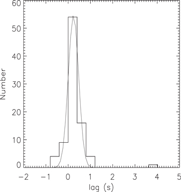
Figure 7. Histogram distribution of 88 pulses. The solid curve is the Gaussian fitting curve.
Download figure:
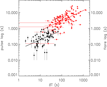
Standard image High-resolution imageFigure 8 shows the relationship between the lag and duration of the pulses/flares: the red filled circles on the right axis are the 114 flares, the black filled circles on the left axis are the 68 pulses, and the red solid line with associated slope 0.63 ± 0.08 and the black solid line with associated slope 0.60 ± 0.13 are the best-fit relationships for the flare lag and flare duration and for the pulse lag and pulse duration, respectively. Moreover, the slopes of the two relationships are very similar. From this perspective, multiflare GRBs and multipulse GRBs have similar characteristics (flares are an extension of pulses), which also provides support for X-ray flares and gamma-ray pulses having the same physical origin.
Figure 8. The black filled circles are the 68 pulses (from Li et al. 2012b), and the red filled circles are the 114 flares (from Yi et al. 2016). The red and black solid lines are the best-fit relationships between flare lag and flare duration and between pulse lag and pulse duration, respectively.
Download figure:
Standard image High-resolution image
4.2. The Possible Origin of the Spectral Lag of Multiflare GRBs
There are several phenomena responsible for the observed spectral lags, such as the curvature effect (Ryde & Petrosian 2002), the internal cooling of radiated electrons (Kazanas et al. 1998; Schaefer 2004), the Compton reflection of a medium far away from the radiation source, and the spectral evolution (Kocevski & Liang 2003) during the prompt phase. Mochkovitch et al. (2016) believe that spectral lag depends on all spectral changes including the pulse peak energy and spectral index. Spectral evolution means that as the energy dissipates, the radiation gradually cools down, and the overall trend of the energy spectrum moves toward low energy, which leads to mainly high-energy photons at the beginning, and fewer low-energy photons. After a period of radiation, the photons can fall to the low-energy channel, resulting in a positive lag of high-energy photons arriving first and low-energy photons arriving later. At a certain stage, if the central engine injects energy to accelerate the shell, it causes the energy spectrum to go from low energy to high energy and creates a negative lag.
The curvature effect causes low-latitude photons to arrive first and high-latitude photons to arrive later, and the smaller Doppler factor of high-latitude photons makes these photons fall to a lower-energy range, which causes low-energy photons to arrive later and form a positive lag. Peng et al. (2011) also proposed that spectral lag is a result of the combined actions of the spectral evolution and the curvature effect. The curvature effect always provides the contribution of positive lag, and the spectral evolution provides different contributions of positive and negative lags according to the evolution model of the spectrum. The inherent cooling of radiating electrons means that low-energy radiation will be generated later than high-energy radiation, hence a positive lag; the Compton reflection of a medium follows the same principle.
We also examine if the spectral evolution can explain the spectral lag of a flare. The spectral lag may be related to the peak energy characteristics of the flare. The spectral evolution near the peak of the third flare of GRB 060111A shows a weak soft-to-hard-to-soft trend, which may be the reason for the negative lag of this flare. Both the first and second flares of this GRB have positive lags. But the Epeak evolution models have opposite characteristics: the first flare follows the hard-to-soft evolution mode and the second one shows a soft-to-hard trend. So we suspect that the curvature effect (and the hard-to-soft spectral evolution) and the soft-to-hard-to-soft spectral evolution together affect the GRB, causing the time lags of this GRB to show opposite signs.
In GRB 060714, the second and third flares have similar hard-to-soft spectral evolution trends, but their lags have opposite signs; the spectral evolution cannot explain this phenomenon. This requires a new mechanism to explain the cause of the lags in the GRB. Inverse Compton scattering of low-energy thermal photons by relativistic electrons is one of the feasible schemes for GRB radiation, which may introduce a negative lag (Roychoudhury et al. 2014). The first and the second flares of GRB 060714 have positive lags, which may be affected by curvature effects (and positive spectral evolution), and the third flare has negative lags, which may be caused by inverse Compton scattering of low-energy thermal photons by relativistic electrons. But this is just our guess, and more detailed theoretical research is needed to explain it.
The reason for the two GRBs having opposite-sign lags may be the combined effect of curvature effect, spectral evolution, and inverse Compton effect. The number of negative lags is relatively small after all, and the curvature effect (and hard-to-soft spectral evolution) may be dominant in X-ray flares. More detailed theoretical studies are needed for either the prompt-emission pulses or the X-ray flares. We hope that there will soon be a complete theory to explain the relationship between the spectral lag and spectral evolution in GRBs, so that we can have a deeper understanding of the pulses/flares of GRBs.
Using the observations of the Swift Burst Alert Telescope and the Suzaku wide-area monitor, Roychoudhury et al. (2014) found the multipulse GRB 060814 has a similar phenomenon. They found that the spectral lags of the first two and fourth pulses are positive but the third pulse exhibits a negative lag. However, the time variations of the Epeak of all the pulses show the same trend. The similar phenomenon seems to also support the observation that flares and pulses have the same physical origin.
Most studies of spectral lag have focused on the evolution of the spectrum and the curvature effect. Hakkila et al. (2018b) put forward the theory that the presence of pulse/flare "structures" can explain why some pulses/flares exhibiting hard-to-soft evolution have negative lags while others have positive ones. They demonstrated negative lags can be created by spectrally evolving bumps in GRB pulse light curves (see Figures 18(b) and 19 in their paper) even when the pulses in which they are found exhibit hard-to-soft evolution. Therefore, the presence of evolving pulse structures also supports the observation that the GRB central engine might be responsible, and points to times in the light curve when this might occur.
Hakkila et al. (2018a, 2018b) found that GRB pulse structures also exhibit temporal symmetries. In other words, structures observed during the pulse decay phase match structures in the rise phase, in reverse temporal order. This observation strongly suggests kinematic mechanisms (Hakkila et al. 2018b; Hakkila & Nemiroff 2019), which might be associated with energy fluctuations in the central engine (in the form of impactor waves), but might also result from heterogeneities in the developing jet or from structural fluctuations in the medium through which the jet expands. Therefore, the explained energy injection from the central engine is not the only mechanism capable of forming negative lags.
5. Conclusions
We obtain 48 multiflare GRBs from Swift/XRT and carry out a spectral lag study on 137 flares and come to the following conclusions:
- (1)We find that about 9.5% of the 137 flares have negative lags and 89.8% have positive lags when fluctuations are counted. The lag and duration of X-ray flares are greater than those of gamma-ray prompt-emission pulses. Multiflare GRBs have a lag–duration relationship consistent with that of multipulse GRBs, and the flares are an extension of the pulses.
- (2)We find that flare lags evolve over time in multiflare GRBs, which is consistent with the prompt-emission pulses.
- (3)We consider two multiflare GRBs with negative lags. It is found that the spectral evolution seems to be the cause of the negative lag of GRB 060111A. However, existing theories cannot explain GRB 060714, whose time lags show opposite signs. Inverse Compton scattering of low-energy thermal photons by relativistic electrons may be the cause of the negative lag, but this requires more in-depth theoretical support. However, in the multiflare GRBs, the majority of the flares show positive lags, so the curvature effect and positive spectral evolution may be the dominant model of the spectral lag. Moreover, the presence of pulse/flare structures is a possible explanation for the positive and negative lags.
Different flares in the same GRB have spectral lags with opposite signs, which are the same phenomena as those observed in previous multipulse GRBs. However, we cannot totally exclude the possibility that the lag of the pulse/flare is just due to intrinsic statistical fluctuations, but we can expect that other multiflare/pulse GRBs would also have similar features, which requires us to study more such GRBs. Therefore, the study of the spectral lag of multiflare GRBs and multipulse GRBs can help us better understand the physics of GRBs.
We would like to thank the anonymous referee for constructive suggestions to improve the manuscript. This work is supported by the National Natural Science Foundation of China (grants 11763009 and 11263006), the Key Laboratory of Colleges and Universities in Yunnan Province for High-energy Astrophysics, and the Natural Science Fund of Liupanshui Normal College (LPSSY201401).