


Abstract
We report nonlinear wave–wave coupling related to whistler-mode or electron Bernstein waves in the near-Sun slow solar wind with Parker Solar Probe (PSP) data. Prominent plasma wave power enhancements usually exist near the electron gyrofrequency (fce), identified as electrostatic whistler-mode and electron Bernstein waves (Malaspina et al. 2020). We find that these plasma waves near fce typically have a harmonic spectral structure and further classify them into three types identified by the characteristics of wave frequency and electric power. For short, we will call these type i, type ii, and type iii waves. The first (type i) is the quasi-electrostatic whistler-mode wave and its second harmonic, which resembles the quasi-electrostatic multiband chorus in the Earth's magnetosphere. The second (type II) is the pure electron Bernstein wave. The last (type iii) is an intermixture of whistler-mode and electron Bernstein waves, where the wave mode driven by the coupling between them was also detected. During the first five orbits of PSP, the type iii spectra have the largest occurrence rate, then the type i spectra. The type ii spectra are the rarest type of wave. Our study reveals that nonlinear wave–wave coupling in the solar wind may be as common as in the Earth's magnetosphere.
Export citation and abstract BibTeX RIS
1. Introduction
Whistler-mode waves and electron Bernstein waves are prevalent plasma waves in space, such as in the solar wind and in the Earth's magnetosphere (Helliwell 1967; Kennel et al. 1970; Horne et al. 1981; Zhang et al. 1998; Meredith et al. 2009; Wilson et al. 2010). Whistler-mode waves are right-hand polarized electromagnetic emissions falling within the frequency range of lower hybrid frequency to electron cyclotron frequency (fce) and they were some of the first observed in situ waves in the Earth's magnetosphere (Tsurutani & Smith 1974; Burtis & Helliwell 1969; Thorne 2010). Many previous observations have confirmed the existence of whistler-mode waves in the solar wind from ∼0.3 to ∼1 au, and they are typically quasi-parallel, narrowbanded, and have frequencies below 0.5fce (Lacombe et al. 2014; Stansby et al. 2016; Jagarlamudi et al. 2020). During the first two perihelion passes of the Parker Solar Probe (PSP), whistler-mode waves were observed during low-turbulence solar wind intervals. These waves have turned out to be quasi-electrostatic and have very high frequencies near fce (Malaspina et al. 2020). Whistler-mode waves are a promising candidate for the formation of the halo and strahl populations of electrons in the solar wind (Vocks et al. 2005; Vocks 2012; Kajdič et al. 2016; Tong et al. 2019; Agapitov et al. 2020; Cattell et al. 2021). Electron Bernstein waves, also known as electron cyclotron harmonic (ECH) waves, are electrostatic emissions observed between the harmonics of the electron cyclotron frequency. Electron Bernstein waves have been detected more commonly in Earth's magnetosphere than in the solar wind (Kennel et al. 1970; Fredricks & Scarf 1973). Recently, Malaspina et al. (2020) found electron Bernstein waves in the near-Sun solar wind using the PSP and suggested they may play a role in regulating the solar heat flux carried by electrons.
The nonlinear wave–wave coupling related to whistler-mode or electron Bernstein waves is very common in the Earth's magnetosphere (Ellis & Porkolab 1968; Harker & Crawford 1968; Gao et al. 2017). Instruments on board the THEMIS satellite detected whistler-mode waves with a second or even a third harmonic (i.e., multiband chorus); these originate from coupling between the electrostatic and magnetic components (or the electrostatic component itself; Gao et al. 2016, 2017). Observations also revealed that one whistler-mode wave can be coupled with one electron Bernstein wave or another whistler-mode wave (Gao et al. 2018b). However, such nonlinear wave–wave coupling related to whistler-mode or electron Bernstein waves has been never reported in the solar wind.
In this study, we report wave–wave coupling related to whistler-mode and electron Bernstein waves in the near-Sun solar wind recorded by PSP up to the present time (with further incursions of PSP to the closeness to the Sun, one expects new and heretofore unknown wave–wave interactions). We find that plasma waves near fce are always observed along with harmonic spectra, which can be further classified into three types. The first is the quasi-electrostatic whistler-mode wave and its second harmonic. This resembles the quasi-electrostatic multiband chorus in Earth's magnetosphere (Gao et al. 2016). The second is pure electron Bernstein waves. The third is the intermixture of whistler-mode and electron Bernstein waves, where the wave mode driven by the coupling between them is also detected. A full understanding of the nonlinear evolution of these waves may have potential importance to the electron dynamics of the solar wind.
2. Instruments and Data
Launched in 2018 August, PSP is a mission designed to explore the near-Sun plasma environment, eventually reaching as close as 9.86 solar radii (RS ) from the center of the Sun (Fox et al. 2016). The FIELDS (Bale et al. 2016) equipment suite on board PSP provides in situ measurements of the wave magnetic and electric fluctuations. The plasma data are obtained from the Solar Wind Electrons Alphas and Protons (SWEAP; Kasper et al. 2016) instrument suites. We used the PSP data during the first five orbits and the perihelion distance between 27.8 RS and 35.6 RS .
The AC power spectra are calculated for four different channels (electric and magnetic field channels), which are obtained from the FIELDS Digital Fields Board (Malaspina et al. 2016). In this paper we primarily utilized the AC power spectra of differential voltage V12 ( = V1 − V2), which covers the frequency range of ∼140 Hz to 75 kHz and has a high cadence of ∼0.87 s. The AC power spectra data are organized in 56 pseudo-logarithmically spaced frequency bins. The magnetic field data in RTN (radial-tangential-normal) coordinates at 4.58 Samples s−1 are used for the ambient magnetic field, provided by the Fluxgate Magnetometer (MAG) instrument of the FIELDS suite.
The proton distribution moments are provided by the sunward-facing Solar Probe Cup (SPC) Faraday cup instrument (Case et al. 2020). The bulk velocity of protons is used to indicate the solar wind velocity. The temperature of core electrons is estimated by fitting the electron velocity distribution, which is measured by the Solar Probe Analyzers Electrons (SPAN-E; Whittlesey et al. 2020) with a time resolution of ∼28 s. Following the method used by Moncuquet et al. (2020), the electron density is calculated from the Quasi-thermal Noise (QTN) spectrum.
3. Observations
Figure 1 presents the solar wind conditions for three time intervals, including the ambient magnetic field (first row), solar wind velocity (second row), electron density (third row), and electron core temperature (bottom row). The periods that we are interested in, during which the harmonic spectra around the fce are detected, have been shaded in light green. The location of Event 3 is closest to the Sun, i.e., ∼36.6 RS , and Events 1 and 2 are observed at ∼36.9 and ∼38.2 solar radii (RS ), respectively. All three events are captured during low-turbulence periods with the near-radial ambient magnetic fields (Figures 1(a), (e), and (i)). The ambient solar wind magnetic field is disturbed before and after the wave intervals (shaded regions), but is significantly less disturbed during the wave intervals. This is consistent with the statistical result in Malaspina et al. (2020), where they suggested that the near-radial solar wind magnetic field with weak magnetic field turbulence may be a potential condition for the presence of these near—fce waves. The three events all occur in slow solar winds, i.e., the solar wind velocity is less than 450 km s−1 (Figures 1(b), (f), and (j)). The background plasma density is usually very high (Figures 1(c), (g), and (k)), and the ratios of the plasma frequency to electron gyrofrequency for three events are estimated as ∼41, ∼73, and ∼69, respectively. Thus the plasma beta is quite low, β ≤ 0.075 for the three events.
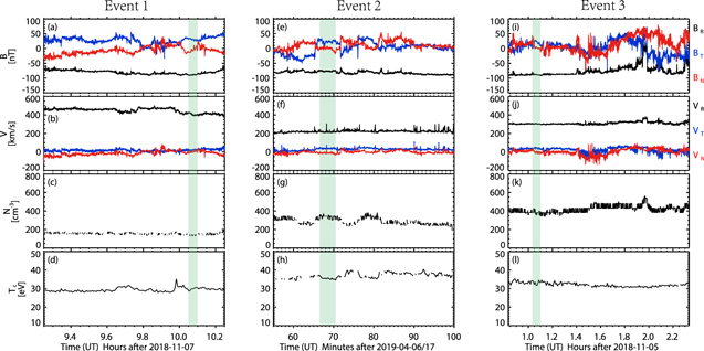
Figure 1. Solar wind conditions for three events. (a) The ambient magnetic field vector in RTN coordinates, (b) proton velocity in RTN coordinates, (c) electron density, and (d) electron core temperature for Event 1. (e)–(h) for Event 2. (i)–(l) for Event 3. The green shaded region marks the time interval when plasma waves are observed.
Download figure:
Standard image High-resolution imageUsing the wave frequency and spectral characteristics, we have found three types of electric spectra along with the harmonic structure around fce. The above three events are representative examples of the three types of harmonic spectra. The type i spectrum is displayed in Figure 2, which is observed during the time interval shaded in Figure 1(a). Figure 2(a) shows the spectrogram of differential voltage V12 from 10:03:45 to 10:06:30 UT, in which the white lines represent fce, 2fce, and 3fce, respectively. Two separated frequency bands exit in the spectrogram: one with a larger power, i.e., band 1, is located below fce (∼1831 Hz); the other is above fce (∼3662 Hz) and has a much lower power, i.e., band 2.
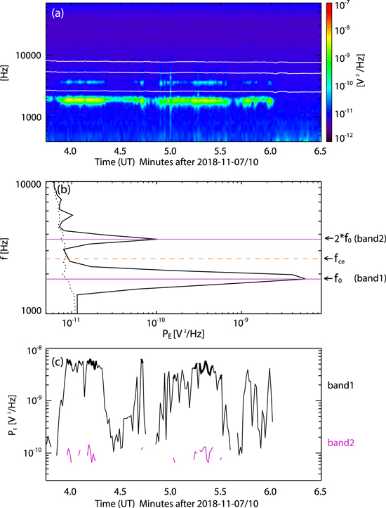
Figure 2. The type i spectrum. (a) Spectrograms of the differential voltage V12, (b) power spectral density PE vs. the frequency at 10:03:58 UT, and (c) peak power spectral densities PE for the whistler-mode wave (black) and its second harmonic (magenta). In panel a, solid white lines indicate the electron gyrofrequency fce and its harmonics. In panel b, the yellow dashed line marks the fce, and solid magenta lines represent the peak frequencies for two bands. The dotted black line denotes the background noise.
Download figure:
Standard image High-resolution imageWe present the electric power as a function of frequency at 10:03:58 UT in Figure 2(b), when band 1 has maximum wave power (5.7 × 10⁻⁹V2/Hz). In Figure 2(b), the peak frequency f0 with a dominant power for band 1 has been marked by the solid magenta line, along with its second harmonic 2f0, which coincides with the peak frequency of band 2 very well. We have also plotted the electric power around 10:06:20UT (without wave signal) as the background noise (dotted black line). Here we require that a valid wave signal have an electric power larger than the noise level.
Figure 2(c) shows the time profile of the peak wave power of valid wave signals for two bands. The thicker solid line (band 1) corresponds to the existence of band 2 (solid magenta line), suggesting that the second harmonic is excited only if the amplitude of the fundamental wave (band 1) reaches some threshold. It is found that the electric power of band 1 is typically 1–2 orders of magnitude larger than band 2. It is worth noting that there is no detectable wave signal near fce in the magnetic spectrogram during the same interval. For the type i event, we propose that band 1 is a quasi-electrostatic whistler-mode wave, and band 2 is the second harmonic driven by the nonlinear coupling of electrostatic components of band 1. This scenario is quite similar to the quasi-electrostatic multiband chorus in Earth's magnetosphere (Gao et al. 2018a).
Figure 3 presents the type ii spectra near fce, corresponding to the shaded time interval in Figure 1(e). The format of Figure 3 is the same as in Figure 2. In Figure 3(a), we find that there are four separated frequency bands lying on the electron gyrofrequency and its second, third, and even fourth harmonics. This is further exhibited in Figure 3(b). The electric power as a function of frequency at 18:06:51 UT is shown in Figure 3(b), where we have also marked the harmonics of the electron gyrofrequency (yellow dashed lines) and peak frequencies (fE1, fE2, fE3, and fE4) for the four bands (solid green lines). It is noted that the power peaks for the four bands are quite close to the first four harmonics of the electron gyrofrequency. Second, the power ratio between two adjacent frequency bands is usually less than one order of magnitude, which is also revealed in Figure 3(c), where the time profiles of the peak wave power of valid wave signals for all bands are presented. Again, we require that the electric power is at least one order of magnitude larger than the noise level (dotted black line) for a "valid" signal. The above observed properties of our type ii events are consistent with electron Bernstein waves. However, so far, we cannot tell whether the nonlinear wave–wave coupling is involved in type ii event generation solely based on the electric spectrogram.
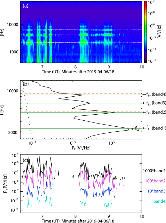
Figure 3. The type iii spectrum. (a) Same as Figure 2(a), (b) power spectral density PE vs. the frequency at 18:06:51 UT, and (c) peak power spectral densities PE for the first to fourth ECH wave bands (black, magenta, blue, and cyan). In panel a, solid white lines indicate the electron gyrofrequency fce and its harmonics. In panel b, the dashed yellow lines mark the electron gyrofrequency fce and its harmonics and the solid green lines represent the peak frequencies for four bands. The dotted black line denotes the background noise. In panel c, peak power spectral densities PE for the first to third wave bands are multiplied by 1000, 100, and 10.
Download figure:
Standard image High-resolution imageThe type iii spectrum near fce is shown in Figure 4, and this event occurs during the shaded time interval in Figure 1(i). In Figure 4(a), we can see there are several frequency bands found below and above fce. The spectrogram is not similar to that of event 1. Note that the wave spectra presented in Figures 3 and 4 show broadband wave power, while this broadband power is not observed in Figure 2. Statistically, the type i and type iii events usually show the narrow-band and broad-band power, respectively, while both narrow-band and broadband wave power is observed in type ii events. To identify which wave mode is involved in this event, we have presented the electric power as a function of frequency at 01:04:28 UT. We note that the frequency band f0 (∼0.66 fce; solid magenta line) is considered to be the quasi-electrostatic whistler-mode wave and its second harmonic 2f0 (magenta dash line) can also be observed. Second, the frequency bands (fE1 and fE2; solid green lines) close to fce and 2fce are identified as an electron Bernstein wave. This is consistent with the type ii spectrum. The most interesting feature is the frequency band marked by the blue line, whose frequency is just equal to the sum of the quasi-electrostatic whistler wave f0 and first electron Bernstein wave fE1. Its electric power is more than one order of magnitude smaller than either f0 or fE1. Figure 4(c) further displays the time profile of the peak wave power of valid wave signals for three bands, namely, f0, fE1 and f0 + fE1. The thicker solid line (band 1 and band 2) corresponds to the existence of band 3 (solid blue line). It is important to note that the frequency band f0 + fE1 can be observed only when both the f0 and fE1 bands have sufficiently large wave power. These properties suggest that the f0 + fE1 band is excited due to the nonlinear coupling between the quasi-electrostatic whistler wave and the electron Bernstein wave. Such coupling has also been reported to occur in the Earth's magnetosphere (Gao et al. 2018b). Thus the type iii wave event can be considered a mixture of whistler-mode and electron Bernstein waves and the nonlinear coupling between them.

Figure 4. The type iii spectrum. (a) Same as Figure 2(a), (b) power spectral density PE vs. the frequency at 01:04:28 UT, and (c) peak power spectral densities PE for the whistler-mode wave (black), ECH wave (magenta), and the coupling between the whistler-mode wave and the ECH wave (blue). In panel a, solid white lines indicate the electron gyrofrequency fce and its harmonics. In panel b, the magenta lines represent the peak frequencies for whistler-mode wave (solid) and its second harmonic (dash), the solid green lines represent the peak frequencies for the first two ECH wave bands, and the solid blue line represents the coupling between the whistler-mode wave and the ECH wave. The dotted black line denotes the background noise. In panel c, peak power spectral densities PE for band 1 and band 2 are multiplied by 1000 and 100.
Download figure:
Standard image High-resolution image4. Summary and Discussions
In this study, using PSP data, we have reported nonlinear wave–wave coupling related to whistler-mode and electron Bernstein waves in the near-Sun slow solar wind at a distance of ∼36.6 to ∼38.2 RS from the Sun. Based on the wave frequency and power, we found three types of electric spectra. The first is the quasi-electrostatic whistler-mode wave and its second harmonic, which resembles the quasi-electrostatic multiband chorus in the Earth's magnetosphere. The second is the pure electron Bernstein waves. The third is the mixture of whistler-mode and electron Bernstein waves. Note that the type iii wave events are similar to the wave event reported in Malaspina et al. (2021). Malaspina et al. (2021) examined the burst data of near-fce waves during a time interval of ∼3.5 s. In this study, we further find that nonlinear wave–wave coupling may also occur in type iii wave events.
Using the power spectra data obtained from PSP during the first five solar encounters, we have selected all wave events with frequencies near fce. First, we select the wave events by requiring that the sum of the power spectral density in the frequency range (0.3 fce−3 fce) at each point in time be greater than the threshold (4 × 10⁻¹⁰V2/Hz). Then, this data point (0.87 s) is counted as one wave event. We also visually inspected these events and remove some anomalous events and noise. Finally, we classify the three types of wave events through spectral characteristics. We have analyzed all the data during the first five encounters and the total time is ∼1460 hr. Figure 5 shows the percentage distribution of the three types of spectra. In total, ∼10 hr (∼41,400 time points) of data were found to include the type i spectrum (quasi-electrostatic whistler-mode wave and its second harmonic), ∼0.73 hr (∼3000 time points) of data including the type ii spectrum (pure electron Bernstein waves), and ∼34.7 hr (∼143,500 time points) of data including the type iii spectrum (the mingling of whistler-mode and electron Bernstein waves). We find that the type iii spectrum is most likely observed in the near-Sun solar wind. Based on previous theoretical studies (Ashour-Abdalla & Kennel 1978; Ashour-Abdalla et al. 1979; Neubert & Banks 1992; Menietti et al. 2002; Tripathi & Misra 2004), either the electron loss-cone distribution or an electron beam is unstable, which excites both the whistler-mode and electron Bernstein waves at the same time. To determine which electron distribution accounts for the wave spectrum near fce in the near-Sun solar wind requires in situ electron measurements with high time- and pitch angle- resolution. We will defer this for a future study.

Figure 5. The percentage distribution of three types spectra near the fce.
Download figure:
Standard image High-resolution image
Whistler-mode waves and electron Bernstein waves are widely detected in the Earth's magnetosphere. Both wave modes play key roles in regulating electron dynamics. Moreover, satellite observations show that various nonlinear wave–wave coupling processes exist that are related to whistler-mode or electron Bernstein waves in the magnetosphere. The statistical results also revealed that whistler-mode chorus and its harmonics (also called "multiband chorus") are very common phenomena. However, to our knowledge, such nonlinear wave–wave couplings have not been previously reported in interplanetary space. With the PSP data, we have found that the type i spectrum is quite similar to the quasi-electrostatic multiband chorus detected in the Earth's magnetosphere. The fundamental wave (f0) is below fce and the other wave occurs just lying on its second harmonic (2f0). The power ratio between the fundamental wave and its second harmonic is between one and two orders of magnitude, which is also similar with observations in the Earth's magnetosphere (Figures 3 and 8 in Gao et al. 2018a). In the type iii spectra, we also find a relatively weaker wave mode that could be driven by the coupling between the whistler-mode (below fce) and electron Bernstein waves. This has also been observed in the Earth's magnetosphere. Here we should mention that this wave mode may be too weak to be detected in some type iii spectra.
We therefore propose that nonlinear wave–wave couplings in the solar wind may be as common as in the Earth's magnetosphere, at least when one makes observations close to the Sun. Whistler-mode and electron Bernstein waves may play a crucial role in the evolution of the solar wind electron velocity distributions, and wave–particle interactions depend heavily on the spectral structure of plasma waves. Therefore, nonlinear wave–wave coupling related to whistler-mode or electron Bernstein waves may ultimately have some influence on the solar wind electron dynamics. The wave–wave coupling features noted in this paper taken at a distance of ∼37 RS from the Sun have not been noted in the solar wind closer to the Earth. It can be expected that even stronger coupling may be found as PSP orbits closer to the source of the solar wind, i.e., the Sun.
This research was funded by the Strategic Priority Research Program of the Chinese Academy of Sciences Grant No. XDB41000000, the NSFC grant 41774151, 41631071, USTC Research Funds of the Double First-Class Initiative (YD3420002001), the Fundamental Research Funds for the Central Universities (WK3420000013), and "USTC Tang Scholar" program. We also acknowledge the entire Parker Solar Probe team, and the data used in this study can be downloaded from spdf.gsfc.nasa.gov.