


Abstract
We present Atacama Large Millimeter/submillimeter Array CO (J = 2–1) and 1.3 mm continuum observations of the high-velocity jet associated with the FIR 6b protostar located in the Orion Molecular Cloud-2. We detect a velocity gradient along the short axis of the jet in both the red- and blueshifted components. The position–velocity diagrams along the short axis of the redshifted jet show a typical characteristic of a rotating cylinder. We attribute the velocity gradient in the redshifted component to rotation of the jet. The rotation velocity (>20 km s−1) and specific angular momentum (>1022 cm2 s−1) of the jet around FIR 6b are the largest among all jets in which rotation has been observed. By combining disk wind theory with our observations, the jet launching radius is estimated to be in the range of 2.18–2.96 au. The rapid rotation, large specific angular momentum, and a launching radius far from the central protostar can be explained by a magnetohydrodynamic disk wind that contributes to the angular momentum transfer in the late stages of protostellar accretion.
Export citation and abstract BibTeX RIS
1. Introduction
Protostellar jets are striking phenomena in star-forming regions and are considered to be an essential ingredient in the star formation process. Stars form in gravitationally collapsing clouds. The mass of a protostar at its birth is approximately a Jovian mass, or 0.1% the mass of the Sun (Larson 1969; Masunaga & Inutsuka 2000). After its birth, a protostar acquires additional mass by accreting material from a surrounding disk embedded in an infalling envelope. However, the rotation (or large angular momentum) of the disk prevents mass accretion onto the protostar from the circumstellar disk. Protostellar jets are believed to expel the excess angular momentum from the circumstellar region and allow accretion onto the protostar.
Observations of rotation in protostellar jets can be used to estimate the jet driving region assuming the Keplerian rotation of the circumstellar disk. In addition, we can identify the jet driving mechanism using the law of conservation of angular momentum (e.g., Mestel 1968). However, very high spatial resolution observations are necessary to measure jet rotation because protostellar jets are well collimated. Thus, jet rotation has been observed in only a limited number of cases. Since the first discovery of jet rotation (Bacciotti et al. 2002), several studies have observed rotation in protostellar jets (Launhardt et al. 2009; Bjerkeli et al. 2016; Chen et al. 2016; Lee et al. 2017; Tabone et al. 2017; Zhang et al. 2018). Recently, Hirota et al. (2017) clearly showed that rotation is present in the protostellar outflow driven by Orion Source I and estimated an outflow launching radius of >10 au from the central protostar. Their study suggests that protostellar outflows are directly driven from the intermediate region of the circumstellar disk by magnetohydrodynamics (see also Hirota et al. 2020).
In this study, we report the detection of fast rotating jets driven from the protostar FIR 6b (HOPS 60) in the Orion Molecular Cloud-2 (OMC-2; Mezger et al. 1990; Chini et al. 1997; Furlan et al. 2016). The jet rotation velocity exceeds 20 km s−1 and the specific angular momentum of the jet is as large as ∼1022 cm2 s−1, which hitherto is the largest value that has been observed in protostellar jets. The extraordinarily large rotation velocity and specific angular momentum can be explained by a magnetohydrodynamic disk wind (Blandford & Payne 1982). This is clear evidence that magnetic fields play a crucial role for protostellar evolution and that angular momentum is removed by protostellar jets.
FIR 6b is a Class 0 intermediate mass protostar (Chini et al. 1997; Takahashi et al. 2008; Furlan et al. 2016). The distance to FIR 6b is d ∼ 392 pc (Tobin et al. 2020) and the systemic velocity is vsys ∼ 11 km s−1 in the local standard of rest (LSR; Ikeda et al. 2007). FIR 6b has a bolometric luminosity of Lbol = 21.9 L⊙ (Furlan et al. 2016). A low-velocity (∼5 km s−1) bipolar outflow from FIR 6b extends from the northeast (blueshifted lobe) to the southwest (redshifted lobe) (Takahashi et al. 2008; Shimajiri et al. 2009). A small amount of gas remains in the envelope around FIR 6b (Chini et al. 1997; Shimajiri et al. 2009; Furlan et al. 2016). In addition, a disk-like structure with sizes of ∼126 and ∼56 au was also inferred from continuum observations at 0.87 mm by the Atacama Large Millimeter/submillimetre Array (ALMA) and 9 mm by the Very Large Array (VLA), respectively (Tobin et al. 2020). Thus, FIR 6b is expected to be in the late main accretion phase and considered to be a Class 0 protostar.
The structure of this paper is as follows. We describe the observations in Section 2. The observational results are presented in Section 3. We investigate the jet rotation and the driving mechanism in Section 4. The parameters and properties of the jets are described in Section 5. We discuss the effect of the inclination angle and the low-velocity component in Section 6. A summary is given in Section 7.
2. Observation
Mosaicking observations of the OMC-2/FIR 6 region in CO (J = 2–1; 230.538 GHz) and the 1.3 mm continuum were obtained with the ALMA 12 m array on 2018 April 19 and with the ACA 7 m array (Morita array) on 2018 January 7, 10, 11, and 17. The data were obtained through the Cycle 5 program 2017.1.01353.S (PI: S. Takahashi).
The mosaics cover a 3 8 × 39 area centered at (R.A., decl.) = (05h35m21s.7, −05°12'51
 0) with Nyquist sampling. In the 12 array and 7 m array observations, the mosaic consists of 108 and 42 pointings with an on-source integration time per pointing of 20 and 260 s, respectively. The overview of the full survey at OMC-2/FIR 6 region will be presented in a separate paper (Matsushita et al. in preparation 2021). In this paper, we present the results in the area centered on OMC-2/FIR 6b.
The correlator was configured to have four spectral windows, each observed in dual polarization mode. Two spectral windows were centered at 233.100 and 215.200 GHz with a bandwidth of 1875 MHz each to measure the continuum emission. The other two spectral windows were centered on CO (J = 2–1) and SiO (J = 5–4) with a bandwidth of 938 MHz and a spectral resolution of 244 kHz (0.64 km s−1 for CO J = 2–1). The SiO emission is not detected in FIR 6b. The arrays consisted of 44 and 11 antennas for the 12 m array and the 7 m array observations, respectively, with projected baseline coverage from 15.1 to 500.2 m and from 8.9 to 48.9 m. The FWHM primary beam size is 252 and 432, and the system temperatures ranged between 70 and 180 K and 60 to 210 K for the 12 m array and the 7 m array, respectively. The flux, gain, and bandpass calibrators were J0423-0120, J0541-0211, and J0423-0120 for the 12 m array, and J0522-3627 and J0607-0834, J0542-0913, and J0423-0120 for the 7 m array.
The data were calibrated using the Common Astronomy Software Application (CASA; McMullin et al. 2007), version 5.1.1, with the ALMA pipeline and imaged with CASA version 5.4.0. The CO line emission was separated from the continuum emission using "uvcontsub" task in CASA. The line-free regions in the CO and SiO spectral windows were combined with the two continuum windows to provide a total effective continuum bandwidth of 5.75 GHz.
The CO data from the 7 m array and the 12 m array were combined using the CASA task "concat" with a weight of 20:1. Only the ALMA 12 m array data were used to image of the 1.3 mm continuum emission. The CO and 1.3 mm continuum data were imaged by the CASA task "tclean" with a robust weight of 0.5. The primary beam correction was applied. The synthesized beam size of the CO cube has an FWHM size of 45 × 25 with a position angle of −87 0, and the continuum image has a beam size of 10 × 078 with the position angle of −736. The achieved noise levels are 30 mJy beam−1 for the CO image cube with a velocity resolution of 2.5 km s−1 and 0.5 mJy beam−1 for the 1.3 mm continuum image.
3. Results
Figures 1(a) and 1(b) show the integrated intensity and mean velocity maps of the low-velocity components (5–20 km s−1 with respect to the systemic velocity) toward FIR 6b. Cavity-like structures are seen in both ends of the redshifted and blueshifted jets in Figure 1(a). The moment 1 map (Figure 1(b)) shows both the redshifted (northeast) and blueshifted (southwest) components identified previously (Takahashi et al. 2008; Shimajiri et al. 2009). Blueshifted emission is detected between velocities of −20 and 10 km s−1, while redshifted emission is detected between 10 and 100 km s−1 (see Figure 1(c)). Figure 1(c) also shows that both the red- and blueshifted components contain two local emission peaks corresponding to the high-velocity components.

Figure 1. (a) CO (J = 2–1) integrated intensity map of the low-velocity component in the FIR 6b jet. The emission has been integrated between velocities of 0 and 30 km s−1, but excluding emission in the systemic velocities between 7.5 and 12.5 km s−1. The plus symbol at the center corresponds to the position of FIR 6b. The contour levels are at 5σ, 10σ, 15σ, and 20σ (1σ = 2.0 Jy beam−1 · km s−1). The black open ellipse in the bottom left corner indicates the synthesized beam. (b) Same as in panel (a), but for the mean CO (J = 2–1) velocity. The contours represent the integrated intensity shown in panel (a). (c) The CO (J = 2–1) line profile.
Download figure:
Standard image High-resolution imageFor the first time, we could confirm the high-velocity components (or high-velocity jets) driven from FIR 6b, which is distributed from the northeast to the southwest direction centered around FIR 6b as in the low-velocity components (Figure 1). Figure 2 shows the image of the high-velocity CO (J = 2–1) emission, in which the high-velocity components are integrated between 32.5 and 97.5 km s−1 for the redshifted jet, and between 17.5 and 0 km s−1 for the blueshifted jet. The red- and blueshifted components of the high-velocity emission are distributed in the same general direction as the low-velocity components (see Figure 1). The integrated high-velocity CO emission shows a well-collimated structure, within which several knots corresponding to local emission peaks indicated by arrows are embedded in the high-velocity jets.

Figure 2. CO (J = 2–1) integrated intensity map of the high-velocity component of the FIR 6b jet (color and black contours). The emission has been integrated over LSR velocities between 32.5 and 97.5 km s−1 (redshifted component, northeast side) and −17.5 to 0 km s−1 (blueshifted component, southwest side). The gray contours show the 1.3 mm continuum emission, which peaks toward OMC-2/FIR 6b at (R.A., Decl.) = (05h35m23s.34,  ). The synthesized beams are shown in the bottom left with a black open ellipse for the CO image and a filled gray ellipse for the 1.3 mm continuum image. The contour levels for the CO emission are at 5σ, 10σ, 15σ, and 20σ (1σ = 1.0 Jy beam−1 · km s−1). Contours for the 1.3 mm continuum emission are at 8σ, 40σ, 80σ, 120σ, 160σ, 240σ, and 320σ (1σ = 0.2 mJy beam−1).
Download figure:
Standard image High-resolution imageThe length of the jet, measured from the end of the blueshifted component to the end of the redshifted component, is ∼48,000 au. The jet width is ∼2400–5000 au depending on the distance from the central protostar. Although the CO emission in the southwest direction is slightly distorted near FIR 6b, the two components of the jet have a roughly symmetric structure around FIR 6b (Figure 2). The asymmetrical velocity structure in the upper- and lower-side of jets is sometimes seen in other observations (Matsushita et al. 2019). Recent simulations indicate that an asymmetrical jet (velocity) can be realized by the temporal asymmetric mass accretion from the infalling envelope onto the circumstellar disk (Matsumoto et al. 2017). The northeast side of the jet moves away from us with a velocity range of 22.5 to 87.5 km s−1 with respect to the systemic velocity, while the southwest side is coming toward us with a velocity of 10 to 27.5 km s−1 with respect to the systemic velocity. Thus, the northeast part corresponds to the redshifted component (or the redshifted jet), while the southwest part is the blueshifted component (or the blueshifted jet). The propagation direction of the high-velocity components is the same as that of the low-velocity components reported in previous studies (Takahashi et al. 2008; Shimajiri et al. 2009, see also Figure 1). Since the jets have a velocity range of 10 to 87.5 km s−1 with respect to the systemic velocity (Figure 1(c)), the intrinsic jet peak velocity might exceed 100 km s−1 after correcting for jet inclination angle (for details, see Section 5 and Section 6.1). However, the blueshifted jet has slower velocity than the redshifted one, and no high-velocity component has been observed in the southeast direction. This tendency has been shown in recent star formation simulations (Tsukamoto et al. 2020). In this paper, we mainly investigate the redshifted component to focus on the jet rotation in the high-velocity component.
Figure 3 shows maps of the mean velocity of the CO (J = 2–1) emission. A clear velocity gradient is found along the jet's short axis in the redshifted jet (Figure 3(a)). The northern part of the redshifted jet is moving toward the observer after the mean velocity is subtracted and the southern part is moving away from the observer. The velocity shifts along the minor axis by 25 to 50 km s−1. Thus, the redshifted jet seems to rotate around its long axis. Section 4 discusses alternative interpretations that could create a velocity gradient.
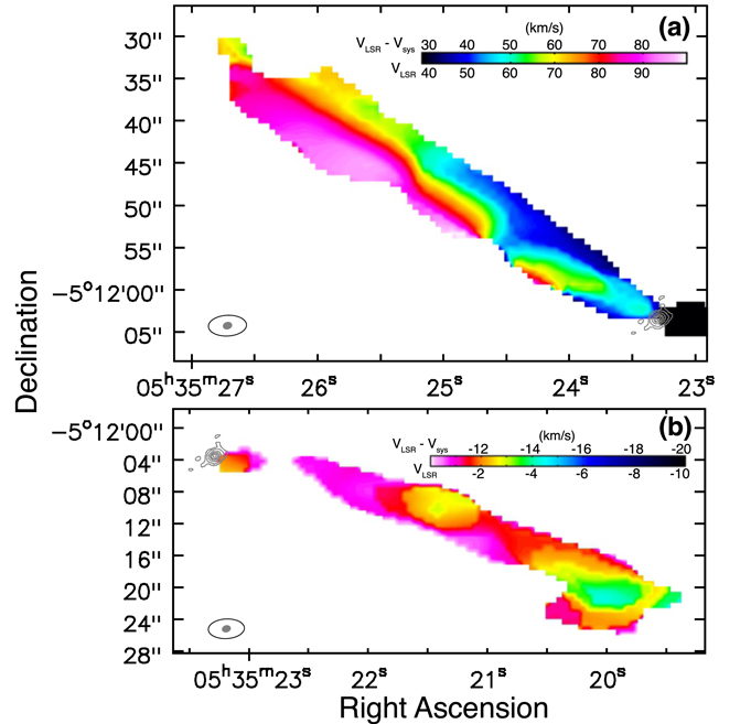
Figure 3. CO (J = 2–1) mean velocity maps of the FIR 6b jet. (a) Velocity map of the northeast side (redshifted) of the jet, computed for LSR velocities between 32.5 and 97.5 km s−1. (b) Velocity map of southwest side (blueshifted) of the jet, computed for LSR velocities between −17.5 and 0 km s−1. The 1.3 mm continuum emission is also plotted in each panel with gray contours as in Figure 2. The ellipses in the bottom left corner are the synthesized beams sized for the CO J = 2–1 (black) and the 1.3 mm continuum (gray) images.
Download figure:
Standard image High-resolution imageFigures 4 and 5 show the channel maps of the redshifted (northeast side) and blueshifted (southwest side) jets. In Figure 4, the jet axis is defined to pass through the emission peaks of the three knots at an LSR velocity of 70 km s−1. In the LSR velocity range of 30–70 km s−1, the emission peaks show a deviation from the jet axis in the northeast direction, while in the velocity range of 70–95 km s−1, the deviation from the jet axis is in the southwest direction. Although the velocity gradient depends on the distance from the position of FIR 6b, the emission peak is seen on both sides of the jet axis in the channel map. In addition, we can confirm three knots or relatively strong emission peaks in Figure 4. On the other hand, we cannot confirm the emission peak on both sides of the jet axis in the blueshifted jet (Figure 5).
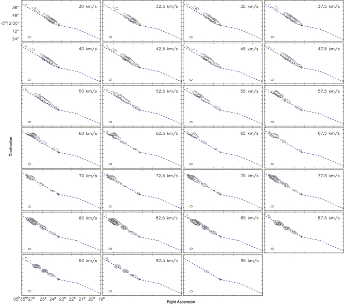
Figure 4. CO (J = 2–1) channel map of the redshifted flow from FIR 6b. The channel maps are presented in the LSR velocity range between 30 and 95 km s−1, which corresponds to the relative velocity range of 19 to 84 km s−1 with respect to the systemic velocity (vsys = 11 km s−1). The center value of the LSR velocity is indicated in each panel. The plus symbol at the center corresponds to the position of FIR 6b as measured in the 1.3 mm continuum image. The dashed lines indicate the axes of the redshifted (northeast side) and blueshifted (southeast side) jets. The jet axis of the redshifted components is determined from 70.0 km s−1 channel. The contour levels are 3σ, 5σ, 10σ, 15σ, 20σ, 30σ, 40σ, 60σ, 80σ, and 100σ (1σ = 30 mJy beam−1 · km s−1). The black open ellipse in the bottom left corner is the synthesized beam size.
Download figure:
Standard image High-resolution image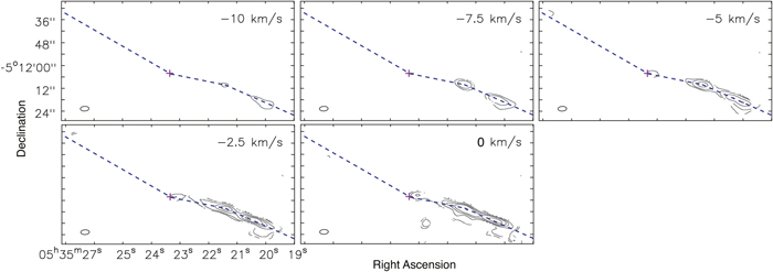
Figure 5. Same as in Figure 4 but for CO (J = 2–1) channel map of the blueshifted flow. The channel maps are presented in the LSR velocity range between −10 and 0 km s−1, which corresponds to the relative velocity range of −22 to −11 km s−1 with respect to the systemic velocity (vsys = 11 km s−1).
Download figure:
Standard image High-resolution imageFigure 6 shows position–velocity (PV) diagrams along the minor axis of the redshifted component. In Figure 6(b)–(e), there are two intensity peaks in the PV diagrams cutting along the short axis for each redshifted component at R1, R3, R7, or R9. The peaks are located in the second and fourth quadrants independent of the cutting position. The tendency seen in the PV diagrams agrees well with the typical characteristic of the rotating cylinder (Hirota et al. 2017). The PV diagrams for FIR 6b (Figure 3) do not agree with those seen in numerical simulations of a precessing jet (Raga et al. 2001; Masciadri et al. 2002). The two emission peaks would correspond to the wall or edge of the jet where the integrated intensity along the line of sight should be strong. In addition, the directions of velocity gradient are the same in all the cutting positions. This is natural if the velocity gradient is attributed to the jet rotation.
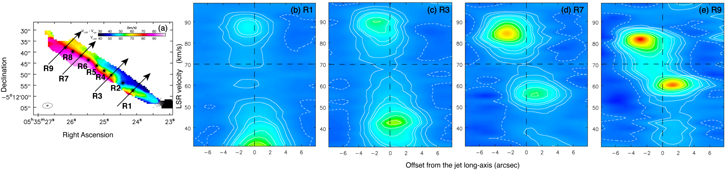
Figure 6. Position–velocity (PV) diagrams perpendicular to the long axis of the redshifted jet from FIR 6b. (a) The mean velocity map of the CO (J = 2–1) emission. R1–R9 indicate the slices of the PV diagram at 13'', 19'', 25'', 29'', 33'', 38'', 42'', 46'', and 49'' from the center of the 1.3 mm continuum emission. PV diagrams are shown for R1 (panel (b)), R3 (panel (c)), R7 (panel (d)), and R9 (panel (e)). The horizontal dashed line indicates the LSR velocity of 70 km s−1 (the center speed of jet rotation), while the vertical dashed line corresponds to the center of the jet axis denoted by the filled circles in panel (a). The contour levels are at -5σ, 5σ, 10σ, 20σ, 25σ, 50σ, 75σ, and 100σ (1σ = 10 mJy beam−1).
Download figure:
Standard image High-resolution image4. Jet Rotation and Other Possibilities
The velocity gradient detected in the redshifted component seems to be explained by the jet rotation, as described in Section 3. However, other mechanisms can also produce apparent velocity gradients, such as jet precession, twin jets, and asymmetrical jet structure (Chen et al. 2016). In this section, we discuss possible mechanisms that could cause the observed velocity gradient in the FIR 6b jet.
When a jet precesses, the velocity gradient tends to appear along the jet's long axis or the jet propagation direction. On the other hand, the jet velocity is not significantly changed along the jet's short axis in precession models (Raga et al. 2001; Masciadri et al. 2002). In addition, the precessing jet should have a strong wave-like structure as a whole (Masciadri et al. 2002), while the observed jet in FIR 6b is straight in both the redshifted and blueshifted lobes in the integrated intensity map (Figure 2). Moreover, as described in Section 3, the PV diagrams of the redshifted component are not in agreement with that derived in the precessing jet model (Raga et al. 2001; Masciadri et al. 2002).
If FIR 6b is a binary system, two protostars can drive two jets. In such a case, the velocity gradient (Figure 3(a)) can be potentially explained by twin jets if the directions of the jets differ slightly (Hara et al. 2021; Saiki & Machida 2020). It seems in fact that the redshifted jet splits along its long axis in the velocity map (Figure 3(a)). However, we cannot see any signature of the twin jets in the integrated intensity map (Figure 2). In addition, there is no evidence for a protobinary system in the 1.3 mm continuum image at 400 au spatial resolution (Figure 2) or in ALMA 0.87 mm and VLA 9 mm observations at 40 au resolution (Tobin et al. 2020). Thus, it is unlikely that the jet is composed of twin flows.
When the jet has an asymmetric or complex velocity distribution, the velocity gradient would appear in the jet's short axis. However, the distribution of CO emission is rather smooth (Figure 2) and the velocity gradient is systematic. Thus, the velocity gradients within the FIR 6b jet cannot be explained just by an asymmetric velocity distribution.
We conclude that rotation is the most plausible interpretation of the velocity gradient observed in the FIR 6b jet (Figure 3(a)). In addition, there are similarities between numerical simulations of protostellar jets and the observations. A winding configuration of velocity gradient seen in the velocity map can be seen in simulations of rotating jets (Staff et al. 2015). Further, the knots along the jet seen in the integrated intensity map (Figure 2) are also produced in simulations and can be explained by time-variable mass ejection (Machida & Basu 2019).
5. Derivation and Comparison of Jet Parameters
In this section, we derive the properties of the redshifted jet. Using the position–velocity diagram (Figure 6), the jet rotation velocity vϕ and the distance from the jet axis (or radius in the cylindrical coordinate) rrot are estimated as

and

respectively (Chen et al. 2016), where vblue and vred are the velocity at emission peak of the redshifted and blueshifted components in each PV diagram (Figure 6). The jet rotation axis was determined using the PV diagrams, in which the midpoint between the two emission peaks is adopted to define the jet axis. The jet width lshift was calculated as the distance between the two peaks in the PV diagrams.
Furlan et al. (2016) estimated a disk inclination angle of i = 80° with respect to the line of sight (Furlan et al. 2016). Using our 1.3 mm continuum data, we fitted a two-dimensional Gaussian to derive a deconvolved disk size of  (416 × 312 au), which implies an inclination angle of
  . Tobin et al. (2020) used higher angular resolution observations to derive a disk inclination angle of i = 55°. A recent theoretical study showed that the inclination angle of the disk (or normal direction of the disk) may change depending on the spatial scale (Machida et al.2020). Thus, it is difficult to accurately determine the inclination angle of the disk and jet from observations. Here, we adopt the jet inclination angle i = 80°, which gives the minimum rotation velocity and specific angular momentum (see Equation (1)). We discuss the dependence of the inclination angle on the jet properties in Section 6.1.
The measured rotation velocities are in the range of vϕ = 11.2–28.4 km s−1 , while the jet radius (or the distance from the jet axis) is in the range of rrot ∼ 220–800 au (Table 1). The rotation velocities estimated for FIR 6b are the highest among those reported in other sources even after correcting for the jet inclination angle: vϕ = 6–15 km s−1 for DG Tau (Bacciotti et al. 2002), ∼2 km s−1 for CB 26 (Launhardt et al. 2009), ∼5–14 km s−1 for SVS 13A (Chen et al. 2016), and ∼10 km s−1 for Orion Source I (Hirota et al. 2017).
Table 1. Physical Properties of the Jet for i = 80°
| Position | j | r0 | rrot | vϕ | vp | rA |
|---|---|---|---|---|---|---|
| (cm2 s−1) | (au) | (au) | (km s−1) | (km s−1) | (au) | |
| R 1 | 9.2 × 10²¹ | 2.18 | 216 | 28.4 | 344 | 25.7 |
| R 2 | 1.6 × 10²² | 2.79 | 440 | 23.9 | 364 | 40.5 |
| R 3 | 1.9 × 10²² | 2.96 | 529 | 23.9 | 381 | 46.4 |
| R 4 | 1.4 × 10²² | 2.53 | 480 | 19.3 | 367 | 35.4 |
| R 5 | 1.7 × 10²² | 2.78 | 700 | 16.2 | 379 | 41.9 |
| R 6 | 1.5 × 10²² | 2.35 | 549 | 18.8 | 410 | 35.3 |
| R 7 | 1.7 × 10²² | 2.60 | 760 | 15.2 | 402 | 40.3 |
| R 8 | 1.5 × 10²² | 2.32 | 800 | 12.2 | 402 | 34.0 |
| R 9 | 1.4 × 10²² | 2.16 | 804 | 11.2 | 407 | 31.0 |
Download table as: ASCIITypeset image
Given the inferred jet velocity and radius, the specific angular momentum of the jet at each position can be estimated as j = vrot × rrot. The specific angular momentum is in the range of 9.2 × 1021 cm2 s−1 ≤ j ≤ 1.9 × 1022 cm2 s−1 (Table 1). The maximum specific angular momentum estimated in this study is one or two orders of magnitude larger than those reported in other sources. The specific angular momenta calculated in previous studies are j ∼ 3.5 × 1020 cm2 s−1 for DG Tau (Bacciotti et al. 2002), ∼1.5 × 1020 cm2 s−1 for CB 26 (Launhardt et al. 2009), and ∼7.5 × 1020 cm2 s−1 for Orion Source I (Hirota et al. 2017). Among the jets where the rotation speed was measured, only the rotating jet bullet SVS 13A has a comparable but slightly smaller value of specific angular momentum (∼9.8 × 1021cm2 s−1) (Chen et al. 2016).
It is crucial to explore the launching radius r0 of the jet in order to clarify the jet driving mechanism. Based on Bernoulli's theorem and conservation of angular momentum, we can estimate the jet launching radius (Mestel 1968). Using the same method, the launching radius (r0) has been estimated as 10–100 au for low-velocity outflows (Alves et al. 2017; Hirota et al. 2017) and 0.05–7 au for high-velocity jets (Chen et al. 2016; Lee et al. 2017) in various objects. For FIR 6b, the launching radius is estimated using the toroidal vϕ and poloidal vpol velocities and the jet radius of each position with the analytical solution (Anderson et al. 2003)
where the poloidal velocity components of the jet are derived from

The mass of the central protostar is assumed to be Mstar = 1 M⊙. Note that the dependence of the estimated launching radius on the protostellar mass is weak (Equation (3)). The rotation velocity and radius estimated in the PV diagrams imply a jet launching radius in the range of r0 = 2.18–2.96 au (Table 1). When Mstar = 0.1 M⊙, then r0 = 1.01–1.38 au. Thus, the jet is expected to be driven by the intermediate region of the circumstellar disk where magnetic field is expected to be coupled with neutral gas (Machida & Basu 2019), not by the region very close to the protostar. Therefore, these observations are most consistent with the disk wind mechanism (Blandford & Payne 1982; Tomisaka 2002), where the jet is driven from a wide range of radii. The observations are inconsistent with the X-wind and entrainment mechanisms (Shu et al. 1994; Arce et al. 2007), in which the jet is driven from a region very close to the protostar (≲0.01 au). High-velocity jets with a small amount of angular momentum are expected in the X-wind and entrainment scenarios, because the jets appear in the region near the protostar where the angular momentum is not large.
The very large specific angular momentum of the FIR 6b jet cannot be easily explained. For example, the centrifugal radius is estimated as rcent = j2/(GMstar), inside which the Keplerian rotation is assumed. With j = 1022 cm2 s−1 and Mstar = 1M⊙, the centrifugal radius becomes rcent = 4.9 × 10⁴ au. The centrifugal radius estimated here is much larger than the disk-like structure observed around FIR 6b, and is not realistic. Thus, the jet needs to obtain a very large angular momentum through some other mechanism. The magnetic effect can provide a reasonable solution to the large specific angular momentum and the origin of the super-rotation of the jet.
To investigate the effect of magnetic field on the angular momentum transfer, the Alfvén radius rA (Anderson et al. 2003) at each position is estimated using

where  is the Keplerian angular velocity at the jet launching radius. The Alfvén radius is in the range of rA
= 25.7–46.5 au (Table 1). The ratio of the Alfvén radius to the jet launching radius (λ) is as large as λ ≡ rA
/r0 = 11.8–15.7. Thus, the long magnetic lever arm efficiently transports the angular momentum from the circumstellar region for the super-rotating jet case (Pudritz & Ray 2019).
is the Keplerian angular velocity at the jet launching radius. The Alfvén radius is in the range of rA
= 25.7–46.5 au (Table 1). The ratio of the Alfvén radius to the jet launching radius (λ) is as large as λ ≡ rA
/r0 = 11.8–15.7. Thus, the long magnetic lever arm efficiently transports the angular momentum from the circumstellar region for the super-rotating jet case (Pudritz & Ray 2019).
The magnetic pressure dominates the ram pressure within the Alfvén radius. Therefore, the large λ means that the magnetic field plays a dominant role near the protostar. The large lever arm is realized when the magnetic field threading the disk is strong and the mass loaded onto the wind (or the magnetic field line) is very small under which the jet can be accelerated to a large cylindrical radius before the magnetic field line is bent back by the plasma inertia. We expect such an environment is realized in a late main accretion phase during which the plasma beta (the ratio of thermal to magnetic pressure) above and below the disk is expected to be very low with a low-density and a strong magnetic field, and the wind mass is also very small (Machida & Hosokawa 2013).
Since the jet launching region is in the range of 2.18–2.96 au (Table 1), the foot points of the magnetic field lines connecting to the jet are also distributed in the same range of the circumstellar disk. Thus, wirelike strong (or hard) magnetic field lines originating in the circumstellar disk near the protostar (2.18–2.96 au) swing the fluid elements located very far from the foot points of the magnetic field lines (25.7–46.5 au). Since the fluid elements are frozen to the magnetic field lines, they are forced to corotate with the Keplerian velocity at foot points of the magnetic field lines, as seen in the schematic view of Figure 7. As a result, the fluid elements receive the angular momentum and are expelled from the circumstellar region by magnetic effect (Pudritz & Norman 1986). On the other hand, a parcel of gas in the circumstellar disk near the protostar loses the angular momentum and falls onto the protostar (Pudritz & Ray 2019). Therefore, the excess angular momentum is ejected from the circumstellar disk by the rotating jet, and the gas whose angular momentum has been removed by the jet falls onto the protostar and promotes the protostellar growth.

Figure 7. Schematic view of a super-rotating jet. The magnetic field line inside the Alfvén radius (thick dotted and solid red lines) rotates rigidly with the Keplerian velocity at its foot point and accelerates the gas elements located at the tip. The magnetic field line (red curve) is strongly twisted within the jet. The angular velocity of the jet is the same as that of the foot point and thus the super-rotation (blue arrows) is realized.
Download figure:
Standard image High-resolution image
6. Discussion
6.1. Effect of Jet Inclination Angle
The inclination angle of the jet is adopted as i = 80° when estimating the properties of the jet. However, as described in Section 5, the inclination angle of the disk is inferred to be i = 42° from our observations of the 1.3 mm continuum and i = 55° from published, higher angular resolution continuum observations (Tobin et al. 2020).
Since the jet physical quantities depend on the assumed inclination angle, Table 2 lists the jet properties for i = 40° and 60°. For these two cases, the specific angular momentum exceeds j = 1022 cm2 s−1, the maximum rotation velocity exceeds 40 km s−1, and the jet launching radius ranges between 4 and 13 au, which is considerably further from the star when assuming i = 80°. Therefore the adopted inclination angle does not significantly affect the conclusions. Thus, the distant launching radius and the rapid jet rotation inferred for the FIR 6b jet imply that the X-wind and entrainment scenarios are not the primary driving mechanisms. It should be noted that although the CO outflow discussed in this study supports the disk wind scenario, an X-wind component could still be present. If future observations identify a faster component with a small amount of angular momentum, it might correspond to the jet in the X-wind model. The disk wind and X-wind can coexist and contribute to the angular momentum transfer at different radii in the disk.
Table 2. Physical Properties of the Jet for i = 40 and 60°
| i = 40° | i = 60° | |||||||||
|---|---|---|---|---|---|---|---|---|---|---|
| Position | j | r0 | vϕ | vp | rA | j | r0 | vϕ | vp | rA |
| (cm2 s−1) | (au) | (km s−1) | (km s−1) | (au) | (cm2 s−1) | (au) | (km s−1) | (km s−1) | (au) | |
| R1 | 1.4 × 10²² | 20.1 | 43.6 | 78.3 | 169 | 1.0 × 10²² | 9.3 | 32.3 | 120 | 81.5 |
| R2 | 2.4 × 10²² | 26.6 | 36.6 | 82.9 | 272 | 1.8 × 10²² | 12.3 | 27.1 | 127 | 120 |
| R3 | 2.9 × 10²² | 28.3 | 36.6 | 86.8 | 313 | 2.2 × 10²² | 13.1 | 27.1 | 133 | 152 |
| R4 | 2.1 × 10²² | 24.2 | 29.6 | 83.5 | 238 | 1.6 × 10²² | 11.2 | 21.9 | 128 | 115 |
| R5 | 2.6 × 10²² | 26.7 | 24.9 | 86.1 | 284 | 1.9 × 10²² | 12.4 | 18.5 | 132 | 138 |
| R6 | 2.4 × 10²² | 22.5 | 28.8 | 93.3 | 238 | 1.8 × 10²² | 10.4 | 21.3 | 143 | 115 |
| R7 | 2.7 × 10²² | 24.9 | 23.3 | 91.4 | 272 | 2.0 × 10²² | 11.6 | 17.3 | 140 | 132 |
| R8 | 2.2 × 10²² | 22.2 | 18.7 | 91.4 | 229 | 1.7 × 10²² | 10.3 | 13.9 | 140 | 111 |
| R9 | 2.1 × 10²² | 20.6 | 17.1 | 92.7 | 208 | 1.5 × 10²² | 9.6 | 12.7 | 142 | 101 |
Download table as: ASCIITypeset image
6.2. Low-velocity Component
No clear velocity gradient is detected in either of the low-velocity components (Figure 1). The outflow (or jet) velocity should be proportional to the Keplerian velocity at the outflow driving radius. Thus, it is natural that rapid rotation is observed only in the high-velocity component, in which the base of the high-velocity outflow (or jet) is located near the protostar where the Keplerian rotation is high. The lack of a detectable velocity gradient in the low-velocity components may be attributed to a driving radius located relatively far from the central protostar where the Keplerian rotation velocity is small. Further high resolution observations are needed to confidently understand the driving mechanism of the jets.
7. Summary
We present high resolution ALMA observations of CO (J = 2–1) and the 1.3 mm continuum of the protostellar jet from the protostar FIR 6b in OMC-2. A clear velocity gradient is found along the short axis of the high-velocity, redshifted component of the jet. We attribute the velocity gradient to rotation. Using PV diagrams and an analytical model, the jet properties are inferred. The rotation velocity (>20 km s−1) and specific angular momentum (>1022 cm2 s−1) are extraordinarily large compared to previously observed jets. We suggest that the super-rotation of the jet is caused by the efficient transfer of angular momentum from the disk to the jet by magnetic fields. In addition, the jet launching points are inferred to be a radius of 2.18–2.96 au. These findings are consistent with the disk wind hypothesis as the primary jet driving mechanism for FIR 6b. The study could unveil the final phase of the protostellar evolution.
We thank the referee for very useful comments and suggestions on this paper. This work was financially supported by the Grants-in-Aid for JSPS Fellows (Y.M.). This paper makes use of the following ALMA data: ADS/JAO.ALMA#2017.1.01353.S. ALMA is a partnership of ESO (representing its member states), NSF (USA) and NINS (Japan), together with NRC (Canada), MOST and ASIAA (Taiwan), and KASI (Republic of Korea), in cooperation with the Republic of Chile. The Joint ALMA Observatory is operated by ESO, AUI/NRAO and NAOJ. The present study was supported by JSPS KAKENHI grants (JP21K03617, JP21H00046: MNM, and 19K03919: KY). Y.M. was supported by the ALMA Japan Research Grant of NAOJ ALMA Project, NAOJ-ALMA-255.