


Abstract
Collisionless shocks are some of the most efficient particle accelerators in heliospheric and astrophysical plasmas. Here we study and quantify ion acceleration at Earth's bow shock with observations from NASA's Magnetospheric Multiscale (MMS) satellites and in a global hybrid-Vlasov simulation. From the MMS observations, we find that quasiparallel shocks are more efficient at accelerating ions. There, up to 15% of the available energy goes into accelerating ions above 10 times their initial energy. Above a shock-normal angle of ∼50°, essentially no energetic ions are observed downstream of the shock. We find that ion acceleration efficiency is significantly lower when the shock has a low Mach number (MA < 6) while there is little Mach number dependence for higher values. We also find that ion acceleration is lower on the flanks of the bow shock than at the subsolar point regardless of the Mach number. The observations show that a higher connection time of an upstream field line leads to somewhat higher acceleration efficiency. To complement the observations, we perform a global hybrid-Vlasov simulation with realistic solar-wind parameters with the shape and size of the bow shock. We find that the ion acceleration efficiency in the simulation shows good quantitative agreement with the MMS observations. With the combined approach of direct spacecraft observations, we quantify ion acceleration in a wide range of shock angles and Mach numbers.
Export citation and abstract BibTeX RIS
1. Introduction
Collisionless shocks are abundant in astrophysical plasmas and are hosts to some of the most energetic plasma phenomena in the universe. Particles are accelerated by being scattered on both sides of the shock in a process known as diffusive shock acceleration (DSA) (Axford 1981). High-energy galactic cosmic rays are likely accelerated at supernova remnant shock waves through DSA (e.g., Morlino & Caprioli 2012). The Earth's bow shock is a place where ions are accelerated in DSA (e.g., Ellison & Moebius 1987). However, the maximum energy an ion can attain through DSA is expected to be limited at the bow shock. Kis et al. (2004) determined, using Cluster measurements, the spatial gradient of energetic ions in the range 10 to 32 keV and found that the diffusion length increases with energy, consistent with DSA.
Scholer et al. (1980) performed a statistical study of >30 keV ions upstream of the Earth's bow shock using the ISEE1 spacecraft. They found that the probability for upstream ion events from the bow shock is highest for small angles between the magnetic field and the radial direction and that this indicates that the occurrences are linked to a long connection time of the field line to the bow shock. They also determined the shock angle at the point where the magnetic field intersected a model bow shock. In this way, they also found that the occurrence rate was higher for the low shock-normal angle θBn. Meziane et al. (2002) performed a statistical study of energetic (27 keV–2 MeV) ion events using Wind data. Unlike other studies, the authors only used events directly connected to a bow-shock crossing. Therefore, they determine θBn locally instead of extrapolating the magnetic field to a model bow shock. They found that in the absence of a preexisting population of ambient energetic ions (E > 50 keV), the energetic ion spectrum does not show any dependence on shock geometry. However, when an ambient population of energetic particles is present, ion fluxes have a minimum near θBn ∼ 45° and the really high-energy ions are only observed at θBn > 45°.
Using Cluster, Kronberg et al. (2009) extended this into the higher-energy regime to ∼160 keV. In a later study, Kronberg et al. (2011), investigated energetic ion events using a constellation of spacecraft up to ∼2000 Earth radii upstream of the bow shock. They found that a large portion of the events were associated with the high auroral electrojet index, electron bursts, and/or the presence of oxygen O+ ions. This indicates that the energetic ion events are partly of a magnetospheric origin as opposed to acceleration at the bow shock. Most of the previous studies of energetic ion events are performed far upstream of the bow shock, which might bring uncertainty to the measurements.
There have been previous studies directly measuring what portion of the available kinetic ram energy in the shock goes into accelerating ions. Caprioli & Spitkovsky (2014a) quantified ion acceleration efficiency as a function of shock angle and Alfvén Mach number in 2D hybrid (kinetic ions, fluid electrons) simulations where they found that quasiparallel shocks are much more efficient ion accelerators with ∼10%–20% of energy going into ions with energy greater than 10 times their upstream bulk energy. Using AMPTE/IRM observations, Ellison et al. (1990) studied one encounter with the quasiparallel bow shock and found that at least 15% of the energy flux in the downstream is in ions above 4 keV. There is a lack of quantitative studies that investigate a large parameter space in Mach numbers, shock geometries, and the time a magnetic field line is connected to the shock. In this work, we aim to remedy this.
This paper consists of two parts and compares in situ measurements from the Earth's bow shock to a global hybrid-Vlasov simulation of the bow shock. We study the conditions for the presence of energetic ions at the Earth's bow shock using the four Magnetospheric Multiscale (MMS) spacecraft (Burch et al. 2016). Like Meziane et al. (2002), we only use events that are close to the bow shock. Unlike other statistical studies on energetic ions from the bow shock, we select our data from bow shock crossings and not the presence of energetic ions. This means we have events with no energetic ions present and the conditions for ion acceleration can therefore be more precisely determined. We make quantitative measurements of what fraction of the shock's energy goes to the energetic ions. We also make use of the high-cadence particle and field measurements of MMS to study the high-energy ion populations at the quasiparallel bow shock. We use a global hybrid simulation using the Vlasiator model (Palmroth et al. 2018) to compare to the MMS observations. We use the simulation to determine the global effects of the curvature and lifetime of the bow shock on ion acceleration.
2. MMS Observations
2.1. Data
In this study, we use data from the four MMS spacecraft and primarily from MMS2. Ion moments and distribution functions are from the Fast Plasma Investigation Dual Ion Spectrometer (FPI-DIS) (Pollock et al. 2016) onboard MMS. FPI-DIS can sample the full ion distribution function every 150 ms. The energy range of the ion measurements used here is from 2–18 keV, and 28 keV during different times. Magnetic field data are from the FluxGate Magnetometer instrument, which provides magnetic field vector measurements at a resolution of 128 Hz (Russell et al. 2016). All upstream solar-wind parameters are from a set of spacecraft positioned upstream of MMS at the first Lagrange point. The solar-wind data are time shifted to the bow shock and provided by the OMNI database with a time resolution of 1 minute (King & Papitashvili 2005).
We perform a statistical study using encounters with the bow shock by the MMS spacecraft. The events are selected between 2017 October and 2018 April during a period when MMS crosses the bow shock every orbit. The orbit of MMS during the time period starts out crossing the bow shock on the dusk-side flank and ends in the dawn-side flank while covering the subsolar region in between. This time interval is also close in time to solar minimum, which reduces the risk of energetic ions from the Sun or geomagnetic storms. The MMS events are selected from the Scientist In The Loop (SITL) reports, which are documents that prioritize burst data downlink for MMS. We pick out events from the SITL reports where both the upstream (unshocked) and downstream (shocked) plasmas were clearly observed in the same time interval. We are interested in how upstream shock parameters influence ion acceleration at the bow shock. Therefore, we only select events with stable upstream OMNI conditions for 10 minutes around the event. We only use events where the magnetic field direction standard deviation is <8° and the maximum deviation is <25°. We also only consider events where the solar-wind Alfvén Mach number has a standard deviation <3 and a maximum deviation <6. These standard deviations can be seen as a rough estimate of error bars of these parameters. We further disregard eight events where the OMNI data clearly disagree with the upstream solar wind observed by MMS. Lastly, we only include events where FPI-DIS covers up to >20 times the solar-wind energy. In the end we end up with 154 bow-shock crossing events by MMS with data in burst resolution. The positions of all used shock crossings in Geocentric Ecliptic Coordinates (GSE) are shown in Figures 1(a)–(c). The shock angle determination is described below. The data cover the entire day side of the bow shock and a wide variety of solar-wind conditions.
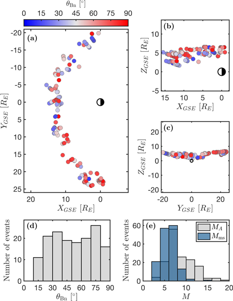
Figure 1. The MMS shock crossings used in this study. (a)–(c) Position of the shock crossing events in GSE in relation to the Earth. The color of the dots indicates the local shock angle. (d) Shock angle distribution. (e) Alfvén and magnetosonic Mach number distribution. One shock crossing with MA ∼ 55 is not shown.
Download figure:
Standard image High-resolution image2.2. Shock Parameters
In order to determine the Mach numbers and shock angle of the bow shock for all events we need to determine the local bow-shock normal vector  for each event. It is in principle possible to determine
  from local measurements of the plasma (e.g., Abraham-Shrauner 1972). However, this can be deceptive when energetic ions are present since the upstream plasma may have large upstream
B
fluctuations that make a local determination of
from local measurements of the plasma (e.g., Abraham-Shrauner 1972). However, this can be deceptive when energetic ions are present since the upstream plasma may have large upstream
B
fluctuations that make a local determination of  and θBn highly inaccurate (e.g., Battarbee et al. 2020). Obtaining
  from timing analysis (Schwartz 1998) is not possible because of the relatively small size of the spacecraft tetrahedron formation, which is ∼20 km in most of the cases studied here. Instead we determine the local bow-shock normal by using the bow-shock model by Farris et al. (1991). We fit the bow-shock model through the position of MMS at the time of the event and obtain
  from this fitted model (Schwartz 1998). This method is possible since all MMS events are in direct contact with the bow shock and the shock parameters we obtain are the average upstream conditions and not local parameters that are sensitive to upstream fluctuations and small-scale structures within the shock. When we have obtained
  , we can calculate the shock-normal angle θBn between the model shock normal and the solar-wind upstream magnetic field obtained from the OMNI database. Another parameter of interest is how far out on the flank of the bow shock MMS is positioned. We define the angle ϕ as the angle between the MMS position and the Sun–Earth line seen from the center of the Earth at the time of the event. Then ϕ = 0 at the subsolar point of the bow shock and large values of ϕ means that MMS is on either the dawn- or dusk-side flank.
We also calculate the Mach number of the shock from the solar-wind parameters provided by OMNI. We calculate both the Alfvén Mach, MA , and the fast magnetosonic Mach, Mms, numbers in the shock frame assuming a zero shock speed relative to the spacecraft. The Alfvén Mach number of the shock is

where
V
u
is the upstream flow velocity, vA
is the upstream Alfvén speed, and θVn
is the angle between  and
V
u
. We also calculate the fast magnetosonic Mach number
and
V
u
. We also calculate the fast magnetosonic Mach number

where the vms(θ) is the fast magnetosonic speed for a propagation angle θ to
B
. We assume that the upstream electron temperature is the same as the ion temperature Ti
so that the sound speed  , where mi
is the proton mass and kB
is the Boltzmann constant.
, where mi
is the proton mass and kB
is the Boltzmann constant.
The shock angle and Mach number distributions of the MMS shock crossings are shown in Figures 1(d)–(e). Compared to the typical solar wind, quasiparallel shock geometries are somewhat overrepresented, likely due to selection bias in the SITL reports. The Mach numbers have rather typical solar-wind values with MA ∼ 5–15 and Mms ∼ 3–8, although with some limitations on high Mach number by the selection condition that FPI-DIS covers energies greater than 20 times the solar-wind energy. This data set has a good coverage of quasiparallel and quasiperpendicular shock regions as well as low to high Mach numbers.
2.3. Acceleration Efficiency
Next, we quantify the presence of high-energy ions at the shock in order to compare this value to the derived shock parameters. We adopt the same definition as Caprioli & Spitkovsky (2014a) of ion acceleration efficiency ε(E0) to be the fraction of energy density of ions with energy Ei > E0 to the total ion energy density, measured in the downstream. We express this as
where Ui (Ei > E0) is the ion energy density above the energy E0 and the brackets indicate time averaging over a downstream interval. In this definition of ion acceleration efficiency, we assume that most available energy in the shock goes to the ion population, either by heating or acceleration. The benefit of this definition is that it naturally adopts a value between 0 and 1, and is less sensitive to uncertainties in upstream plasma measurements than definitions based on energy flux as used by e.g., Ellison et al. (1990). This makes the definition of ε based on energy density well suited for our study with many shock crossings and somewhat uncertain upstream conditions. The ion energy density can be expressed as
where fi
(Ei
) is the spherical mean of the ion phase-space density as a function of energy. Like Caprioli & Spitkovsky (2014a) we investigate ion acceleration efficiency above an energy E0 = 10Esw, where  is the solar-wind bulk energy and Vsw the solar-wind bulk speed. We refer to these ions as energetic. We will however also be investigating ion acceleration above 5Esw, which we refer to as suprathermal (Caprioli et al. 2015). To be able to calculate the ion acceleration efficiency we need to know at what parts of the time intervals MMS is in the downstream. We manually select the downstream times for all events. We set the downstream intervals from where the ion distribution is significantly thermalized and where the plasma density is increased. The time averaging in ε is then done in these intervals.
To truly represent acceleration efficiency, Ui should be measured in the downstream frame of reference. Therefore, we calculate fi (Ei ) in the local downstream plasma frame. This is done by calculating the average phase-space densities in spherical shells centered on the plasma flow velocity. This allows for a direct comparison of acceleration efficiency at shock crossings with different downstream flow speeds.
Next, we look closer at three shock crossings by MMS from the data set. The events are shown in Figure 2. The manually determined downstream intervals are marked in gray. The first event shown in Figures 2(a)–(b) shows a quasiperpendicular shock. As typical for quasiperpendicular shocks, the transition from upstream to downstream is sharp. As can be seen, there are practically no ions with energy E > 10Esw and therefore the ion acceleration efficiency is close to zero. Figures 2(c)–(d) shows an encounter with the quasiparallel bow shock close to the subsolar point. Here, the shock transition is much patchier and more extended. During the time interval, MMS observes three Short Large Amplitude Magnetic Structures (SLAMS) (Schwartz & Burgess 1991) seen as sharp increases in B in the upstream. The last SLAMS appears to be merging with the shock proper and the plasma transitions to downstream at this point. As we can see in Figure 2(d), there is a large density of energetic ions at this time and the acceleration efficiency is relatively high with 6% of the ion energy density being contained in energetic ions. The last shock crossing in Figures 2(e)–(f) also shows a quasiparallel shock crossing. In this event, MMS crosses the bow shock quite far out on the flank of the dawn side of the bow shock. Compared to the previous event, the Mach number MA is also lower. Here, ions are clearly accelerated at the shock, but the energy of the ions rarely goes above 10Esw, see Figure 2(f). Therefore, the acceleration efficiency is rather low at 0.1%. As we will see below, these events illustrate trends of ion acceleration in the statistics of all analyzed events.

Figure 2. Example of bow-shock crossings by MMS. (a–b) Quasiperpendicular shock. (c–d) Quasiparallel shock. (e–f) Quasiparallel shock on the bow-shock flank. The time intervals marked in gray show the selected downstream interval for each event. Upper panels: magnetic field magnitude time series; lower panels: omni-directional ion energy spectrogram in the spacecraft frame. The dashed lines in the spectrograms show E = 10Esw.
Download figure:
Standard image High-resolution imageThe Earth's bow shock is relatively small in astrophysical settings and has a curved shape. This means that, unless the IMF is perfectly aligned with the solar wind, a field line will only be connected to the bow shock for a limited time. Therefore, we can say that the field lines connected to the bow shock have a limited lifetime, even during stable upstream conditions. Ions that are injected and accelerated at the bow shock will eventually be convected away by the solar wind and therefore only have a limited amount of time to gain energy. We therefore try to estimate how long a field line has been connected to the bow shock when the MMS measurements are made and we call this the connection time Tc
. Scholer et al. (1980) found that energetic ion events upstream of the shock are more probable for high Tc
. Under most circumstances, a field line first connects to the bow shock at the tangent point where θBn = 90°. The field line then traverses the bow shock with decreasing θBn. To calculate Tc
, we first use the same bow-shock model (Farris et al. 1991) we used to determine  to estimate the global shape of the bow shock. We then calculate the position of the tangent plane where the field lines connect to the bow shock where θBn = 90°. We then get Tc
from the distance between the spacecraft and the tangent plane in the direction of the solar wind. We illustrate this procedure in Figure 3, which depicts the bow shock seen from the Sun in the event shown in Figure 2(c)–(d). This method assumes a steady solar wind and we therefore only consider Tc
< 600 s as this was the time we require the OMNI data to be steady, described above. The maximum achievable energy in DSA is expected to increase with Tc
(Axford 1981; Caprioli & Spitkovsky 2014b). Here, we have no information about the maximum energy due to limited energy coverage (<28 keV). We instead use Tc
to investigate the evolution of ion injection into DSA.
to estimate the global shape of the bow shock. We then calculate the position of the tangent plane where the field lines connect to the bow shock where θBn = 90°. We then get Tc
from the distance between the spacecraft and the tangent plane in the direction of the solar wind. We illustrate this procedure in Figure 3, which depicts the bow shock seen from the Sun in the event shown in Figure 2(c)–(d). This method assumes a steady solar wind and we therefore only consider Tc
< 600 s as this was the time we require the OMNI data to be steady, described above. The maximum achievable energy in DSA is expected to increase with Tc
(Axford 1981; Caprioli & Spitkovsky 2014b). Here, we have no information about the maximum energy due to limited energy coverage (<28 keV). We instead use Tc
to investigate the evolution of ion injection into DSA.

Figure 3. Earth's bow shock as seen from the Sun in GSE coordinates for the time 2018 January 29, 03:38 UTC. The upstream magnetic field for this shock crossing is [2.7, 1.9, −0.3] nT and the speed 340 km s−1. (a) The shock angle on the surface of the shock. The position of MMS at this time is shown as a black circle and the tangent line where θBn = 90° is shown by a red line. (b) The time a field line has been connected to the bow shock. The path the field line has taken from the tangent line to the spacecraft position is shown in purple. In this case Tc = 350 s at the MMS position.
Download figure:
Standard image High-resolution imageNow, we look at all 154 selected shock crossings by MMS. Figure 4(a) shows the average phase-space density as a function of energy normalized to Esw for all shock crossings averaged over the downstream time intervals and represented in the local downstream frame. We can see that downstream of the quasiperpendicular bow shock (shown in red colors), the ion distribution is heated and is nearly Maxwellian. There is also a clear bump in the distribution at 2–4Esw. This is the result of ions being reflected at the shock and completing one gyration before going downstream, gaining energy in the process (Paschmann et al. 1980). Downstream of the quasiparallel shock (shown in blue colors), the ions are also heated but retain more of the solar-wind core at Esw. A high-energy tail extending beyond 10Esw is also present downstream of the quasiparallel shock. Next, we use these distributions to quantify the acceleration efficiency at the bow shock.

Figure 4. MMS ion observations downstream of the bow shock. (a) Downstream average phase-space density in the local plasma frame as a function of energy normalized to the solar-wind kinetic ram energy for all 154 events. The color of each curve indicates the shock-normal angle. (b) Ion acceleration efficiency as a function of shock angle θBn for all events. The Alfvén Mach number for each event is indicated with color. θBn = 45° is marked with a dashed line.
Download figure:
Standard image High-resolution imageFigure 4(b) shows a scatter plot of ε(10Esw
), calculated from the distribution functions in Figure 4(a) as a function of θBn. A clear trend is that the acceleration efficiency is close to zero for θBn ≳ 50° in good agreement with (Caprioli & Spitkovsky 2014a). For shocks with θBn≲50° the acceleration efficiency is significantly higher, up to ∼15 %. However, there is a large spread in ε for quasiparallel shocks. The color in Figure 4(b) indicates the Alfvén Mach number. There seems to be a trend of lower ε when MA
is low. This will be investigated further below. Another explanation for the large variations might be the dynamic and turbulent nature of quasiparallel shock waves and the fact that MMS measurements represent a snapshot at one point of the shock. There is also a slight trend for lower ε for θBn < 20°. However, due to the  probability for θBn
, there are few events in this range, making this result uncertain. Overall the acceleration efficiency agrees with simulation results by Caprioli & Spitkovsky (2014a).
probability for θBn
, there are few events in this range, making this result uncertain. Overall the acceleration efficiency agrees with simulation results by Caprioli & Spitkovsky (2014a).
We can clearly see in Figure 4 that ion acceleration efficiency has a strong dependence on the shock angle. Now, we further investigate how ε depends on other shock parameters. The clearest trends are found in the Mach numbers in Figures 5(a)–(b). It is clear that ε is significantly lower for lower Mach numbers MA
< 7 and Mms < 5. Especially for Mms where θBn < 45°, the positive trend to ε seems to continue for the entire parameter range captured here. One clear trend is that ion acceleration is on average much more efficient close to the subsolar point than on the flanks of the bow shock, see Figure 5(c). This result is somewhat unexpected since, although the Mach numbers depend on ϕ, this dependence is too weak to explain the difference in ion acceleration between subsolar and flank bow shock. To further examine this, we study the ε dependence on connection time Tc
normalized to the inverse ion gyrofrequency ωci
in Figure 5(d). We see that Tc
is strongly correlated with θBn. In the quasiparallel regime, however, we see that an increasing connection time first leads to a somewhat higher acceleration efficiency, but that after  there is a decrease in ε. Perhaps surprisingly, we find no correlation between Tc
and ϕ. This is because field lines do not have to pass by the nose of the bow shock but can be connected to flanks of the bow shock all the time.
there is a decrease in ε. Perhaps surprisingly, we find no correlation between Tc
and ϕ. This is because field lines do not have to pass by the nose of the bow shock but can be connected to flanks of the bow shock all the time.
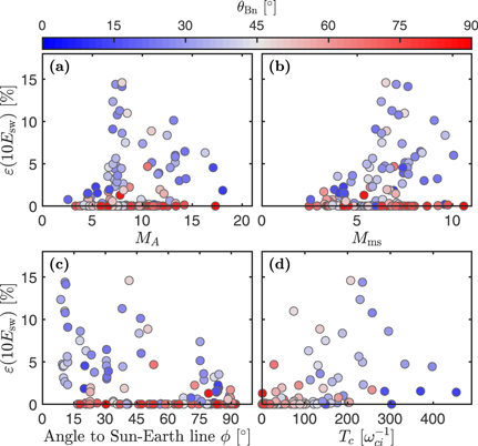
Figure 5. Acceleration efficiency as a function of different parameters. The data points are colored after θBn. Acceleration efficiency as a function of (a) Alfvén Mach number, (b) magnetosonic Mach number, (c) angle to Sun–Earth line, and (d) the field-line connection time normalized to the solar-wind cyclotron period. In (d), only shock crossings where Tc < 600 s are included.
Download figure:
Standard image High-resolution image3. Global Simulations of Ion Acceleration
3.1. Simulation
In order to test and validate the results from the MMS statistics, we compare the observations to a two-dimensional, hybrid-kinetic Vlasiator simulation of Earth's bow shock. Vlasiator (von Alfthan et al. 2014; Palmroth et al. 2018) is a global hybrid-Vlasov model where ions are described as distribution functions and electrons as a cold massless charge-neutralizing fluid. The simulation solves the Vlasov equation coupled with Maxwell's equations to propagate the plasma. The electric field is closed by Ohm's law E = − V i × B + j × B /qe n, where j is the current density, n is the number density, and qe is the elementary charge. The main benefit to a Vlasov scheme is that it uses noise-free distribution functions directly instead of relying on integrating potentially noisy particles like in particle-in-cell simulations.
The simulation used in this study simulates near-Earth space in the meridional plane, ignoring dipole tilt. The simulation plane, which corresponds to the X–Z plane in GSE coordinates, is different from the MMS orbit, which is mainly in the X–Y plane. However, in the context of the bow shock, this simulation setup corresponds to a Parker spiral like setup (Turc et al. 2020). The solar wind in the simulation consists of a purely proton plasma and has a flow speed of 750 km s−1 in the −X direction with a plasma density of 1 cm−3. The IMF is in the simulation plane at  and is therefore southward and forms a 45° angle to the Sun–Earth line. This means that we model the quasiperpendicular and quasiparallel bow shock at the same time. The solar-wind Mach numbers are therefore MA
= 6.9, Mms = 5.9, and ion beta βi
= 0.7. We note that the solar wind is faster than the typical solar wind, but the dimensionless parameters like Mach numbers and ion beta are typical for the solar wind. The extent of the simulation box is X ∈ [ − 48, 64]RE
and Z ∈ [ − 60, 40]RE
with a spatial resolution of 300 km. The 3D velocity space extends ±4000 km s−1 in each direction with a resolution of 30 km s−1. Vlasiator uses a sparse velocity grid in order to save on computational resources. This means that the simulation is only storing the distribution function where f exceeds some value
and is therefore southward and forms a 45° angle to the Sun–Earth line. This means that we model the quasiperpendicular and quasiparallel bow shock at the same time. The solar-wind Mach numbers are therefore MA
= 6.9, Mms = 5.9, and ion beta βi
= 0.7. We note that the solar wind is faster than the typical solar wind, but the dimensionless parameters like Mach numbers and ion beta are typical for the solar wind. The extent of the simulation box is X ∈ [ − 48, 64]RE
and Z ∈ [ − 60, 40]RE
with a spatial resolution of 300 km. The 3D velocity space extends ±4000 km s−1 in each direction with a resolution of 30 km s−1. Vlasiator uses a sparse velocity grid in order to save on computational resources. This means that the simulation is only storing the distribution function where f exceeds some value  (Palmroth et al. 2018). In this case,
  s3 m−6.
Figure 6(a) shows the plasma density in the simulation after a simulation time of 1361 s ( ). We can see the bow shock as a sharp increase in density. The quasiparallel part of the shock at Z < 0 is characterized by large fluctuations in density and magnetic field. The approximate position of the magnetopause is marked and we see a number of flux transfer events formed. One of the flux transfer events has launched a "bow wave" (Pfau-Kempf et al. 2016) toward the bow shock, which slightly distorts the shape of the bow shock. Normally in the simulation, the full 3D ion velocity distribution function is only saved in a few cells each time step. However, here we use data from a time that can be used to restart the simulation. For this time step, the ion distribution function is saved in all simulation cells, allowing for detailed analysis of ion acceleration at the bow shock.

Figure 6. Part of the simulation box at t = 1361 s. (a) Plasma density. The fitted bow-shock model is shown in purple and the approximate magnetopause location is shown in red. (b) Ion energy density of ions with energies above 5Esw. The contour of where n = 2nsw is shown in black. Magnetic field lines in gray are shown in both (a) and (b). (c) Ion acceleration efficiency measured downstream of the shock within 0.5RE of the model bow shock as a function of Z.
Download figure:
Standard image High-resolution imageThe Vlasiator simulation used here trades high spatial resolution for correctly modeling the global processes at the bow shock. The grid cell size in this simulation is 300 km while the upstream ion inertial length is ∼230 km. The thermal gyroradius of a solar-wind ion is ∼190 km and the gyroradius of a specularly reflected ion is on the order of 1000 km. This suggests that not all ion-kinetic physics can be expected to be fully resolved at the bow shock. Despite this, Pfau-Kempf et al. (2018) showed that even when not resolving the ion inertial length, the Vlasiator model is able to correctly model many kinetic effects such as ion reflection and upstream waves in an oblique 1D shock. In addition to this, the main strength of Vlasiator in this study is that it is a noise-free kinetic model while maintaining realistic separation of kinetic and global scales, which allows for direct comparison with observations from the Earth's bow shock.
3.2. Ion Acceleration in Vlasiator
In order to quantify ion acceleration in the simulation we need to estimate where in the simulation the bow shock is located. While assuming a bow-shock shape of a conic section (Schwartz 1998) is often the most accurate when working with spacecraft data, the bow shock in the simulation is distorted due to feedback from kinetic effects and its shape is not well described as a conic section or polynomial. The bow-shock model we are using here for estimating its position is constructed from contour points where the plasma density has a value of 2nsw. This value is used as an approximation to when the plasma transitions from upstream to downstream since the compression ratio at all points of the shock is expected to be greater than two (Battarbee et al. 2020). The model bow-shock shape is then constructed by fitting a smooth curve to these contour points. The estimated bow-shock shape is shown as a magenta line in Figure 6(a) and the contour points used to make the fit in Figure 6(b). Important parameters such as MA and θBn are then calculated everywhere using the normal vector obtained from the model bow-shock curve. We emphasize that this postprocessing does not affect the physics of the simulation.
Figure 6(b) shows the energy density for ions with energy above 5Esw (suprathermal ions) in a region close to and upstream of the estimated bow-shock position. We show the energy density above 5Esw here instead of the 10Esw that we used for the spacecraft observations due to the sparse velocity grid of Vlasiator, which we shall see below leads to the distribution function rolling off at around 10Esw. This is a limitation in the Vlasov scheme of Vlasiator when studying high-energy particles. To get around this limitation we instead quantify the early stage of ion acceleration using 5Esw as a lower energy limit and compare this to the observations with a similar energy limit.
We can see several interesting features in the concentration of suprathermal ions in Figure 6(b). First, it is clear that the quasiperpendicular bow shock produces practically no suprathermal ions and these ions are only found in the quasiparallel region. We can see the presence of a field-aligned beam upstream of the bow shock originating from the shock where θBn ∼ 45° (Kempf et al. 2015). There seems to be no increase of suprathermal ions just downstream of where the field-aligned beam connects to the bow shock. Further out on the flank on the quasiparallel side the suprathermal ions are found close to the bow shock and extend both in the upstream and downstream. The extent of the suprathermal ions on the upstream side seems to increase further out on the flank. As the position on the flank translates to the time a field line has been connected, this indicates a DSA-like acceleration of the ions (Jones & Ellison 1991). The energy density of these ions is also highly structured in the upstream. The details of how the upstream suprathermal ion population evolves and how it is modulated by fluctuations like SLAMS-like structures in Vlasiator are left for a future study.
Next, we investigate the downstream ion distributions to quantify ion acceleration in the simulation. Therefore, we divide all simulation points in bins based on their angle to the Sun–Earth line. We use 256 equally-spaced bins in ϕ between −100° and 80◦, where negative angles correspond to Z < 0. To better compare with the spacecraft observations which were made in direct contact with the shock, we only use simulation cells that are within a distance of 0.25RE ≈ 1600 km to our bow-shock estimate. Lastly, we put a constraint for n>2nsw in order to only use cells that we estimate to be downstream of the shock. The resulting average ε measured in the local downstream plasma frame is shown in Figure 6(c) along the Z position of the bow shock. It is clear from the figure that ε is higher on the quasiparallel side that there is a large spread in ε and that ε seems to decrease on the flank of the bow shock, all consistent with the observations.
The average distributions for each ϕ bin are shown in Figure 7(a). These downstream distributions show similarities to those observed by MMS in Figure 4(a) in that the high-energy tail extending further for quasiparallel shock geometries. However, as can be seen in Figure 7(a), the ion distributions appear to roll off at ∼10Esw. This is due to the sparse velocity grid used in Vlasiator.
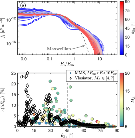
Figure 7. Ion distributions and acceleration efficiency in Vlasiator. (a) Average downstream distributions in the plasma frame of reference within 0.25RE from the bow shock colored after θBn. The gray dashed line shows a Maxwellian distribution from the downstream conditions given by the Rankine–Hugoniot conditions at Z = 30RE and θBn = 80°. (b) Acceleration efficiency of ions above 5Esw. The MMS measurements of the acceleration efficiency of ions with 5Esw < E < 10Esw are shown as filled circles colored after MA and the Vlasiator data are shown as black diamonds.
Download figure:
Standard image High-resolution image
One difference between the ion distributions observed by MMS and in Vlasiator is found in quasiperpendicular shock geometries. The simulation results do show a bump in the ion distributions at 2–4Esw due to ion reflection when θBn > 45°. It is, however, less clear than in the MMS observations. One explanation could be that the Mach number in the simulation is lower than most events in the MMS data set and that ion reflection is less efficient at lower Mach numbers. Another reason for the difference could be that Vlasiator does not correctly model the ion reflection at the quasiperpendicular shock, possibly due to the limited spatial resolution and that the electron pressure gradient term is omitted in Ohm's law. However, we estimate the electron pressure gradient term would contribute at most 10% of the shock-normal electric field at the quasiperpendicular shock. We also observe clear evidence of near-specular ion reflection at this part of the shock and that ∼10% of the solar-wind ions are reflected (c.f. Leroy et al. 1982). We shall further investigate ion distributions at the quasiperpendicular shock in a future study, as well as effects of spatial resolution.
The ion acceleration efficiency above 5Esw as a function of θBn is shown in Figure 7(b). The simulation results are shown on top of the MMS observations. To better compare the measurements to the simulation, we show the acceleration efficiency measured by MMS using only the part of the distribution with 5Esw < E < 10Esw. Like in Figure 4(b), we see that ion acceleration for this energy limit is much higher on the quasiparallel parts of the bow shock. The Vlasiator results show a qualitative match with the low Mach number shock crossings by MMS. Vlasiator also shows a large spread in acceleration efficiency in the quasiparallel part, further highlighting the dynamic nature of ion acceleration in this region of the bow shock. The simulation seems to show that ion acceleration starts to become efficient below θBn ≲ 30° rather than θBn ≲ 50° for the MMS observations. We also find no decrease in the acceleration efficiency for θBn < 20°, suggesting that the simulation does not fully capture the θBn-dependence on the ion acceleration efficiency. We note that the observed θBn-dependence is more similar to that found in simulations by Caprioli & Spitkovsky (2014a) than what we find in the Vlasiator simulation. Except for this, ion acceleration efficiency in the Vlasiator simulation shows good quantitative agreement with observations of the bow shock by MMS.
Even though we are using only one time step of the simulation, the general curved shape of the bow shock allows us to investigate the time evolution of the suprathermal ions at the shock. Because of the two-dimensional simulation setup, determining the time a field line has been connected to the bow shock is somewhat simplified from a true 3D case. To determine the connection time Tc , we find the field line, which is connected to the tangent point where θBn = 90° and determine Tc from the solar-wind speed and the distance along X between this line and the model bow shock. We estimate that the connection time is 120 s (250ωci ) at the subsolar point and 370 s (770ωci ) on the outermost flank in Figure 6. The bow-shock shape in the simulation stabilizes at a time before 800 s while the time step here is 1361 s, so the travel time estimates are not affected by simulation initialization and the large-scale bow shock shape changes.
It is clear from Figure 6(c) that the ion acceleration at the shock is less efficient on the far quasiparallel flank of the bow shock, similar to the MMS observations. In a 2D setup like this, the connection time Tc
increases with Sun–Earth angle ϕ on the −Z flank. This would thus lead to the interpretation that, at very large values of Tc
, the acceleration efficiency would decrease. Terasawa (1979) showed that in a curved shock, particle injection changes over connection time Tc
as a function of local acceleration efficiency (in their model, magnetic compression and effective shock velocity). Like them, we also see a decrease in magnetic compression ratio at the quasiparallel flank, explaining how large values of Tc
can in fact be connected with low-acceleration efficiency  , and how Tc
in itself is insufficient to estimate particle energization. Similarly, in the MMS observations, we see acceleration efficiency initially increase with Tc
, then decreasing after
, and how Tc
in itself is insufficient to estimate particle energization. Similarly, in the MMS observations, we see acceleration efficiency initially increase with Tc
, then decreasing after  (see Figure 5(d)). This decrease happens despite the connection time having no correlation with the angle ϕ due to the 3D nature of the bow shock. These results, being in agreement, suggest that the relevant acceleration timescale to energies 5–10Esw is much less than the field-line connection timescale.
4. Discussion
A previous study of high-energy ions performed far upstream of the Earth's bow shock by Kronberg et al. (2011) found that at least some of the events were from a magnetospheric origin. In this study, we are interested in ions that are accelerated from the solar-wind population at the shock and not ions escaping from the magnetosphere. Fuselier et al. (1991) found that a majority of energetic ion events (10–17 keV) in the magnetosheath show no O+ signature and therefore originate from the shock. Only very infrequently did they observe a magnetospheric O+ when the measurement was performed far away from the magnetopause. The Vlasiator simulation produces a high-energy ion population in the magnetosphere but it is clear that the suprathermal ions are observed close to the shock. Therefore, we conclude that the energetic ions in the simulation and observed by MMS are accelerated locally at the shock.
In contrast with those previous shock acceleration studies that have employed local hybrid-kinetic simulations of planar shocks, our study uses a global simulation capable of evaluating both quasiparallel and quasiperpendicular sections of the shock. Our shock reacts to foreshock disturbances and magnetosheath bow waves in a realistic manner and allows for assessing DSA efficiency as a function of field-line age Tc as well as providing ample parameter space for assessing shock energization in relation to nose angle ϕ and shock-normal angle θBn. Assessing multiple regions along the bow shock within the same simulation allows for interplay between SDA-energized particles originating in the quasiperpendicular region and the efficient DSA process in the quasiparallel region.
5. Conclusions
In this work, we study a collection of 154 shock crossings by the MMS spacecraft and compare the results to a global hybrid-Vlasov Vlasiator simulation in order to study the properties of ion acceleration at the Earth's bow shock.
We select 154 shock crossings by the MMS spacecraft. We use solar-wind measurements by upstream spacecraft through the OMNI database and verify them with MMS. High-energy ions are present in many of the studied shock crossings. We conclude that these ions are accelerated locally and magnetospheric sources are unlikely. The acceleration efficiency, defined as the fraction of energy density in ions with more than 10 times the solar-wind energy measured in the downstream, is significantly higher at quasiparallel shocks with values up to 15% of the energy going to accelerate ions above 10Esw. When θBn > 50°, practically no energetic ions are observed, indicating a very low acceleration efficiency. We find that ion acceleration efficiency is significantly lower for shocks with MA
< 7 or Mms < 5 with a trend of increased ion acceleration at higher magnetosonic Mach numbers. A clear trend in the data is a decreased ion acceleration efficiency at both flanks of the bow shock. This appears to be partly correlated with lower Mach numbers on the flanks, but we also investigated the total time a field line had been connected to the bow shock. The observations here seem to suggest that a higher connection time leads to an increased acceleration efficiency. This trend does not appear to extend past  . Most of these results are quantitatively in good agreement with 2D simulations of the planar shocks by Caprioli & Spitkovsky (2014a).
To supplement our MMS observations, we perform a statistical analysis of ion acceleration efficiency using a global hybrid-Vlasov Vlasiator simulation of the Earth's bow shock. Our simulation shows both quantitative and qualitative agreement with the MMS observations. We again find that ion acceleration efficiency is low in the quasiperpendicular region and higher in the quasiparallel region. The highest acceleration efficiency in Vlasiator is found where θBn ≲ 30° rather than 50° found in the MMS observations. Within the quasiparallel region, ion acceleration efficiency ε is patchy and can vary between <1% and over 10% before again diminishing when reaching the far flank.
Although the age Tc of field lines connected to the bow shock is shown to not be a strong controller of observed acceleration efficiency, our simulations show that this is not solely due to field lines potentially traversing along the flanks never reaching the quasiparallel nose region. Instead, even field lines which have convected across the whole shock can have low instantaneous acceleration efficiency due to both dynamic perturbation of the shock front and previously accelerated ions convecting and diffusing away from the shock front. Acceleration efficiency ε appears to be greatest in the quasiparallel region closest to the shock nose where SDA-accelerated ions originating from the oblique θBn ∼ 45° shock region can possibly act as seed particles for efficient DSA. In this region, it appears that the bow shock undergoes a burst of suprathermal ion acceleration to later relax to a steadier state on the flank consistent with previous simulation results (Caprioli & Spitkovsky 2014a) and possibly our MMS observations presented here.
Acceleration of ions at the terrestrial bow shock is thus shown to be a multifaceted process, involving both local and global interactions of ions and shock structures. Our statistical analysis shows clear trends and dependencies on, e.g., Mms and θBn, but also highlights significant variation due to unpredictable plasma disturbances. Thus, a combination of observational and simulational statistical studies is shown to be a fruitful approach for investigating energetic particle processes at plasma shocks.
This research was made possible with the data and efforts of the people of the Magnetospheric Multiscale mission. The data are available through the MMS Science Data Center 8 and the CDA Web. 9 The OMNI data were obtained from the GSFC/SPDF OMNIWeb interface at https://omniweb.gsfc.nasa.gov. We thank the anonymous reviewer for comments that greatly helped to improve the paper. We acknowledge the European Research Council for Starting grant 200141-QuESpace, with which Vlasiator was developed, and the Consolidator grant 682068-PRESTISSIMO awarded to further develop Vlasiator and use it for scientific investigations. The CSC-IT Center for Science in Finland is acknowledged for the Sisu supercomputer pilot usage and Grand Challenge award leading to the results presented here. We thank Rami Vainio for assistance in performing the simulation. The work is supported by Academy of Finland grants: the Finnish Centre of Excellence in Research of Sustainable Space grant number 312351, grant number 267186, and the work of LT through grant number 322544. We also acknowledge support from Swedish National Space Board Contracts 139/12 and 97/13. The work was supported by the International Space Science Institutes (ISSI) International Teams program 454.