


Abstract
The radio sky at frequencies below ∼10 MHz is still largely unknown; this remains the last unexplored part of the electromagnetic spectrum in astronomy. The upcoming space experiments aiming at such low frequencies (ultralong wavelengths or ultralow frequencies) would benefit from reasonable expectations of the sky brightness distribution at relevant frequencies. In this work, we develop a radio sky model that is valid down to ∼1 MHz. In addition to discrete H ii objects, we take into account the free–free absorption by thermal electrons in the Milky Way's warm ionized medium. This absorption effect becomes obvious at ≲10 MHz, and could make the global radio spectrum turn over at ∼3 MHz. Our sky map shows unique features at the ultralong wavelengths, including a darker Galactic plane in contrast to the sky at higher frequencies, and huge shadows of the spiral arms on the sky map. It will be a useful guide for designing future ultralong-wavelength observations. Our Ultralong-wavelength Sky Model with Absorption (ULSA) model can be downloaded at doi:10.5281/zenodo.4454153.
Export citation and abstract BibTeX RIS
1. Introduction
The radio sky has been surveyed from ∼10 MHz up to ∼1 THz. Based on data of surveys at the relevant frequencies, full-sky maps have been produced at 408 MHz (Haslam et al. 1982; Remazeilles et al. 2015), 1.42 GHz (Reich 1982; Reich & Reich 1986; Reich et al. 2001), and a number of higher frequencies from 22.8 GHz to 857 GHz by the Wilkinson Microwave Anisotropy Probe and Planck satellite (see Hinshaw et al. 2009; Planck Collaboration et al. 2016a). In addition, there are surveys that cover a large portion but not the full sky. In order to produce sky maps at frequencies in which the full sky has not been surveyed, a number of sky models have been developed, based essentially on interpolation or extrapolation of the available data, and statistical modeling of the sky intensity distribution. Over much of the radio wave band, the sky intensity has a nearly power-law spectrum, making interpolation/extrapolation relatively simple and accurate. These models include the Global Sky Model (de Oliveira-Costa et al. 2008), its improvements (Danny 2016; Zheng et al. 2017; Sathyanarayana Rao et al. 2017; Kim et al. 2018), and the Self-consistent Sky Model (Huang et al. 2019). They are very useful in the design of new instruments, the study of observation strategies, and the testing of foreground removal/mitigation methods (e.g., Shaw et al. 2014; Zuo et al. 2019).
However, extrapolation becomes trickier at frequencies ≲10 MHz, where the absorption of the interstellar medium (ISM) becomes significant, and at the same time there is a dearth of observation data. Observations below 10 MHz are severely hampered by the absorption and distortions of the ionosphere (Jester & Falcke 2009). To date, there have been only a few ground-based observations, performed during the ∼1950s–1960s (George et al. 2015; Cane & Whitham 1977), and a few space-based low-resolution observations, performed during the ∼1960s–1970s (Alexander et al. 1969; Brown 1973; Alexander & Novaco 1974; Alexander et al. 1975; Cane 1979). Below we shall call this wave band the ultralong-wavelength or ultralow-frequency band, though these are not the names used by radio engineers. The ultralong-wavelength sky is still a largely unexplored regime in astronomical observations. To open this new window in the electromagnetic spectrum, a number of space missions, e.g., the lunar-orbit array for Discovering the Sky at the Longest Wavelength (Chen et al. 2019), and the lunar-surface-based FARSIDE (Burns et al. 2019), have been proposed, with the aim of obtaining high-resolution 5 full-sky maps at ultralong wavelengths.
However, to design such low-frequency experiments and observe the sky at this largely unexplored part of the electromagnetic spectrum, one needs a reasonable estimate of the sky brightness at these frequencies, and a fair expectation of the structures, so that the required system gain and dynamic range can be derived. More importantly, at present or in the near future, a lunar-orbit or lunar-surface-based array necessarily has a limited number of antenna elements (though the orbital precession could improve the uvw coverage at the expense of longer observation time), and the antennas are all-sky sensitive; these make the imaging process quite challenging, especially when the sky brightness itself varies dramatically with frequency and direction, as we will show below. It is therefore crucial to have a reasonable full-sky model for these unexplored frequencies, which could serve as a starting point for the deconvolution process, for both end-to-end simulations in designing such experiments and the upcoming real observations.
At ≲10 MHz, the existing sky models based on extrapolation are grossly inadequate, because free–free absorption and synchrotron self-absorption (Orlando & Strong 2013; Ghisellini 2013) become very significant. In the Galactic diffuse ISM the former is much more important (Scheuer & Ryle 1953; Shain 1959; Hurley-Walker et al. 2017). Free–free absorption is the inverse process of bremsstrahlung (free–free) radiation, so it is proportional to the square of free-electron density. The absorption level depends not only on the smoothed distribution, but also on the small-scale turbulence.
In as early as the 1960s, it was discovered that the global radio background (the sum of Galactic and extragalactic radiation) spectrum has a downturn at ∼3–5 MHz, by ground-based telescopes (e.g., Ellis & Hamilton 1966), by radio astronomy rockets (e.g., Alexander & Stone 1965), and by space satellites (e.g., Ariel II, Smith 1965; RAE-1, Alexander et al. 1969; IMP-6, Brown 1973; and RAE-2, Novaco & Brown 1978), and free–free absorption is probably the reason for this downturn in the spectrum. However, it is also possible that the intrinsic energy spectrum of the cosmic-ray particles becomes softer at low energy (Strong & Moskalenko 1998). More references about early low-frequency observations can be found in Cane (1979).
For dense electron clumps, such as those in discrete H ii regions, free–free absorption could make these objects opaque even for radio signals at higher frequencies (e.g., Odegard1986; Kassim 1988). This effect can be used to separate the synchrotron emissivity behind and in front of such regions. If there are a sufficient number of such H ii regions with known distance, the 3D distribution of the synchrotron emissivity could be reconstructed. This has been successfully put into practice (see, e.g., Nord et al. 2006; Hindson et al. 2016; Su et al. 2017, 2018; Polderman et al. 2019 and references therein). Since synchrotron radiation is produced by cosmic-ray electrons in a magnetic field, the cosmic-ray electron distribution can be inferred if the magnetic field is known by other means (Polderman et al. 2020). The degeneracy between the cosmic ray and the magnetic field could also be broken by combining with gamma-ray observations (Nord et al. 2006), as the Galactic gamma ray is mainly from collisions between cosmic-ray particles and ISM particles (Nava et al. 2017), and the ISM density profile could be constructed from 21 cm, CO, and dust thermal emission observations (Ackermann et al. 2012).
A sky model for ultralong wavelengths has to take into account free–free absorption so as to give a reasonable prediction for upcoming observations (Reynolds 1990). In this work, we develop an observation-based sky model that is still valid below ∼10 MHz, by including the free–free absorption effect. We start with a description of our methods in Section 2, which incorporate a fitting result for the Galactic synchrotron spectral index, a fitted Galactic synchrotron emissivity, and an adopted electron density distribution that is responsible for the free–free absorption. The main results are given in Section 3, including the model with a constant spectral index, the model with a frequency-dependent spectral index, and the one with a direction-dependent spectral index. Lastly, we summarize our main conclusions in Section 4. A brief description of our software is presented in the Appendix.
2. Methods
Free–free absorption becomes significant at low frequencies. The optical depth can be written as the integration of the absorption coefficient, κν , along the line of sight,

where ne and Te are the electron density and temperature at  , respectively. For constant electron temperature, the following approximation holds (Condon & Ransom 2016):
where the emission measure (EM) is the integration of electron density squared at all scales,

The ISM inside the Milky Way, the circumgalactic medium (CGM), and the intergalactic medium (IGM) can all absorb low-frequency radio waves. We can make some simple estimates to assess absorption on the various astrophysical scales.
Regarding the CGM, van de Voort et al. (2019) have investigated the distribution of hydrogen surrounding Milky Way–size galaxies from high-resolution zoom-in cosmological hydrodynamic simulations with star formation. They presented the column number density of the hydrogen as a function of r in their Figure 2. We adopt a similar radial density profile, and assume that the free-electron density follows the same distribution, with a clumping factor of ∼3 and a CGM electron temperature of ∼105 K. We find τCGM = 0.9, 0.09, and 0.007 for 1, 3, and 10 MHz, respectively. Thus, the CGM is nearly transparent above 1 MHz, but becomes opaque below 1 MHz. If, however, there are some cooler dense clumps in the CGM, the absorption will be stronger.
The EM of the IGM up to a redshift z is

where  is the clumping factor at
  , and
, and ![${{dr}}_{{\rm{p}}}^{\prime} ={cdz}^{\prime} /[(1+z^{\prime} )H(z^{\prime} )]$](https://content.cld.iop.org/journals/0004-637X/914/2/128/1/apjabf55cieqn4.gif) is the proper distance element at
is the proper distance element at  . Also
  is the mean free-electron density at z, with
  cm−3 being the mean hydrogen number density at present. Note that to use the EM as in Equation (2), we add the factor
  to correct for the redshift dependence of the absorption for a given observing frequency at ν. Since κν
∝ ν−2.1 (Condon & Ransom 2016) and
to correct for the redshift dependence of the absorption for a given observing frequency at ν. Since κν
∝ ν−2.1 (Condon & Ransom 2016) and  , we have
  , and hence

We use the tanh model to describe the reionization history for both H i and He i, and He ii, i.e.,

and

Here y(z) = (1 + z)3/2,  ,
,  , and nHe/nH ≈ 0.083. For H i and He i, we assume
  and Δz = 0.5, and for He ii, we adopt
  and Δz = 0.5 (Planck Collaboration et al. 2020). We use the clumping factor model that fits reionization simulations presented in Iliev et al. (2007), but renormalize it to 3.0 at z = 5, i.e.,

The IGM free–free absorption optical depths at frequencies 1, 3, and 10 MHz are shown in Figure 1 as a function of z; they are not large even at 1 MHz.
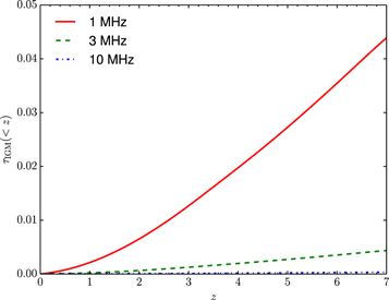
Figure 1. The IGM mean optical depth for ν = 1, 3, and 10 MHz up to redshift z.
Download figure:
Standard image High-resolution imageNext we consider the ISM, which is much denser than the IGM and CGM. The observed sky brightness temperature in the direction given by Galactic coordinates (l,b) is the sum of the Galactic radiation TG(ν, l, b) and the extragalactic background TE(ν),
where sG is the maximum distance to the edge of the Milky Way along any line of sight,  is the 3D radiation emissivity in Galactic-centric cylindrical coordinates (R, Z, ϕ), and τ(ν, s) is the free–free absorption optical depth integrated up to a distance of s. Here we set sG = 50 kpc.
  is the extragalactic radio background, which we assume to be isotropic in the first approximation. With models of an extragalactic radio background
  at ultralong wavelengths, a 3D emissivity (ν, R, Z, ϕ), and a 3D distribution of free electrons in the Milky Way ne, we can derive the sky map at the required frequencies from Equation (10). In the following subsections, we describe the modeling of
  , , and ne.
2.1. The Isotropic Extragalactic Background
The extragalactic background is assumed to be largely isotropic, and a summary of some past results is given in Guzmán et al. (2011). Two methods are commonly used to extract it from the observed sky maps (Kogut et al. 2011; Seiffert et al. 2011). In the first approach the Galactic radiation is described by a plane-parallel model, so the total radiation is

where both  and TG depend only on frequency. In the second approach, the Galactic radiation is derived from a tracer, usually the Galactic [C ii] emission:

where ICII is from the CORE/FIRAS measurements. In practice, all coefficients are fitted from observed radio maps and these two methods give consistent results (Kogut et al. 2011; Dowell & Taylor 2018). However, whether the extracted isotropic background really originates from extragalactic sources is still being debated. Seiffert et al. (2011) extracted a background that is larger than the integrated radio emission of external galaxies (Gervasi et al. 2008). The excess could be from unknown extragalactic source populations, or could be unaccounted-for Galactic foreground (see also Subrahmanyan & Cowsik 2013).
Here we assume that the isotropic background is from extragalactic sources. We adopt the following simple model of isotropic extragalactic background:

This is the fit obtained by the ARCADE-2 balloon experiment, which observed the absolute brightness temperature of the sky between 3 and 90 GHz (Seiffert et al. 2011), minus the cosmic microwave background. This is in good agreement with the fit obtained from the Long Wavelength Array (LWA) (Dowell & Taylor 2018) below 100 MHz. Strictly speaking, "background" is the cumulative radiation from unresolved sources, so it depends on the sensitivity and angular resolution of the telescope. For simplicity we directly use the background fit given by the ARCADE-2 experiment, since in our model we do not specify any particular instrument.
In addition to absorption by the Milky Way, the extragalactic radio background would also be absorbed by the ISM in the host galaxies. Moreover, the spectrum of relativistic electrons could become softer at lower energy, resulting in a softer extragalactic radio background (Protheroe & Biermann 1996). In a recent estimate for the extragalactic radio background, Niţu et al. (2021) found the extragalactic radio background deviates from power law below ∼1 MHz. In Section 3.3 we investigate the case where the extragalactic radio background is not in power-law form.
2.2. Galactic Free–Free Emission
Free–free emission also contributes to the low-frequency sky brightness and should be subtracted from the observed maps for the purpose of assessing Galactic synchrotron radiation. A free–free template could be constructed by using the Hα emission line as a tracer. After correcting the absorption and scattering, the intrinsic Hα flux could be converted into free–free flux (Dickinson et al. 2003; Lian et al. 2020). Moreover, it can be constructed from multifrequency microwave observations. In this work, we use EM and Te maps constructed from Planck multifrequency observations (Planck Collaboration et al. 2016b) 6 to derive the free–free map:
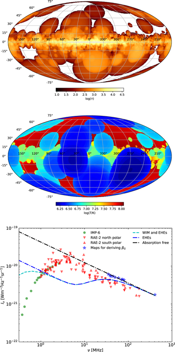
where ν9 is the frequency in units of 109 Hz and T4 is the electron temperature in units of 104 K (Draine 2011). In the top panel of Figure 2, we show the 408 MHz Galactic free–free emission map constructed from the Planck observations. The bottom panel shows the Galactic free–free spectrum. Clearly, most of the free–free emission is from the Galactic plane.

Figure 2. Top: the Galactic free–free emission map at 408 MHz. Bottom: the spectrum of the mean Galactic free–free emission.
Download figure:
Standard image High-resolution imageComparing the above free–free map with observations at 408 MHz (see next subsection), we find that the free–free emission contributes 4% of the mean observed sky brightness. At ∣b∣ > 10°, the free–free fraction decreases to 1%. If we smooth both maps with a resolution of 10°, then the rms contributed by the free–free emission is 15% of the total, while at ∣b∣ > 10° the rms fraction decreases to 6%. This is consistent with Dickinson et al. (2003).
2.3. The Absorption-free Sky Map
We first derive the synchrotron spectral index from the observed sky maps at frequencies where absorption is assumed to be negligible. At low frequencies, there are full-sky maps at 408 MHz (Haslam et al. 1974, 1981, 1982; Remazeilles et al. 2015) and 1.42 GHz (Reich 1982; Reich & Reich 1986; Reich et al. 2001). Here we use the free–free subtracted Haslam 408 MHz map as the base, assuming that in the absence of absorption, the brightness temperature of the Galactic synchrotron radiation follows a power-law form (Platania et al. 1998; Kogut 2012; McKinley et al. 2018),

where ν* = 408 MHz. We determine βG by minimizing
where Ti (νj ) is the observed brightness temperature of the ith pixel in the sky map at frequency νj , and TG,i (ν*) is the Galactic radiation for the ith pixel at ν*. The summation is performed for all available pixels at all observed frequencies of our selected data.
Below several hundred megahertz, there are observed sky maps, each of which covers a part of the sky. In determining the spectral index, in addition to the Haslam 408 MHz map, we use a selection of observations that have large sky coverages: the 45 MHz sky map in combination with two observations (Guzmán et al. 2011), and the 35 MHz,
7
38 MHz, 40 MHz, 50 MHz, 60 MHz, 70 MHz, 74 MHz, and 80 MHz maps observed by the LWA (Dowell et al. 2017). The Guzman 45 MHz map covers 96% of the sky, with resolutions of 4 6 × 24 and 36 × 36 for the southern and northern sky, respectively. It combines two surveys performed by devices of similar characteristics. All of the LWA maps cover a total of about 80% of the sky, with resolutions ranging from 48 × 45 to 21 × 20. As the different maps have different angular resolutions, we smooth all the maps with a beam with FWHM = 5° when deriving the power-law index. For all the maps we subtract the free–free emission given in Section 2.2. Our fiducial model assumes that the spectral index is a constant, but we will also investigate a model with a frequency-dependent spectral index in Section 3.3 and a model with direction dependence in the spectral index in Section 3.4.
Using the above method, we derive a spectral index βG = −2.51 for the Galactic synchrotron radiation. This is actually quite similar to the spectral index of the extragalactic background, βE = −2.58. In Figure 3 we plot the 1 MHz sky map that is extrapolated from the free–free subtracted Haslam 408 MHz map using βG = −2.51 for the Galactic component and βE = −2.58 for the extragalactic component. As this is a simple power-law extrapolation, its structure is the same as that of the Haslam 408 MHz map, except for the different temperature scale. This map could be compared with the absorption-included maps presented later in this paper.
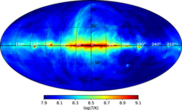
Figure 3. Simple extrapolation of the free–free subtracted Haslam 408 MHz map to 1 MHz without absorption.
Download figure:
Standard image High-resolution image2.4. The Galactic Emissivity Model
We tentatively adopt an axisymmetric form for the Galactic emissivity . In cylindrical coordinates, the emissivity can be written as
Here r1 is a small cutoff radius to avoid singularity at the Galactic center, and we take r1 = 0.1 kpc. The five frequency-independent free parameters—A, R0, α, Z0, and γ—will be obtained by fitting the free–free subtracted Haslam 408 MHz map. The parameter βG is generally a function of frequency and spatial position. Below we take the case of a constant βG as our fiducial model, but also discuss the cases of a frequency-dependent βG and a direction-dependent βG.
Before deriving the emissivity parameters, we mask the Loop I and North Polar Spur (NPS) regions. They are generally believed to be nearby objects (see, e.g., Wolleben 2007), which do not suffer from absorption on the Galaxy scale; hence one should not use these to derive the parameters of the Galactic emission and absorption model. We fit the emissivity parameters from the free–free subtracted Haslam 408 MHz map and the fitted parameters are listed in Table 1.
Table 1. Fitted Galactic Emissivity Model Parameters
| A | 43.10 K kpc−1 |
| R0 | 3.41 kpc |
| α | 0.46 |
| Z0 | 1.12 kpc |
| γ | 1.23 |
Download table as: ASCIITypeset image
2.5. The Galactic Free-electron Distribution
Most free electrons in the ISM are either in the warm ionized medium (WIM), with typical density of ∼0.01–0.1 cm−3 and typical temperature of ∼104 K (Gaensler et al. 2008; de Avillez et al. 2012), or in the hot ionized medium, with typical density of ∼10−3 cm−3 and typical temperature of ∼105–106 K (Ferrière 2001). The free–free absorption is dominated by the WIM. In addition, there are some dense H ii regions with typical density of ∼102 cm−3 and typical temperature of several thousand kelvins (Hindson et al. 2016). They are almost opaque to low-frequency radio radiation, and hence good for separating contributions to the synchrotron radiation from different distances along lines of sight (Su et al. 2017, 2018; Polderman et al. 2019). Moreover, around the dense H ii regions, there could be some extended H ii region envelopes (EHEs), as inferred from observations (Anantharamaiah 1986; Kassim 1989). They have lower densities (∼0.5–10 cm−3) but larger sizes (∼0.05–0.2 kpc) than the classical H ii regions. These could also potentially contribute much to the absorption.
There are a variety of models for the Galactic electron distribution (e.g., Gaensler et al. 2008; Gómez et al. 2001; Taylor & Cordes 1993; Cordes & Lazio 2002, 2003; Yao et al. 2017 (YMW16); Schnitzeler 2012). In the present work, we mainly focus on the general effect of the absorption, so we adopt the NE2001 model (Cordes & Lazio 2002, 2003) for the electron density, which is one of the most well-accepted models. In NE2001, the Galactic free electrons have five components, i.e., smooth components including a thick disk, a thin disk, and five spiral arms; the Galactic center component; the local ISM; a list of known dense clumps; and a list of voids. The dense clumps are mainly H ii regions around massive OB stars or supernova remnants (SNRs). The voids are low-density regions found between the Sun and some pulsars. The smooth components contain lots of free-electron clouds and their volume filling factor is η. The cloud-by-cloud density fluctuations are described by the parameter
where nc is the free-electron density of the cloud,  denotes the cloud-by-cloud average, and nsmooth is the density of the smooth component. Inside each cloud, the free electrons also have small-scale structures below the largest scale L0. It is assumed that the power spectrum of such electron density fluctuations follows a power-law distribution with index −11/3 as in the classical Kolmogorov turbulence model (Cordes & Lazio 2002). Inside a cloud the small-scale free-electron fluctuations are described by the fractional variance

where the bar represents the average inside the cloud for all scales below L0. The EM is then


where the fluctuation parameter F is defined as

Hence, given the smooth density distribution by NE2001, the fluctuation parameter determines the strength of absorption/emission related to the density squared. The fluctuation parameter can be derived from the observed scattering measure of Galactic pulsars (Cordes et al. 1985; Cordes & Lazio 1991; Cordes et al. 1991; Taylor & Cordes 1993) and extragalactic active galactic nuclei and gamma-ray bursts (Cordes & Lazio 2003). In NE2001, the fluctuation parameter is given for each of the three smooth components. The default values for the thick disk, thin disk, and spiral arms are F1 = 0.18, F2 = 120, and Fa = 5, respectively. F1 is the most relevant one for our purpose, while F2 and Fa are for components on the Galactic plane.
The free–free absorption also depends on the electron temperature (see Equation (2)). The temperature of the WIM is generally ∼8000 K (Gaensler et al. 2008). Throughout this paper we adopt a constant Te = 8000 K for all Galactic electron components. The result is actually not sensitive to this. In Figure 4 we plot the optical depth of the free–free absorption toward extragalactic sources, i.e., τ(ν, sG) in Equation (10) at 1 MHz, based on the NE2001 model. As expected, the optical depth is large near the Galactic plane, especially in the direction of the Galactic center, while outside the Galactic plane the optical depth is small. At the Galactic plane at l ∼ 90° and at l ∼ 240°, the optical depth is small because there are gaps between the two spiral arms.

Figure 4. The free–free absorption optical depth toward extragalactic sources at 1 MHz based on the NE2001 model.
Download figure:
Standard image High-resolution image3. Results
3.1. The Cylindrical Model
In Figure 5, we plot the absorption-free sky map at 1 MHz, obtained by integration of our fitted emissivity Equation (17) without considering absorption. This is a symmetric distribution, as it is derived from a model with cylindrical symmetry. If we mask out the Loop I and NPS regions, where the bright nearby feature dominates, the relative difference with the actual map is at the level of ∼16%.
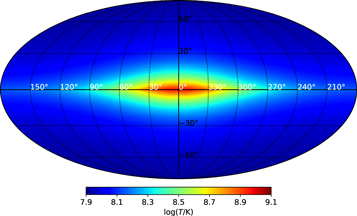
Figure 5. The sky map at 1 MHz without absorption.
Download figure:
Standard image High-resolution imageWith the cylindrical emissivity model and the NE2001 free-electron distribution, one can construct maps with free–free absorption. In Figure 6, we plot the sky map with absorption using the NE2001 fiducial parameters. As one can see in these figures, at the lower frequencies the absorption becomes very significant. In particular, the absorption is strongest along the Galactic plane, and as a result the Galactic disk is darker than high Galactic latitude regions at the lower frequencies. This is in stark contrast with observations at higher frequencies and with the model map without absorption (see Figure 3), where the Galactic disk is the brightest part of the sky.

Figure 6. The ultralong-wavelength sky maps at 10, 3, and 1 MHz, respectively (from top to bottom), for the fiducial NE2001 parameters (F1 = 0.18). Note in this cylindrical model the features from nearby sources such as Loop I and the NPS are not included.
Download figure:
Standard image High-resolution imageHow do these maps compare with the observation? The data at this low-frequency range are scarce, but there are some global spectrum measurements, i.e., the average spectrum for the whole or a large part of the sky. In Figure 7 we plot the global spectrum derived from averaging the brightness of the maps of our model, together with some observational data points. The data were taken by the IMP-6 satellite (filled circles; Brown 1973) and the RAE-2 satellite (upward and downward triangles; Cane 1979). Besides the instrumental differences, the differences between the measurements may be due partly to the different sky areas being averaged over for the two satellites (Keshet et al. 2004). The models are plotted as curves, including the absorption-free case (dotted–dashed line), the extragalactic source (dots), the fiducial NE2001 model (F1 = 0.18, cyan dashed line), and a model with enhanced fluctuations (F1 = 3.0, orange solid line; see discussion below). Compared with the data, we find that the sky brightness below ∼3 MHz is overpredicted when using the NE2001 fiducial fluctuation parameter for the thick disk (F1 = 0.18), as shown by the cyan dashed curve. This has already been noticed by several earlier works (e.g., Peterson & Webber 2002; Webber et al. 2008).
Some works (Gaensler et al. 2008; Sun et al. 2008) show that the scale height of the thick disk could be twice the default value used in NE2001. This would in principle enhance the free–free absorption. However, adopting a larger scale height of 1.8 kpc, as compared to the default 0.97 kpc, results in a decrement of the mean sky brightness by only 11% at 1 MHz, because a large fraction of the sky radiation is from high Galactic latitude regions that are not influenced much by the increase of disk thickness.
Now there are some large uncertainties in the data itself, but the downturn of the spectrum below ∼3 MHz seems robust. If we take the data points below 3 MHz at face value, a possible solution of this discrepancy is that there may be small-scale structures not modeled in the current electron distribution model that enhance the absorption. In order to reach consistent results with the low-frequency observations at ≲3 MHz, one can enhance the absorption by adopting larger fluctuation parameters for the Galactic diffuse components or alternatively by adopting a softer spectral index at lower frequencies. Since the thick disk has the largest influence on the global mean sky brightness, we test the model in which the thick disk has a larger fluctuation parameter of F1 = 3.0, while keeping other parameters the same as the NE2001 fiducial values. Note that the fiducial value of this fluctuation parameter is F1 = 0.18 in NE2001, so the optical depth is enhanced by more than 15 times. The result is the solid curve in Figure 7, which now agrees with the observational data below 3 MHz. The corresponding maps are shown in Figure 8, for frequencies 10, 3, and 1 MHz.

Figure 7. The mean sky brightness in our models (curves) and in observations (points). The dashed–dotted line is the absorption-free sky brightness, the dashed line is the absorption-included sky brightness with F1 = 0.18 in the NE2001 model, and the solid line is the absorption-included sky brightness with F1 = 3.0. The data points are from IMP-6 (filled circles), RAE-2 (triangles), and the maps used to derive the spectral index (stars). As a comparison we plot the extragalactic radiation (Equation (13)) by a dotted line.
Download figure:
Standard image High-resolution imageThe maps in Figures 6 and 8 begin to show differences at 3 MHz, and the two 1 MHz maps are quite different. For the 1 MHz map, in Figure 8 one can see huge shadows of the spiral arms and the Galactic center component in the sky map (the blue–cyan regions at the leftmost and rightmost parts and near the center). Note that the spiral arms not only have higher WIM density than the gap between them, but also are more crowded with discrete H ii regions (Paladini et al. 2004) and their extended envelopes. They produce especially prominent large-scale shadows even at higher frequencies, as has been recognized much earlier (Bridle 1969; Roger et al. 1999; Guzmán et al. 2011). On the other hand, for regions near the Galactic pole, and at some voids, the absorption is much weaker. Such directions would be recommended for detecting extragalactic sources. There are some dark spots, most of which are near the Galactic plane. They are H ii regions around massive stars or SNRs, with enhanced absorption. For example near the Galactic plane at l ∼ 270°, there is the Gum Nebula. It is an ancient SNR with a distance between 200 pc and 500 pc (Woermann et al. 2001). So far, we have not taken into account the radiation from these sources themselves, so the brightness at their locations may be underestimated in such models.
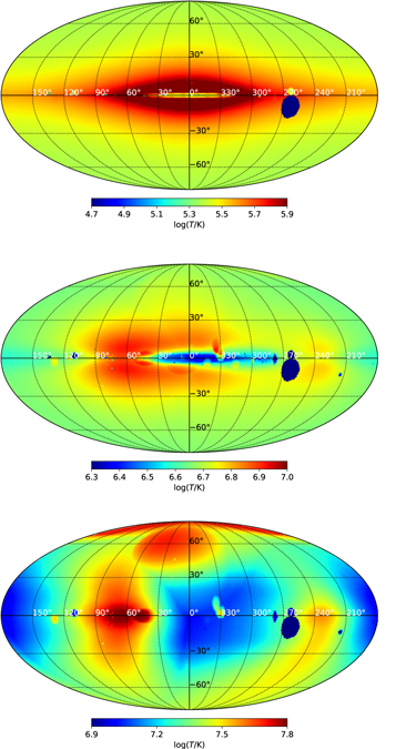
Figure 8. Same as Figure 6, but for a higher fluctuation parameter F1 = 3.0.
Download figure:
Standard image High-resolution imageThe IMP-6 satellite has detected maximum radiation from directions near the Galactic poles at frequencies between 0.13 and 2.6 MHz (Brown 1973), and the modulation index (defined as the ratio between the maximum flux minus the minimum flux and the maximum flux plus the minimum flux) is ∼15% at 1 MHz. The satellite has a poor resolution of ∼100° however. We confirmed that if we smooth our 1 MHz map by a window with FWHM ∼100°, the modulation index is ∼20%. Qualitatively, IMP-6 is in line with our prediction that at ultralong wavelengths, the Galactic plane becomes darker because of the absorption, leaving brighter regions at high Galactic latitudes. However, our smoothed map shows a darker Galactic plane and brighter Galactic poles also significantly modulated by the projected spiral arms, so the direction of the maximum-flux pole is shifted from the Galactic poles. It is not clear if the anisotropy seen by IMP-6 has other causes.
Because of the free–free absorption, the sky radiation observed at ultralong wavelengths would be dominated by nearby sources. As the frequency increases, more and more contribution will be gained from further sources. Therefore, by combining observations at various frequencies, ultralong-wavelength observations provide a 3D tomography tool for measuring the electron distribution and emissivity distribution in the Milky Way. Moreover, with the synchrotron emissivity distribution, one can further derive the cosmic-ray electron spectrum and the magnetic field distribution if gamma-ray observations are analyzed jointly (see Nord et al. 2006; Polderman et al. 2020). In Figure 9, we show maps of the critical distance d50, within which about 50% of the radiation we observe is emitted. Here we adopt a thick-disk fluctuation parameter of F1 = 3.0, and from left to right, we show the results for 10, 3, and 1 MHz. For each line of sight, by comparing the observed specific intensities at different frequencies, one can derive the contribution from different distances.

Figure 9. The half-brightness distance for 10, 3, and 1 MHz, respectively (from left to right).
Download figure:
Standard image High-resolution imageWe also show the optical depth from the Z-axis and Y-axis perspectives in Figure 10. On the Galactic plane, the shape of the local optical depth distribution is irregular, with obvious anisotropy, as well as raylike features due to the nearby ISM distribution. On larger scales, the electron density increases rapidly toward the inner Galaxy region, forming a fanlike structure. From the side view, we can see there are high-transparency cones above and below the Galactic plane. The overall structure is what we would expect: there is more opacity toward the inner region of the Galaxy, but the local ISM could have significant impact.
3.2. Nonsymmetric Variations
The model discussed above is based on an emissivity model with cylindrical symmetry with respect to the Galactic center. For practical usage, it is desirable to have mock sky maps that have nonsymmetric brightness temperature variations. We therefore consider a model that includes such variations, given by

The emissivity fluctuations Δ(ν, R, Z, ϕ, s) are of course very poorly known at present, so we adopt an approximate approach as shown below. The cylindrical absorption-free sky brightness temperature is

and the absorption-included sky brightness temperature is

A "transmittance" for each line of sight is defined as

We then assume that the nonsymmetric temperature variations have the same transmittance as R1 defined above; therefore, instead of looking for a Δ in Equation (23), we directly derive the nonsymmetric variations by

where  is the difference between the extrapolated sky map (using Equation (15)) and the cylindrical
  . Note that for some large-scale features on the sky, this may not be a good approximation. For example Loop I is more likely to be a nearby object (Dickinson 2018); therefore R1 should be higher than the average. We leave this for future work.
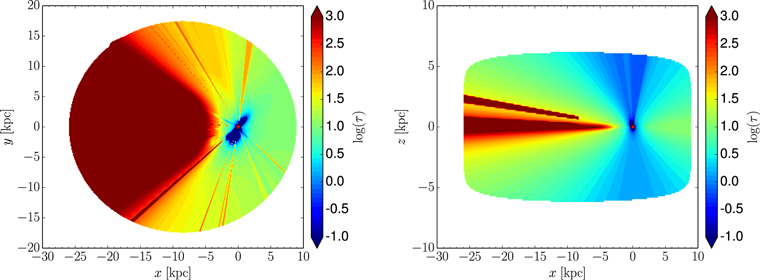
Figure 10. The optical depth distribution at 1 MHz as viewed from the Earth, projected along the Z-axis (left) and Y-axis (right) of the Galactic coordinates. The location of our Sun is marked by a star symbol.
Download figure:
Standard image High-resolution imageWe add these fluctuations to the cylindrical symmetry model sky maps and the results are shown in Figure 11. In Figure 12, we also show the evolution of Galactic absorption in frequencies of 10 to 0.1 MHz. We compare our generated map at 10 MHz with the observed map by Caswell (1976) at the same frequency. In the common sky region, the relative mean deviation is 18.6%. We also compare our generated map at 22 MHz with the observed one by Roger et al. (1999)—the mean relative difference is 19.2%.

Figure 11. The sky maps at 10, 3, and 1 MHz, respectively, from top to bottom. Here we add fluctuations to the cylindrical symmetry model, and F1 = 3.0 is adopted.
Download figure:
Standard image High-resolution imageFigure 12. A still image from an animation of the evolution of the sky maps from 10 MHz to 0.1 MHz. This 12 s animation advances in 0.1 MHz decrements.
(An animation of this figure is available.)
Download figure:
Video Standard image High-resolution image3.3. Frequency Dependence of the Spectral Index
So far we have only considered models with constant spectral indices for both the extragalactic background and Galactic synchrotron radiation. However, the spectral index may vary with frequency. For example, the energy spectrum of interstellar cosmic-ray electrons derived from the combination of PAMELA observations at near-Earth space and Voyager observations at distant space (≳100 au) can be described by a broken power-law form, with a broken point at ∼0.1–1 GeV (Potgieter & Nndanganeni 2013; Bisschoff et al. 2019). Assuming a typical interstellar magnetic field ∼5 μG, then the broken point corresponds to synchrotron critical frequency ∼1–100 MHz. Inspired by this, in this section we investigate a model in which the synchrotron spectral index depends on frequency.
The frequency dependence of the spectral index is not yet confirmed in current observations at ≳10–22 MHz. To proceed, we tentatively assume the following frequency dependence for the spectral index, for both Galactic radiation and the extragalactic background:

where β0 = −2.58 and −2.51 is the constant spectral index in our fiducial model for the extragalactic background and Galactic radiation, respectively, and ν1 is a critical frequency—for ν ≫ ν1, β ≈ β0; for ν ≪ ν1, β ≈ β0 + β1. For simplicity we adopt the same β1 = 0.7 and ν1 = 1.0 MHz for both Galactic radiation and the extragalactic background.
The absorption-included sky maps with a frequency-dependent spectral index are shown in Figure 13. Here we adopt F1 = 0.18, as the default of NE2001. Comparing them with Figure 8, we find that although the mean sky brightness is similar, the morphology is rather different, especially at lower frequencies. Ultralong-wavelength observations would provide necessary information to distinguish between these two models.

Figure 13. Same as Figure 6; however, here the synchrotron radiation has a frequency-dependent spectral index as in Equation (28).
Download figure:
Standard image High-resolution imageWith this frequency-dependent spectral index, the tension on the fluctuation parameter discussed in Section 3.1 can be mitigated; see Figure 14, where we plot the mean sky brightness in this model. Even for the fiducial fluctuation parameter F1 = 0.18 in NE2001, the spectrum is consistent with the ultralong-wavelength observations.

Figure 14. The mean sky brightness as a function of frequency in frequency-dependent and direction-dependent models. The dotted–dashed and solid curves show the absorption-free and absorption-included sky, respectively, for a frequency-dependent spectral index and a direction-dependent spectral index.
Download figure:
Standard image High-resolution image3.4. Spatial Variations of the Spectral Index
The spectral index could also have spatial variations. However, at low frequency only the Haslam 408 MHz map covers the full sky. To derive the full-sky spectral index map, we first generate a spectral index map by combining the Haslam 408 MHz map with the LWA maps, and another one by combining the 408 MHz map with the Guzman 45 MHz map. These two maps are incomplete around the south and north celestial poles, respectively, but for sky regions common to both maps, the two maps show similar structures, and the difference is about a 13.6% standard deviation. We produce a combined map by connecting these two spectral index maps by a smooth function. The spectral index at decl. δ is
where βG1 is the spectral index derived by the Haslam 408 MHz map and LWA maps, while βG2 is the spectral index derived by the Haslam 408 MHz map and Guzman 45 MHz map. When δ ≫ δ0, we have β ≈ βG1, and when δ ≪ δ0, β ≈ βG2. We take δ0 = −15° and A = 1.7.
All maps used here are smoothed by a Gaussian beam with FWHM = 5°. The resulting spectral index map is shown in Figure 15. At the Galactic plane the spectrum slope is shallower than the higher Galactic latitude, and the southern sky is also shallower than the northern sky. Note here the spectral index is for the frequency range of a few tens of megahertz to 408 MHz, where the free–free absorption is still small except for dense H ii regions, so it reflects the intrinsic emission spectrum.
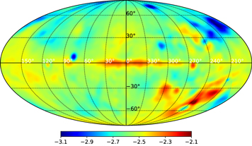
Figure 15. The spectral index map obtained by combining the Haslam 408 MHz map with the LWA and Guzman maps.
Download figure:
Standard image High-resolution imageWe then model the emissivity as
It is formally the same as Equation (17), except that now βG is allowed to vary with direction (direction-dependent), and the value is taken from the spectral index map obtained above. Using the emissivity given above, and adding the free–free absorption and small-scale fluctuations (here we also adopt F1 = 3.0), we finally obtain the map shown in Figure 16. Compared with that in Figure 11, the overall brightness is higher in these maps, because the pixels with steeper spectral indices become brighter when extrapolated to the lower frequencies.
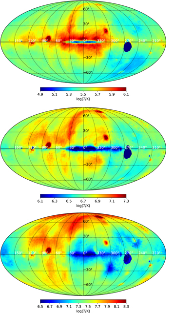
Figure 16. Sky maps at (from top to bottom) 10, 3, and 1 MHz for the model with a direction-dependent spectral index.
Download figure:
Standard image High-resolution imageThe mean sky brightness temperature is also plotted in Figure 14. In this model, for the same absorption strength (F1 parameter) the sky brightness temperature is higher than the constant spectral index model, at frequencies below ∼3 MHz. As we see in Figure 15, the spectrum slope at higher Galactic latitude is steeper than the lower Galactic latitude, and as a result, the absorption-free brightness at high Galactic latitude is higher than that in the constant spectral index model. In addition, the free–free absorption at higher Galactic latitude is weaker. Consequently, the ultralong-wavelength sky is brighter in the direction-dependent spectral index model.
3.5. Absorption from EHEs
As noted above, the NE2001 model with its fiducial parameters may predict inadequate absorption to produce the observed downturn in the global radio spectrum. To overcome this difficulty we considered adopting a larger fluctuation parameter, i.e., by assuming there are more small-scale fluctuations in the WIM. We now consider another, more physical solution to this problem.
NE2001 includes 175 known H ii objects (SNRs or H ii regions) with enhanced electron densities ranging from 0.01 to 40 cm−3. Most of them have density ∼0.5 cm−3 at the center, and are modeled with Gaussian profiles of width ∼ 0.01 kpc. Of course this is not a complete list; there should be many more SNRs, probably between 1000 and 10,000 (Berkhuijsen 1984), and more H ii regions (the Wide-field Infrared Survey Explorer mission has already detected more than 8000; see Anderson et al. 2014). H ii regions could be small and dense (compact or classical H ii regions), or large and diffuse (diffuse H ii regions; e.g., Lockman et al. 1996; Anderson et al. 2018). Around the classical H ii regions there could be EHEs, with sizes extending to ∼0.05–0.2 kpc, density ∼0.5–10 cm−3, and temperature 3000–8000 K, as found by low-frequency radio recombination lines (Anantharamaiah 1985a, 1985b, 1986; Roshi & Anantharamaiah 2001) or absorption of the radio continuum toward SNRs (Kassim 1989; Lacey et al. 2001).
We now consider the contribution to free–free absorption if more absorbers are included, to see if they can account for the downturn of the observed global radio spectrum at ≲3–5 MHz. Although the classical H ii region is opaque to low-frequency radio flux, it is difficult for them to significantly reduce the global spectrum because their volume filling factor is too small, so here we focus only on EHEs.
We assume the spatial distribution of EHEs in the Milky Way has a form similar to that of SNRs (Strong & Moskalenko 1998):
where Zs = 0.2 kpc, η = 1.25, and ξ = 3.56 as constrained by the Fermi Galactic gamma-ray observations (Trotta et al. 2011). The normalization factor q0 is set by

where NEHE is the total number of EHEs in the Milky Way, and is treated as a free parameter here.
We make random realizations of the EHEs that follow the spatial distribution of Equation (31), and further assume that their size follows a log-normal distribution, with central value  and variance
  , and is limited in the range 0.05–0.2 kpc. For simplicity, we model them with sharp edges, and within the edge the electron density is 1.0 cm−3, to be consistent with the typical EHEs. We adopt the same density for all mock EHEs. Regarding the total number, we adopt NEHE = 20,000. We artificially remove one EHE that occasionally encompasses our Sun; it will not influence the statistics of the sample.
In the top panel of Figure 17 we plot the free–free absorption optical depth to extragalactic sources, purely by our mock EHEs, at 1 MHz. We then replace the H ii clump list in NE2001 with these mock EHEs, and then recalculate the sky map. For all other parameters we still use the fiducial values in NE2001, because we want to see if the mock EHEs could account for the downturn on the global radio spectrum without increasing the WIM absorption.
Figure 17. Top: the free–free optical depth of the mock EHEs. Middle: the sky map. Bottom: the global radio spectrum.
Download figure:
Standard image High-resolution image
In the middle panel of Figure 17 we plot the 1 MHz sky map, and in the bottom panel we plot the global spectrum. For both of them the absorption from the WIM and mock EHEs is involved. In the bottom panel we also plot the global spectrum if only the absorption from mock EHEs is involved. Clearly, the mock EHEs cover ∼80% of the sky area and can absorb the ultralong-wavelength signal efficiently. However, when we look through the shape of the global spectrum shown in the bottom panel of Figure 17, we find that the predicted shape does not agree with the observations well.
In our random sample, all EHEs are opaque to radio signals at 1 MHz and they occupy ∼80% of the sky area. Therefore ∼20% of the flux leaks between gaps in the EHEs and can be detected unabsorbed. That is to say, the observed global spectrum is

where I0 is the global spectrum without EHE absorption, and fsky is the sky coverage of the EHEs (not the volume filling factor, so it could be close to 1). Because here fsky ∼ 1, 1 − fsky ≪ 1. When ν ≫ 1 MHz, the optical depth is still not that large. As a result the second term of the right-hand side (RHS) dominates the observed global spectrum. When ν ∼ 1 MHz, the EHEs are opaque enough so that ![${I}_{0}(\nu )\exp [-\tau (\nu )]\sim 0$](https://content.cld.iop.org/journals/0004-637X/914/2/128/1/apjabf55cieqn24.gif) and the first term of the RHS dominates. Therefore I(ν) shows a complex trend with decreasing frequency, as shown by the bottom panel of Figure 17. The WIM absorption would change the I0(ν), so it also changes the behavior of I(ν), but not significantly; see the difference between the curves with and without the WIM in the bottom panel of Figure 17.
and the first term of the RHS dominates. Therefore I(ν) shows a complex trend with decreasing frequency, as shown by the bottom panel of Figure 17. The WIM absorption would change the I0(ν), so it also changes the behavior of I(ν), but not significantly; see the difference between the curves with and without the WIM in the bottom panel of Figure 17.
We further check that, to produce the downturn in such a model, we must have one low-density EHE encompassing the Sun. If our Sun is inside an EHE with a typical density of ∼0.1 cm−3, we can get the global spectrum to turn over at ∼3–5 MHz and be consistent with observations. However, we note that it is known that the Sun resides in a region known as the Local Bubble, which has much lower density than the abovementioned EHE (Frisch et al. 2011). So if there are many EHEs they could indeed affect the global radio spectrum significantly, but to produce a downturn consistent with observations, while also being consistent with the observed local density around the Sun, is still difficult.
4. Conclusions
In this work, we have developed an ultralong-wavelength radio sky model that is valid below ∼10 MHz. We first derive a cylindrical emissivity from the observed all-sky map at 408 MHz, extrapolate it to ultralong wavelength using a power-law form, and then add the free–free absorption by the Galactic diffuse free electrons and some small-scale dense H ii regions. The spectral index of the power law is derived from observed multiwavelength radio maps and the Galactic free-electron distribution is from the NE2001 model.
We found that if we use a constant spectral index βG = −2.51 for Galactic synchrotron radiation and adopt the fiducial fluctuation parameter for thick disk (F1 = 0.18) in the Galactic electron model NE2001, we would overpredict the mean sky brightness at ≲3 MHz as compared with the observations by space satellites. The observed mean sky brightness spectrum (the specific intensity) turns over at ∼3 MHz. To solve the problem, either the Galactic diffuse electrons have much larger small-scale fluctuations than modeled by NE2001, or the intrinsic synchrotron radiation spectrum itself has a shallower slope at ≲3 MHz. We investigated both solutions. The morphologies of predicted sky maps in these two cases are quite different; therefore, in the future a high-resolution ultralong-wavelength sky survey could potentially distinguish between them. Moreover, we investigated a model in which the spectral index depends on direction.
In particular, we found that, at ultralong wavelengths, the Galactic plane would be darker than higher Galactic latitude regions. Moreover, one can see the shadows of spiral arms from the sky map, particularly at frequencies as low as ∼1 MHz. From the multifrequency sky maps one can obtain the 3D information of the Galactic diffuse electrons and emissivity distribution.
Our model would be a useful tool for designing the upcoming ultralong-wavelength experiments. The first generation of lunar-orbit and lunar-surface-based interferometers would have a limited number of antennas; hence a reasonable input sky model would be crucial. Our model can be used to test whether these interferometers can successfully and accurately recover the ultralong-wavelength sky, which has a complex brightness distribution and changes dramatically with frequency. Moreover, when new observational data is available, our model can generate low-frequency sky maps, which can be used for imaging deconvolution.
We have made our model  publicly available, including the source code, the maps at different frequencies for different models, and some animated figures. They can be downloaded at 10.5281/zenodo.4454153.
We thank Dr. Jiaxin Wang for helpful discussions. This work is supported by the CAS Strategic Priority Research Program XDA15020200; National Natural Science Foundation of China (NSFC) grants 11973047, 11633004, and 11653003; and the NSFC–ISF joint research program, No. 11761141012. B.Y. also acknowledges support from the NSFC–CAS joint fund for space scientific satellites (No. U1738125) and the CAS Bairen program.
Appendix: The Ultralong-wavelength Sky Model Software
A.1. The Structure of the Code
We developed a Python code package named Ultralong-wavelength Sky Model with Absorption (ULSA) to generate the sky map at very low frequencies, taking into account the free–free absorption effect by free electrons in both discrete H ii clumps and the WIM. The code first sets up the model for the Galactic emissivity distribution by fitting available observational data at higher frequencies, and the free-electron distribution, then generates the absorbed full-sky map. The code files are organized as follows (all under the ULSA directory), with brief explanations in italics:
- 1.spectral_index_fitting/ Spectral indices, three models are provided. spectral_index_constant.py spectral_index_frequency_dependent.py spectral_index_direction_dependent.py
- 2.emissivity_fitting/ Set up emissivity model. produce_data_for_fitting.py Preprocess the data for emissivity fitting, removing nearby structures "NPS" and "Loop I." fit_emissivity_params.py Fit the emissivity parameters.
- 3.NE2001/* The Galactic electron model.
- 4.sky_map/ Make the sky map. produce_absorbed_sky_map.py
The computations are done in the following three steps:
- 1.Spectral Index Parameter Fitting. As described in the main text, we have developed three models with different spectral indices: (i) a constant spectral index, (ii) a frequency-dependent spectral index, and (iii) a direction-dependent spectral index. The user may choose one of these. In this step the code produces the spectral index parameters for use in the next step. Once this is done, the sky map can be extrapolated from 408 MHz to lower frequencies.
- 2.Galactic Emissivity Model Construction. We then derive the emissivity model parameters using the code in the emissivity_fitting/ directory. First, we preprocess the data by removing local structures such as the NPS and Loop I from the 408 MHz map; then the emissivity model parameters are obtained by fitting this map.
- 3.Low-frequency Sky Map Generation. Finally, the sky map is generated with the emissivity model constructed above and the free–free absorption effect is computed using the NE2001 model.
To run the code, one can simply call the absorption_JRZ function, which serves as the drive routine, with appropriate choices of various parameters:
- >>> from ULSA.sky_map.produce_absorbed_sky_map import absorption_JRZ
- >>> f = absorption_JRZ(v, nside, index_type, distance, using_raw_diffuse, using_default_params,
- critical_dis,output_absorp_free_skymap).mpi()
The parameters in the command are as follows:
- 1.v (float): the frequency in megahertz for the output map.
- 2.nside (int): the Healpix NSIDE value for the sky map.
- 3.index_type (str): the spectral index modeling option, one of constant_index, freq_dependent_index, and direction_dependent_index.
- 4.distance (kpc): maximum integration distance along line of sight; the default is set to 50 kpc.
- 5.using_raw_diffuse (bool): if False, the data will be smoothed by the Gaussian kernel; otherwise the raw data will be used.
- 6.v_file_dir (dict): a dictionary structure used to specify additional input map data. Specifies the frequency of the map by the dictionary key, and the relative path of the map data as the dictionary value. The input sky map file should be in HDF5 format, such as {XX:"/dir/xxx.hdf5"}. If None, the spectral index is calculated with the existing data.
- 7.using_default_params (bool): if True, it uses the default spectral index value in the code, or recalculates the spectral index value if False.
- 8.input_spectral_index (array): one can specify the spectral index value by putting in an array containing the spectral index map in the direction-dependent case, or an array containing one element for the constant and frequency-dependent cases.
- 9.params_408 (list): the emissivity model parameters (A, R0, α, Z0, and γ) obtained by fitting the Haslam 408 MHz sky map. If this parameter is omitted, the values given in Table 1 will be used as defaults. One can also specify these parameters directly by putting in the values, or force the code to refit by setting it to [0.,0.,0.,0.,0.].
- 10.critical_dis (bool): if True, it calculates the half-brightness distance; otherwise this is not calculated.
- 11.output_absorp_free_skymap (bool): if True, it produces an absorption-free sky map at frequency v as well.
The function returns a 2D matrix, the first column is the Healpix pixel number, and the second column gives the corresponding sky map. One can then plot this map using healpy.mollview. The default coordinate system is set to the Galactic coordinate system, but one can transform it to the equatorial coordinate system by calling the Healpix function f.change_coord(m,["G", "C"]). See the healpy documentation for more information. Additionally, some results are automatically rendered as an HDF5 file. The map is saved in a file with a name of the form freqMHz_sky_map_with_absorption.hdf5, where freq is the frequency in megahertz. This file contains two keys that are respectively named "spectral_index" for the spectral index map and "data" for the sky map at the given frequency.
An absorption-free sky map is computed as an intermediate result though not saved automatically, but if the parameter output_absorp_free_skymap is set as True, it will be saved in a file named in the format freqMHz_absor p_free_skymap.hdf5. Moreover, the half-brightness distance will be computed and saved as freqMHz_critical_dist.hdf5 if the parameter critical_dis is set as True.
A.2. An Example of Using the Code
In the example shown below, sky maps are produced at 1, 2, ... 10 MHz with the constant spectral index model.
A.3. Adding New Input Map Data
All the observation maps used in this work are under the directory obs_sky_data/; one can also add new map data (e.g., at additional frequencies) there. The map file should be in the HDF5 format, with the first column indicating the HEALPIX pixel number, and the second column the sky temperature values in equatorial coordinates. Most observed data in their original form are in these coordinates; if not, one must convert them into equatorial coordinates. To use such new data, first, put the new data under obs_sky_data/; then, when calling the function, register the new data by a dictionary whose key is the frequency of this new input map, and the value is the path relative to obs_sky_data/. For example, if there is a new map at 22 MHz, one first creates a file 22MHz_sky_map.hdf5, putting it under obs_sky_data/22MHz/22MHz_sky_map.hdf5; then, when calling the absorption_JRZ function, provide v_file_dir={22:''/22MHz/22MHz_sky_map.hdf5''}. The code will then add the new data when calculating the spectral index.
Footnotes
- 5
At such low frequencies, the resolution is limited by scattering in the ISM and interplanetary medium. This angular scattering limit is roughly at the arcminute level at 1 MHz and roughly scales with ∝ ν−2 (see Jester & Falcke 2009).
- 6
- 7
Using Equation (2) and the electron model in Section 2.5, we check that at this frequency, for most of the sky regions the free–free absorption is negligible, except at a very thin plane with b ∼ 0° and near the Galactic center, where the optical depth could be up to ∼1, so it is safe to include these low-frequency observations when constructing the absorption-free map.