


Abstract
Spectroscopic detection of narrow emission lines traces the presence of circumstellar mass distributions around massive stars exploding as core-collapse supernovae. Transient emission lines disappearing shortly after the supernova explosion suggest that the material spatial extent is compact and implies an increased mass loss shortly prior to explosion. Here, we present a systematic survey for such transient emission lines (Flash Spectroscopy) among Type II supernovae detected in the first year of the Zwicky Transient Facility survey. We find that at least six out of ten events for which a spectrum was obtained within two days of the estimated explosion time show evidence for such transient flash lines. Our measured flash event fraction (>30% at 95% confidence level) indicates that elevated mass loss is a common process occurring in massive stars that are about to explode as supernovae.
Export citation and abstract BibTeX RIS
1. Introduction
Massive stars (M > 8 M⊙) explode as core-collapse supernovae (CC SNe; Smartt 2015; Gal-Yam 2017), and often experience mass loss from their outer layers due to stellar winds, binary interaction, or eruptive mass-loss events (see, e.g., Smith 2014 and references within). The mass lost by these stars forms distributions of circumstellar medium (CSM). The CSM properties depend on the mass-loss rate, the velocity of the flow, and the duration of the process.
When a massive star surrounded by CSM explodes as a CC SN, signatures of the CSM may manifest as spectroscopic features with a narrow width reflecting the mass-loss velocity, which is typically low compared to the expansion velocity of the supernova ejecta (a few hundreds of km s−1 versus ≈ 10,000 km s−1). Such features often persist for more than two days from the explosion, which sets the extent of the material to >1014 cm, a scale far above that of the atmospheres of the largest supergiants. In Type IIn SNe (e.g., Schlegel 1990; Filippenko 1997; Kiewe et al. 2012; Taddia et al. 2013; Gal-Yam 2017; Nyholm et al. 2020), narrow hydrogen lines persist for weeks to years after explosion, indicating an extensive CSM distribution. Type Ibn events (e.g., Hosseinzadeh et al. 2015; Pastorello et al. 2016; Gal-Yam 2017; Karamehmetoglu et al. 2019) show strong emission lines of helium, suggesting recent mass loss from stripped progenitors. In both Types IIn and Ibn, there is evidence that in at least some cases, the mass-loss is generated by precursor events, prior to the SN explosion (e.g., Foley et al. 2007; Pastorello et al. 2007; Ofek et al. 2013, 2014; Strotjohann et al. 2021).
If the CSM extension is confined to a relatively compact location around an exploding star, the explosion shock-breakout flash may ionize the CSM. The resulting recombination emission lines will be transient, persisting only until the SN ejecta overtakes and engulfs the denser parts of the CSM (supernovae with "flash-ionized" emission lines; Gal-Yam et al. 2014). Such events later evolve spectroscopically in a regular manner, e.g., presenting photospheric spectra with broad P-Cygni line profiles.
Several serendipitous observation of such "flash features" in early supernova spectra were made over the years (e.g., Niemela et al. 1985; Garnavich & Ann 1994; Quimby et al. 2007). We define flash features here as transient narrow emission lines (of the order of ≈ 102 km s−1) of highly ionized species (e.g.,: He ii, C iii, N iii, N iv) in the early phases of the supernova event (in general, less than a week from the estimated explosion). Gal-Yam et al. (2014) presented very early observations of the Type IIb SN 2013cu, and noted that such flash features could be routinely observed by modern high-cadence SN surveys. These features reveal the composition of the pre-explosion mass loss, and hence probe the surface composition of the progenitor star, which is hard to measure by other means. This work motivated additional studies on such flash objects. For example, Yaron et al. (2017) presented a time-series of early spectra which they used to constrain the CSM distribution around the spectroscopically normal SN 2013fs. They show that the CSM was lost from the progenitor during the year prior to its explosion. Hosseinzadeh et al. (2018) studied the low-luminosity Type II event, SN 2016bkv, which showed early flash ionization features. They suggest that its early light-curve bump implies a contribution from CSM interaction to the early light curve. Such interpretations motivate the systematic study of early light curves of Type II SNe with flash features to distinguish between possible contributions of CSM interaction versus shock cooling emission, for example, by testing the correlation of peak luminosity and/or rise time with the existence of flash features. Several theoretical investigations also focused on such events (e.g., Groh 2014; Dessart et al. 2017; Moriya et al. 2017; Kochanek 2019; Boian & Groh 2020).
A systematic study of such transient signatures of CSM around SN II progenitor stars has been limited by the challenge of routinely observing CC SNe early enough (typically within less than a few days from explosion), before these features disappear. Khazov et al. (2016) conducted the first sample study of flash ionization features in Type II SNe using data from the PTF and iPTF surveys. They gathered twelve objects showing flash ionization features and estimated that more than ∼20% of SNe II show flash ionization features, although their analysis was limited by the heterogeneity of their data.
Routine observations of young ("infant") SNe was one of the main goals of the ZTF survey (Gal-Yam 2019; Graham et al. 2019). Here, we present our systematic search and follow-up observations of infant Type II SNe from ZTF. We use a sample of 28 events collected during the first year of ZTF operation to place a lower limit on the fraction of SN progenitor stars embedded in CSM. Ten of these objects were spectroscopically observed within two days of the estimated explosion.
In Section 2, we describe the properties of our infant SN survey and the construction of our sample of SNe II. In Section 3 we present our analysis, in Section 4 we discuss our findings, and we conclude in Section 5.
2. Observations and Sample construction
2.1. Selecting Infant SNe from the ZTF Partnership Stream
The Zwicky Transient Facility (ZTF) is a wide-field, high cadence, multiband survey that started operating in 2018 March (Bellm et al. 2019; Graham et al. 2019). ZTF imaging is obtained using the Samuel Oschin 48" Schmidt telescope at Palomar observatory (P48). ZTF observing time is divided into three programs: the public (MSIP) 3 day all-sky survey, partnership surveys, and Caltech programs. This paper is based on data obtained by the high-cadence partnership survey. As part of this program, during 2018, extragalactic survey fields were observed in both the ZTF g- and r-bands 2–3 times per night, per band. New images were processed through the ZTF pipeline (Masci et al. 2019), and reference images, built by combining stacks of previous ZTF imaging in each band, were then subtracted using the Zackay et al. (2016) image subtraction algorithm (ZOGY). A 30 s integration time was used in both g- and r-band exposures. A 5σ detection limit is adopted for estimating the limiting magnitude, typically reaching ∼20.5 mag in r-band in a single observation.
We conducted our year-1 ZTF survey for infant SNe following the methodology of Gal-Yam et al. (2011). We selected potential targets via a custom filter running on the ZTF alert stream using the GROWTH Marshal platform (Kasliwal et al. 2019). The filter scheme was based on the criteria listed in Table 1.
Table 1. Filter Criteria Selecting Infant SN Candidates
| Stationary | Reject solar system objects using apparent motion |
|---|---|
| Recent limit | Require a non-detection limit within <2.5 days from the first detection |
| Extragalactic | Reject alerts within 14 degrees from the Galactic plane |
| Significant | Require a ZOGY score of >5 |
| Stellar | Require a SG (star-galaxy) score a of <0.49 |
Note.
a This parameter indicates whether the closest source in the PS1 catalog is stellar. See https://zwickytransientfacility.github.io/ztf-avro-alert/schema.html.Download table as: ASCIITypeset image
Alerts that passed our filter (typically 50–100 alerts per day) were then visually scanned by a duty astronomer, in order to reject various artefacts (such as unmasked bad pixels or ghosts) and false-positive signals (such as flaring M stars, CVs and AGN). Most spurious sources could be identified by cross-matching with additional catalogs, e.g., WISE IR photometry (Wright et al. 2010) to detect red M stars, the Gaia DR2 catalog (Gaia Collaboration et al. 2018), and catalogs from time-domain surveys such as the Palomar Transient Factory (PTF; Law et al. 2009) and the Catalina Real-Time Survey (CRTS; Drake et al. 2014) for previous variability of CVs and AGN.
Due to time-zone differences, our scanning team (located mostly at the Weizmann Institute in Israel and the Oskar Klein Center (OKC) in Sweden) could routinely monitor the incoming alert stream during the California night time. We aimed at triggering spectroscopic follow-up of promising infant SN candidates within hours of discovery (and thus typically within <2 days from explosion), as well as Swift, (Gehrels et al. 2004) Target-of-Opportunity (ToO) UV photometry.
2.2. Sample Construction
Figure 1 shows the SN Type distribution among the ∼2500 spectroscopically confirmed SNe gathered by ZTF between 2018 March and December. About 34% are core-collapse events, and ∼62% of those are of Type II. We can only place statistically meaningful constraints on the frequency of flash features among Type II SNe, since these mostly occur in this population. Hence, we choose to study only the SN II population from ZTF year 1.
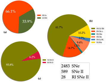
Figure 1. ZTF Spectroscopically confirmed SN discovery statistics during 2018. (a) Most events (66%) are SNe Ia; CC SNe comprise about 34%. (b) The division among CC SN sub-classes (c) The fraction of real infant (RI) SNe II is 6.2% of the total Type II population. NI stands for the Non Infant SN II population (see text).
Download figure:
Standard image High-resolution imageOur infant SN program allowed us to obtain early photometric and spectroscopic follow-up of young SNe. However,we may have missed some relevant candidates.To ensure the completeness of our sample, we, therefore, inspected all spectroscopically classified SNe II (including subtypes IIn and IIb) from ZTF 24 using the ZTFquery package (Rigault 2018). We removed from this sample all events (the large majority) lacking a ZTF non-detection limit within 2.5 days prior to the first detection recorded on the ZTF Marshal. To include events in our final sample, we required that they show a significant and rapid increase in flux with respect to the last non-detection, as previously observed for very young SNe (e.g., Gal-Yam et al. 2014; Yaron et al. 2017). This excludes older events that are just slightly below our detection limit and are picked up by the filter when they slowly rise, or when weather conditions improve. We implemented a cut on the observed rise of Δr or Δg > 0.5 mag with respect to the recent limit in the same band, and labeled all events that satisfy this cut as "real infant" (RI; Figure 1, panel (C)).
All in all, we gathered 43 candidates which fulfilled the RI criteria. Additional inspection led us to determine that 15 candidates were spurious (see Appendix for details). Our final sample (Table 2) thus includes a total of 28 RI Type II SNe, or about 6.2% of all the SNe II found during 2018 by the ZTF survey. During its first year of operation (starting 2018 March), ZTF obtained useful observations for our program during approximately 32 weeks, excluding periods of reference image building (initially), periods dedicated to Galactic observations, and periods of technical/weather closure. We find that the survey provided about one real infant SN II per week.
Table 2. Sample of Real Infant 2018 (28 objects)
| IAU | Internal | Type a | Redshift | Explosion | Error | First | Last Non | First | Telescope/ | Flash |
|---|---|---|---|---|---|---|---|---|---|---|
| Name | ZTF | z | JD Date | Detection | Detection | Spectrum | Instrument | |||
| (SN) | Name | (days) | (days) | (days) b | (days) | (days) | ||||
| 2018grf | 18abwlsoi | SN II (1) | 0.054 | 2458377.6103 | 0.0139 | 0.0227 | −0.8725 | 0.1407 | P60/SEDm | ✓ |
| 2018fzn | 18abojpnr | SN IIb (2) | 0.037 | 2458351.7068 | 0.0103 | 0.0102 | −0.0103 | 0.1902 | P60/SEDm | ⨯ |
| 2018dfi | 18abffyqp | SN IIb (3) | 0.031 | 2458307.2540 | 0.4320 | 0.4320 | −0.4320 | 0.6180 | P200/DBSP | ✓ |
| 2018cxn | 18abckutn | SN II (4) | 0.041 | 2458289.8074 | 0.4189 | 0.0576 | −0.0494 | 0.9406 | P200/DBSP | ⨯ |
| 2018dfc | 18abeajml | SN II (5) | 0.037 | 2458303.7777 | 0.0118 | 0.0213 | −0.9806 | 1.0153 | P60/SEDm | ✓ |
| 2018fif | 18abokyfk | SN II (6) | 0.017 | 2458350.9535 | 0.3743 | −0.0635 | −1.0525 | 1.0525 | P200/DBSP | ✓ |
| 2018gts | 18abvvmdf | SN II (7) | 0.030 | 2458375.1028 | 0.5551 | −0.4688 | −1.3648 | 1.5162 | P60/SEDm | ✓ |
| 2018cyg | 18abdbysy | SN II (8) | 0.011 | 2458294.7273 | 0.2034 | 0.0297 | 0.0147 | 1.6727 | WHT/ACAM | ? |
| 2018cug | 18abcptmt | SN II (9) | 0.050 | 2458290.9160 | 0.0250 | −0.0066 | −0.0670 | 1.7960 | P60/SEDm | ✓ |
| 2018egh | 18abgqvwv | SN II (10) | 0.038 | 2458312.7454 | 0.4351 | 0.9846 | 0.0931 | 1.8236 | WHT/ISIS | ? |
| 2018bqs | 18aarpttw | SN II (11) | 0.047 | 2458246.8133 | 0.0071 | 0.0087 | −0.9926 | 2.0867 | APO/DIS | ⨯ |
| 2018fsm | 18absldfl | SN II (12) | 0.035 | 2458363.4226 | 0.4565 | 0.4564 | −0.4564 | 2.3674 | P60/SEDm | ⨯ |
| 2018bge | 18aaqkoyr | SN II (13) | 0.024 | 2458243.1671 | 0.5180 | 0.5179 | −0.5180 | 2.5169 | P200/DBSP | ⨯ |
| 2018leh | 18adbmrug | SN IIn (14) | 0.024 | 2458481.7505 | 0.9485 | 0.9485 | −0.9485 | 3.6985 | WHT/ISIS | ✓ |
| 2018iua | 18acploez | SN II (15) | 0.042 | 2458439.9877 | 0.9784 | 0.9783 | −0.9783 | 3.7933 | P60/SEDm | ⨯ |
| 2018gvn | 18abyvenk | SN II (16) | 0.043 | 2458385.6198 | 0.0011 | 0.0012 | −0.8565 | 6.1122 | P60/SEDm | ⨯ |
| 2018clq | 18aatlfus | SN II (17) | 0.045 | 2458248.8967 | 0.9564 | 0.9564 | −0.9564 | 6.9274 | P60/SEDm | ⨯ |
| 2018ccp | 18aawyjjq | SN II (18) | 0.040 | 2458263.7743 | 0.1241 | 0.0106 | −0.8684 | 8.1087 | P60/SEDm | ⨯ |
| 2018lth | 18aayxxew | SN II (19) | 0.061 | 2458278.6531 | 0.9154 | 0.0509 | −1.9102 | 8.1589 | Keck/LRIS | ⨯ |
| 2018inm | 18achtnvk | SN II (20) | 0.040 | 2458432.9113 | 0.6895 | 1.9927 | 1.9497 | 9.0137 | P60/SEDm | ⨯ |
| 2018iwe | 18abufaej | SN II (21) | 0.062 | 2458368.8561 | 0.0179 | 0.0179 | −0.0179 | 12.0159 | P60/SEDm | ⨯ |
| 2018fso | 18abrlljc | SN II (22) | 0.050 | 2458357.6987 | 0.8255 | −0.0177 | −0.9157 | 14.0113 | P60/SEDm | ⨯ |
| 2018efd | 18abgrbjb | SN IIb (23) | 0.030 | 2458312.8922 | 0.3938 | 0.8568 | 0.8244 | 14.9388 | P60/SEDm | ⨯ |
| 2018cyh | 18abcezmh | SN II (24) | 0.057 | 2458286.3752 | 0.6050 | 0.4348 | 0.3898 | 16.5678 | P60/SEDm | ⨯ |
| 2018ltg | 18aarqxbw | SN II (25) | 0.048 | 2458241.4360 | 3.4950 | 3.4950 | −3.4950 | 37.5310 | P200/DBSP | ⨯ |
| 2018lti | 18abddjpt | SN II (26) | 0.070 | 2458294.6217 | 0.1224 | 0.1693 | −0.7917 | 40.2333 | P60/SEDm | ⨯ |
| 2018efj | 18abimhfu | SN II (27) | 0.050 | 2458320.6574 | 0.0210 | 0.0096 | −0.9028 | 42.0096 | P60/SEDm | ⨯ |
| 2018cfj | 18aavpady | SN II (28) | 0.047 | 2458256.4531 | 0.4771 | 0.4771 | −0.4771 | 55.0469 | Keck/LRIS | ⨯ |
Notes. (1) Fremling et al. (2018a), (2) Fremling et al. (2018g), (3) Hiramatsu et al. (2018), (4) Fremling & Sharma (2018a), (5) Fremling & Sharma (2018b), (6) Gal-Yam et al. (2018), (7) Fremling et al. (2018b), (8) Fremling & Sharma (2018c), (9) Fremling & Sharma (2018d), (10) Bruch (2020), (11) Bruch (2020), (12) Fremling et al. (2018c), (13) Prentice (2018), (14) Dugas et al. (2019), (15) Bruch (2020), (16) Fremling et al. (2018d), (17) Fremling et al. (2018h), (18) Fremling et al. (2019), (19) Bruch (2020), (20) Fremling et al. (2018e), (21) Bruch (2020), (22) Fremling et al. (2018i), (23) Fremling et al. (2018j), (24) Bruch (2020), (25) Bruch (2020), (26) Bruch (2020) (27) Fremling et al. (2018f), (28) Bruch (2020).
a TNS Classification reports are referenced at the end of the table. b All times reported relative to the estimated explosion date in fractional days.A machine-readable version of the table is available.
Download table as: DataTypeset image
2.3. Spectroscopic Observations
Our goal was to obtain rapid spectroscopy of RI SN candidates following the methods of Gal-Yam et al. (2011). This was made possible using rapid ToO follow-up programs as well as on-request access to scheduled nights on various telescopes. During the scanning campaign, we applied the following criteria for rapid spectroscopic triggers. The robotic SEDm (see below) was triggered for all candidates brighter than a threshold magnitude of 19 mag in 2018. Higher-resolution spectra (using WHT, Gemini, or other available instruments) were triggered for events showing recent non-detection limits (within 2.5 days prior to first detection) as well as a significant rise in magnitude compared to a recent limit or within the observing night.
P60/SEDm—The Spectral Energy Distribution Machine (SEDm; Ben-Ami et al. 2012; Blagorodnova et al. 2018; Neill 2019) is a high-throughput, low-resolution spectrograph mounted on the 60'' robotic telescope (P60; Cenko et al. 2006) at Palomar observatory. 65% of the time on the SEDm was dedicated to ZTF partnership follow-up. SEDm data are reduced using an automated pipeline (Rigault et al. 2019). The co-location of the P60 and ZTF/P48 on the same mountain, as well as the P60 robotic response capability, enable very short (often same-night) response to ZTF events, sometimes very close to the time of first detection (e.g., see ZTF18abwlsoi, below). However, the low resolution (R ∼ 100) of the instrument limits our capability to characterize narrow emission lines. This, along with the overall sensitivity of the system, motivated us to try to obtain higher-resolution follow-up spectroscopy with other, larger, telescopes, particularly for all infant SNe detected below a magnitude cut of r ∼ 19 mag.
P200/DBSP—We used the Double Beam SPectrograph (DBSP; Oke & Gunn 1982) mounted on the 5 m Hale telescope at Palomar Observatory (P200) to obtain follow-up spectroscopy in either ToO mode or during classically scheduled nights. The default configuration used the 600/4000 grism on the blue side, the 316/7150 grating on the red side, along with the D55 dichroic, achieving a spectral resolution R ∼ 1000. Spectra obtained with DBSP were reduced using the pyraf-dbsp pipeline (Bellm & Sesar 2016).
WHT-ISIS/ACAM—We obtained access to the 4.2 m William Herschel Telescope (WHT) at the Observatorio del Roque de los Muchachos in La Palma, Spain, via the Optical Infrared Coordination Network for Astronomy (OPTICON 25 ) program. 26 We used both single-slit spectrographs ISIS and ACAM (Benn et al. 2008) in ToO service observing mode. The delivered resolutions were R ∼ 1000 and R ∼ 400, respectively. Spectral data were reduced using standard routines within IRAF 27 .
Keck/LRIS—We used the Low-Resolution Imaging Spectrometer (LRIS; Oke et al. 1995) mounted on the Keck I 10 m telescope at the W. M. Keck Observatory in Hawaii in either ToO mode or during scheduled nights. The data were reduced using the LRIS automated reduction pipeline Lpipe (Perley 2019).
GMOS/Gemini—We used the Gemini Multi-Object Spectrograph (GMOS; Hook et al. 2004) mounted on the Gemini North 8 m telescope at the Gemini Observatory on Maunakea, Hawaii. All observations were conducted at a small airmass (≲1.2). For each SN, we obtained 2 × 900 s exposures using the B600 grating with central wavelengths of 520 and 525 nm. The 5 nm shift in the effective central wavelength was applied to cover the chip gap, yielding a total integration time of 3600 s. A 1 0 wide slit was placed on each target at the parallactic angle. The GMOS data were reduced following standard procedures using the Gemini IRAF package.
APO/DIS—We used the Dual Imaging Spectrograph (DIS) on the Astrophysical Research Consortium (ARC) 3.5 m telescope at Apache Point Observatory (APO) during scheduled nights. The data were reduced using standard procedures and calibrated to a standard star obtained on the same night using the PyDIS package (Davenport et al. 2016). Spectra used for classification are presented in Figures 14 and 15, and summarized in Table 8. All the data presented in this paper will be made public on WISeREP (Yaron & Gal-Yam 2012).
2.4. Photometry
The ZTF alert system (Patterson et al. 2018) provides on the fly photometry (Masci et al. 2019) and astrometry based on a single image for each alert. In order to improve our photometric measurements (and in particular, to test the validity of non-detections just prior to discovery) we performed forced PSF photometry at the location of each event. As shown by Yaron et al. (2019), the 95% astrometric scatter among ZTF alerts is ∼044; for our events we had multiple detections, with typically higher signal-to-noise ratio data around the SN peak compared to the initial first detections. We therefore computed the median coordinates of all the alert packages and performed forced photometry using this improved astrometric location.
We used the pipeline developed by F. Masci and R. Laher 28 to perform forced PSF photometry at the median SN centroid on the ZTF difference images available from the IRSA database. For each light curve, we filtered out measurements returned by the pipeline with non-valid flux values.
We performed an additional quality cut on each light curve by rejecting observations with a data quality parameter scisigpix 29 that is more than five times the median absolute deviation (MAD) away from the median of this parameter. We also removed faulty measurements where the infobitssci 30 parameter is not zero. According to the Masci & Laher prescription, we rescaled the flux errors by the square root of the χ2 of the PSF fit estimate in each image. We then corrected each measured forced photometry flux value by the photometric zero-point of each image, as provided by the pipeline:

We determined our zero-flux baseline using forced photometry observations obtained prior to the SN explosion. We calculated the median of these observations, rejected outliers that are >3 MAD away from the median, re-calculated the median and subtracted it from our measured post-explosion flux values; these corrections were small, of the order of <0.1% of the supernova flux values.
If the ratio between the measured flux and the uncertainty σ is below 3, we considered this measurement to be a non-detection, and reported a 5σ upper limit. Otherwise (if the flux to error ratio is above 3σ), we reported the flux, magnitude and respective errors. We recovered detections prior to the first detection by the real-time pipeline using the forced photometry pipeline in 11 cases. 31 We redefined the first detection and last non-detection according to the forced photometry pipeline measurements in these cases.
We present our photometry for all RI objects in Table 3. 32
Table 3. Forced Photometry of the RI Sample
| IAU | ZTF | Filter | JD | Flux | Flux Error | Apparent | Absolute | Magnitude |
|---|---|---|---|---|---|---|---|---|
| Name | Name | Magnitude | Magnitude | Error | ||||
| (day) | (10−8 mJy) | (10−8 mJy) | (AB mag) | (AB mag) | (AB mag) | |||
| ⋯ | ⋯ | ⋯ | ⋯ | ⋯ | ⋯ | ⋯ | ⋯ | ⋯ |
| 18bge | ZTF18aaqkoyr | r | 2458260.6754 | 7.1542 | 0.1350 | 17.86 | −17.21 | 0.02 |
| 18bge | ZTF18aaqkoyr | r | 2458260.6830 | 7.0166 | 0.1336 | 17.89 | −17.19 | 0.02 |
| 18ccp | ZTF18aawyjjq | r | 2458261.8319 | −1.0936 | 0.1595 | 99.00 | nan | nan |
| 18ccp | ZTF18aawyjjq | r | 2458261.8377 | −0.5241 | 0.1723 | 99.00 | nan | nan |
| 18ccp | ZTF18aawyjjq | r | 2458261.8387 | 0.1034 | 0.1696 | 99.00 | nan | nan |
| ⋯ | ⋯ | ⋯ | ⋯ | ⋯ | ⋯ | ⋯ | ⋯ | ⋯ |
Note. This table includes the flux measurements returned by the forced photometry pipeline. In this table, we report the last non detections within 2.5 days from the first Marshal detection and all the measurements which follow. The full version of this table is electronic. Light curves are plotted in the annex, Figures 12 and 13.
Only a portion of this table is shown here to demonstrate its form and content. A machine-readable version of the full table is available.
Download table as: DataTypeset image
3. Analysis and Results
In this section, we study the 28 RI SNe that passed our selection criteria, excluding spurious candidates (see Appendix for details). In order to measure the fraction of objects showing flash features and thus evidence for CSM, we estimated the explosion time based on ZTF forced photometry light curves. We then defined subsamples based on the SN age (relative to the estimated explosion) when the first spectrum was obtained.
3.1. Explosion Time Estimation
In order to estimate the explosion time, which we define here as the time of zero flux, we fitted the following general power law to our flux measurements:

using the routine curvefit within the astropy python package (Astropy Collaboration et al. 2013). We fitted the first two days of data following the first detection as well as the first 5 days (see Figure 2, for example) in both the g and r-bands. The estimated explosion time is taken as the weighted mean 33 of the four fits, and we adopted the standard deviation as the error on this value. In ten cases, however, there were not enough data in either band to perform the fit. In those cases, we set the explosion date as the mean between the last non detection and the first detection (Figure 12). In all but four cases the estimated explosion date (EED) is within less than a day from the first detection (Figure 3; Table 2).
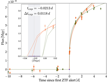
Figure 2. Early light-curve fits used to determine the explosion date for SN 2018dfc. Power-law fits to the observations during the first 2 or 5 days are shown in both the g, (green points) and r, (red points) bands. The mean and standard deviation of the fits (inset) are adopted as the explosion time and the error. The time origin is defined as the time of the first alert from ZTF.
Download figure:
Standard image High-resolution image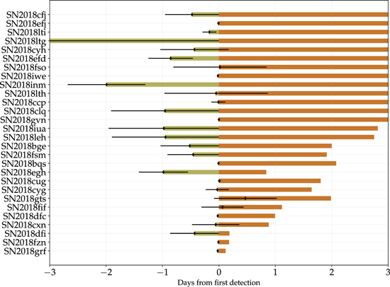
Figure 3. A graphic summary of the sample timeline, from the estimated explosion date (green) to the time of the first spectrum (red). The x-axis origin ("0" time) corresponds to the first photometric detection of each candidate. The black diamonds correspond to the estimated explosion time. SN 2018ltg was included in the sample of RI SNe II since its non-detection limit from the Marshal alert system was <2.5 days even though the explosion time estimation from the forced photometry light curve puts the last limit more than three days earlier.
Download figure:
Standard image High-resolution image3.2. Peak Magnitude
Following Khazov et al. (2016), we also tested whether events showing flash features are, on average, more luminous. As shown in Table 2, the relevant events to consider are only those with relatively early spectra. We therefore compute the peak magnitude of all seventeen events with a first spectrum obtained within seven days from explosion. In the literature, we rarely found flash ionization features which last more than a week from the EED. A first spectrum obtained a week after the EED could miss potential flash features. We hence chose the seven-day sub-sample in order to increase our pool of objects for this analysis while maintaining a realistic estimation of the percentage of flash ionization events. We used the forced photometry light curves to evaluate the peak magnitude. We fitted a polynomial of order 3 to the flux measurements over several intervals of time. The lower bound of these fits is within the first few days from explosion time and the upper bound between 10 and 40 days after the estimated explosion time (Figure 4). We varied randomly the lower and upper boundaries and repeated the fit a hundred times. We adopted the mean and standard deviation of peak times obtained as the peak date and its error (vertical gray band in Figure 4) and took the mean and standard deviation of the flux value as the peak flux and error (horizontal gray band in Figure 4). The absolute peak magnitude is computed as:

with dm, the distance modulus and Aλ the milky way extinction. We report these values for each event in each available band in Table 4. We obtained the dm using the python package astropy.cosmology (Price-Whelan et al. 2018) with the Planck18 cosmology. The extinction was calculated using the packages sdfmap 34 to estimate E(B − V) and extinction (Barbary 2016) for Aλ . We assumed RV = 3.1 and the Cardelli et al. (1989) extinction law. The errors on the absolute magnitude were calculated with:

with δ
mpeak, the error from the fit. We assume here that the error on the distance modulus is linear with the redshift, hence:  . Redshift errors were gathered from NED, when available. We estimated the redshift of the remaining supernovae by fitting a Gaussian shaped line to narrow Hα
emission line. We favored spectra contaminated by host galaxy lines. We used the package minuit (Dembinski et al. 2020) to fit the Hα
line. We remark that the redshift errors are bigger whenever we were using low-resolution SEDm spectra.
. Redshift errors were gathered from NED, when available. We estimated the redshift of the remaining supernovae by fitting a Gaussian shaped line to narrow Hα
emission line. We favored spectra contaminated by host galaxy lines. We used the package minuit (Dembinski et al. 2020) to fit the Hα
line. We remark that the redshift errors are bigger whenever we were using low-resolution SEDm spectra.

Figure 4. Example of the peak estimation in the red band for SN2018dfc. The different curves correspond to a polynomial of order 3 fitted over the time intervals noted in the legend. The cross corresponds to the peak date and flux estimated from the mean of all the values obtained, and the gray bands note the estimated errors, see text for details.
Download figure:
Standard image High-resolution imageTable 4. Peak Absolute Magnitudes of the 17 Objects Within the 7 day Spectroscopic Sub-sample
| IAU Name | Filter | z ± δz | dm | mpeak ± δ mpeak | dpeak ± δ dpeak | Extinction | Mpeak ± δ Mpeak |
|---|---|---|---|---|---|---|---|
| (AB mag) | (AB mag) | (days) a | (AB mag) | (AB mag) | |||
| SN2018bge | r | 0.02389 ± 0.00011 | 35.159 | 17.823 ± 0.005 | 19.039 ± 0.837 | 0.044 | −17.380 ± 0.162 |
| g | 17.900 ± 0.003 | 10.310 ± 0.859 | 0.062 | −17.321 ± 0.162 | |||
| SN2018bqs | r | 0.04730 ± 0.00060 b | 36.675 | 18.776 ± 0.015 | 8.099 ± 0.295 | 0.017 | −17.916 ± 0.499 |
| g | 18.759 ± 0.021 | 6.146 ± 0.308 | 0.024 | −17.941 ± 0.499 | |||
| SN2018clq | g | 0.04509 ± 0.00001 | 36.572 | 18.081 ± 0.004 | 5.158 ± 0.961 | 0.250 | −18.742 ± 0.009 |
| r | 18.118 ± 0.022 | 3.541 ± 1.005 | 0.176 | −18.631 ± 0.023 | |||
| SN2018cxn | r | 0.04070 ± 0.00012 | 36.343 | 18.860 ± 0.006 | 15.844 ± 0.795 | 0.040 | −17.523 ± 0.107 |
| g | 18.864 ± 0.012 | 10.414 ± 0.686 | 0.057 | −17.536 ± 0.108 | |||
| SN2018cug | g | 0.05000 ± 0.00373 c | 36.804 | 18.580 ± 0.006 | 8.560 ± 0.467 | 0.129 | −18.352 ± 2.746 |
| r | 18.592 ± 0.009 | 12.140 ± 0.488 | 0.091 | −18.303 ± 2.746 | |||
| SN2018cyg | r | 0.01127 ± 0.00001 | 33.507 | 18.176 ± 0.009 | 16.008 ± 0.814 | 0.041 | −15.372 ± 0.031 |
| g | 19.171 ± 0.007 | 11.240 ± 0.355 | 0.059 | −14.394 ± 0.031 | |||
| SN2018dfc | r | 0.03653 ± 0.00009 | 36.102 | 17.603 ± 0.005 | 10.663 ± 0.168 | 0.193 | −18.692 ± 0.089 |
| g | 17.555 ± 0.007 | 7.553 ± 0.368 | 0.274 | −18.821 ± 0.089 | |||
| SN2018dfi | g | 0.03130 ± 0.00016 | 35.758 | 17.987 ± 0.002 | 1.803 ± 0.432 | 0.070 | −17.841 ± 0.183 |
| r | 18.161 ± 0.037 | 3.482 ± 2.804 | 0.049 | −17.646 ± 0.187 | |||
| SN2018egh | r | 0.03773 ± 0.00010 | 36.174 | 19.384 ± 0.001 | 17.785 ± 0.911 | 0.070 | −16.860 ± 0.096 |
| g | 19.548 ± 0.007 | 14.102 ± 1.349 | 0.100 | −16.725 ± 0.096 | |||
| SN2018fzn | g | 0.03740 ± 0.00036 b | 36.154 | 18.846 ± 0.019 | 19.266 ± 0.984 | 0.269 | −17.577 ± 0.350 |
| r | 18.505 ± 0.009 | 22.641 ± 0.549 | 0.189 | −17.838 ± 0.350 | |||
| SN2018fif | g | 0.01719 ± 0.00003 | 34.434 | 17.471 ± 0.011 | 12.400 ± 0.644 | 0.351 | −17.314 ± 0.061 |
| r | 17.227 ± 0.006 | 17.048 ± 0.682 | 0.248 | −17.454 ± 0.060 | |||
| SN2018fsm | g | 0.03500 ± 0.00366 c | 36.006 | 17.939 ± 0.009 | 6.334 ± 0.631 | 0.325 | −18.393 ± 3.765 |
| r | 18.051 ± 0.011 | 9.460 ± 3.238 | 0.229 | −18.184 ± 3.765 | |||
| SN2018gts | g | 0.029600 ± 0.00018 | 35.634 | 18.906 ± 0.009 | 6.248 ± 0.623 | 0.059 | −16.787 ± 0.217 |
| r | 18.315 ± 0.004 | 8.525 ± 0.579 | 0.041 | −17.360 ± 0.217 | |||
| SN2018grf | r | 0.05380 ± 0.00307 c | 36.969 | 18.463 ± 0.006 | 7.438 ± 0.279 | 0.081 | −18.587 ± 2.110 |
| g | 18.406 ± 0.005 | 5.624 ± 0.509 | 0.115 | −18.678 ± 2.110 | |||
| SN2018gvn | g | 0.04330 ± 0.00333 c | 36.481 | 18.359 ± 0.028 | 7.604 ± 1.791 | 0.137 | −18.259 ± 2.806 |
| SN2018iua | r | 0.04150 ± 0.00284 c | 36.386 | 18.943 ± 0.005 | 15.001 ± 1.016 | 0.083 | −17.527 ± 2.490 |
| g | 19.114 ± 0.015 | 4.043 ± 2.824 | 0.118 | −17.391 ± 2.490 | |||
| SN2018leh | g | 0.02390 ± 0.00003 | 35.160 | 17.092 ± 0.005 | 13.735 ± 0.983 | 0.838 | −18.905 ± 0.044 |
| r | 17.156 ± 0.045 | 16.186 ± 1.282 | 0.590 | −18.594 ± 0.063 |
Notes.
a Measured with respect to the EED. b The redshift was measured based on a spectrum from SEDm. c The redshift was measured based on a higher-resolution spectrum (e.g., DBSP and APO, here).A machine-readable version of the table is available.
Download table as: DataTypeset image
3.3. Early Spectroscopy
We sorted the 28 RI SNe in our sample according to the difference between the estimated explosion time and the time of the first spectrum (Table 2, "First spectrum" column; Figure 3). From previous work (Gal-Yam et al. 2014; Khazov et al. 2016; Yaron et al. 2017), we know that flash features are typically present from the time of explosion up to several days later. We, therefore, defined a sub-sample including events with spectra obtained within 2 days from explosion (top of Table 2), which includes about one third of the total sample (ten objects).
Throughout the 2018 campaign, we found that seven infant supernovae of Type II show flash features (Table 2; Figure 5). Two additional infant objects were marked as potential flash events (Figure 8; see below). Four of the seven confirmed flashers had their first spectrum obtained with SEDm.
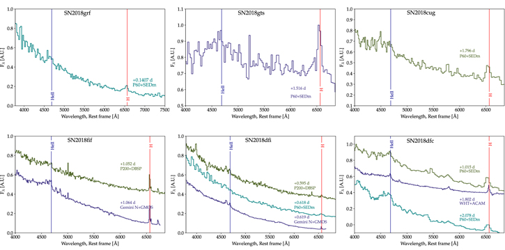
Figure 5. A collection of spectra of six confirmed flashers. The acquisition time of the spectra are given with regard to the estimated explosion date.
Download figure:
Standard image High-resolution imageThe two-day sub-sample includes six events showing flash features, two potential flashers (SN 2018cyg and SN2018egh, Figure 8), and two events which have high signal-to-noise early spectra that show no flash features (Figure 7). One object, SN 2018leh, shows flash features but its first spectrum was obtained >3 days after explosion, see Table 2, Figure 6.
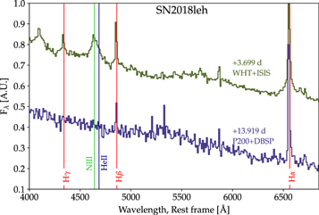
Figure 6. Spectroscopic evolution of SN 2018leh, a Type IIn SN that shows transient He ii emission four days after its estimated explosion time.
Download figure:
Standard image High-resolution image3.3.1. The Flash Events
The identification of flash features in this work is focused on the spectral range surrounding the strong He ii emission line at 4686 Å. This follows previous work (Khazov et al. 2016) and is also supported by theoretical model grids (Boian & Groh 2020) which show that this feature is ubiquitous in early spectra (<2 days). We chose not to use hydrogen lines as a marker for flash features since contribution from host galaxy lines is likely to complicate the analysis.
In previous well-studied cases of events with high-quality early spectra, such as SN 2013fs (Yaron et al. 2017) and SN 2013cu (Gal-Yam et al. 2014), the He ii λ4686 line is very prominent with a profile that is often well described by a narrow core with broad Lorentzian wings, which could be attributed to electron scattering within the CSM (Huang & Chevalier 2018).
As discussed in detail by Soumagnac et al. (2020), while the spectra of such events evolve with time, the strong He ii emission line is replaced by a ledge-shaped feature that is probably composed of blended high-ionization lines of C, N and O. The He ii line and some other lines (e.g., C iii or N iii) are sometimes detected as a narrow emission line on top of the ledge-shaped feature (see Figure 5 and Figure 7 of Soumagnac et al. 2020).
As several of our early spectra were obtained with the low-resolution SEDm instrument (in particular those of SN 2018grf, SN 2018gts, and SN 2018cug), we could not easily differentiate between the various manifestations of the excess emission around 4686 Å. We therefore adopted the detection of excess emission around this wavelength as our criterion for defining an object as having flash features. Analysis of the cases where we have both early SEDm spectra and high spectral resolution data from larger telescopes (e.g., SN 2018dfc), confirm the nature of the emission we see in the SEDm spectra and support our approach (Figure 5).
SN 2018leh is the seventh object which displayed flash features. It does not belong to the sub-sample we considered for this study since its first spectrum was obtained ≈ 3.7 days after the estimated explosion time. This object shows the Balmer emission lines Hα, Hβ and Hγ that persist for an extended period of time, ≈ 10 days. This led us to classify this event as a SN IIn. The first spectrum also shows a strong He ii line, which disappeared about ten days later, see Figure 6. The transient He ii line would technically qualify this event as a member of the flash class. The flash features of this object seem to last longer than the rest of our flasher sample. A discussion of the group of objects displaying long-lived flash features, and their relation to some SNe IIn (e.g., SN 1998S; Lentz et al. 2001, and SN 2018zd; Zhang et al. 2020), is outside the scope of this paper.
3.3.2. The Non-flashers
We defined an event as lacking flash features when we had early, high-quality spectra (i.e., high S/N or higher resolution than SEDm) that did not show any excess emission around He ii 4686 Å. Often, this meant that the spectrum was blue and featureless. Among the ten events included in our 2 day sub-sample, SN 2018fzn was observed shortly after explosion (0.19 day, Table 2) with SEDm. While the resolution was low, the signal-to-noise was sufficient to determine that we could not find any hint of possible excess emission (Figure 7). Based on the few previous events with spectra that were obtained less than two days from EED (in particular SN 2013fs; Yaron et al. 2017), we expected strong emission lines that would be observable with SEDm (see the simulation in Extended Data Figure 2 of Gal-Yam et al. 2014). The first spectrum of SN 2018cxn was obtained with P200/DBSP less than a day past explosion. The higher resolution and the complete absence of He ii emission (Figure 7) imply no flash feature. For both cases, we conclude that there were no indications for a circumstellar shell.

Figure 7. Early spectra of non-flashers SN 2018fzn and SN 2018cxn. These spectra were both obtained within less than a day from the estimated time of explosion. Only a smooth continuum is observed.
Download figure:
Standard image High-resolution image3.3.3. The Dubious Flashers
SN 2018cyg and SN 2018egh both show excess flux around 4686 Å (Figure 8). However, this excess does not resemble the ledge-shaped feature seen, for example, in the spectra of SN 2018fif (Soumagnac et al. 2020), and discussed above. An additional complication is that the spectra of SNe II at the early phase (prior to the appearance of strong and broad hydrogen Balmer lines) sometime show an absorption complex extending between ≈ 4000 and 4500 Å. Such a complex appears in the spectra of both SN 2018cyg and SN 2018egh. It was difficult to determine whether the apparent bump around 4600 Å represents an actual excess, or if it rather was the continuum edge redward of an absorption feature. In addition, even though we secured early, high-resolution spectra for these objects (Table 2), they both lacked a narrow emission component from He ii. The broad features were, however, transient and did not appear at later times. These issues made it difficult to determine if these events displayed flash features.
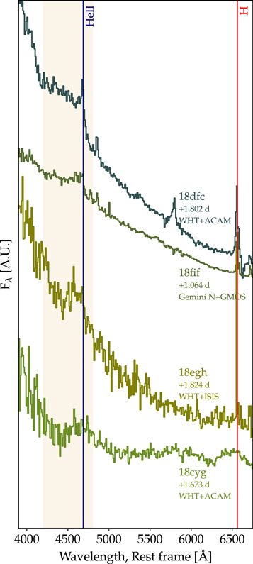
Figure 8. Candidates showing a wide bump-like structure close to the He ii emission line. We highlight in orange the region we searched for excess emission. The spectra of 18cyg and 18egh were both binned to 10Å.
Download figure:
Standard image High-resolution imageAs an additional test of whether these two objects show a flux excess around 4600 Å, we conducted the following test: we constructed model spectra composed of blackbody continua, over which we superposed model Gaussian emission lines whose width was a free parameter (with typical best fits of ≈ 100 km s−1), in those cases (in particular, SN 2018dfc) where such lines were apparent. In addition, we added a broad feature extending between 4200 and 4750 Å, which we defined by fitting a third-order polynomial to the ledge-shaped feature appearing in the SN 2018fif WHT spectrum (Figure 8). The data were fitted using the python package iminuit (Dembinski et al. 2020). We then performed a χ2 test to determine whether the bump feature is significantly detected (in the sense that Δχ2 > 1 between models) by comparing the goodness of fit over the intervals given in Table 5.
Table 5. Results of Test Fits for Models With and Without the Broad Bump Feature
| Name | Spectrum | Lines Fit | χ2/dof | χ2/dof | Fit Interval |
|---|---|---|---|---|---|
| With Bump | Without Bump | (Å) | |||
| SN 2018dfc | P60+SEDm +1.015 days | [He ii, Hβ] | 0.76 | 1.43 | 4000–5300 |
| SN 2018dfc | WHT+ACAM +1.082 days | [He ii, Hβ] | 1.66 | 4.09 | 4000–5300 |
| SN 2018fif | Gemini+GMOS +1.064 days | [He ii, Hβ] | 2.12 | 3.34 | 4000–5000 |
| SN 2018egh | WHT+ISIS +1.824 days | [He ii, Hβ] | 0.87 | 0.91 | 4000–5300 |
| SN 2018egh | WHT+ISIS +1.824 days | No Lines | 0.87 | 0.93 | 4000–5300 |
| SN 2018cyg | WHT+ACAM +1.673 days | No Lines | 0.90 | 0.90 | 4000–5300 |
Download table as: ASCIITypeset image
The results of these model comparisons are reported in Table 5 and Figure 9. As can be seen, the bump was strongly detected in the spectra of SN 2018dfc (and was also recovered for SN 2018fif), but neither for SN 2018cyg nor SN 2018egh. The results did not change if we fitted narrow lines, although no obvious additional lines (e.g., Hγ ) were identified in the spectra. For SN 2018dfc, the bump feature was detected both in the earlier low-resolution SEDm spectrum (at low significance) and clearly in the later high-resolution WHT spectrum. In conclusion, we cannot ascertain that SN 2018cyg and SN 2018egh showed flash features. We report below our results on flash statistics, considering all possible options (i.e., both, one, or neither of these show evidence for CSM).

Figure 9. Fit results with (top panels) and without (bottom panels) the broad feature component for SNe 2018dfc, 2018fif, 2018egh, and 2018cyg (from left to right). No narrow emission lines are seen in the spectra of 2018egh and 2018cyg, and neither provides a significant detection of a bump component.
Download figure:
Standard image High-resolution image4. Discussion and Conclusions
4.1. How Common are Flash Features
Based on our systematic survey of infant SNe II with spectra obtained within two days of discovery, we found that at least 60%, and perhaps as many as 80% of the sample of ten events showed evidence of flash-ionized emission. Taking into account our limited sample size and assuming binomial statistics  , we infer the true fraction of SNe with CSM which manifests as flash features, using a Bayesian model. The true probability p to observe an event with flash features given the observed fraction D is :

Where p is the probability of observing a flash-ionized event (here p ∈ [0; 1] ), D is the observation presented in this paper (i.e.,: 6 out of 10 candidates are showing flash features). The probability of our observation, P(D) can be calculated with the formula of total probability, i.e.,  . We assumed a uniform distribution for the prior π(p), which allowed us to write the posterior function as:
which results in a Beta distribution (see Figure 10). We can put a strict lower limit on the fraction of infant SNe II showing flash features of >30.8% (>23.5%) at the 95% (99%) confidence level (CL). The lower limit rises to 39.1% if either 18cyg or 18egh was a flasher, and to 48.3% if both were, at the 95% CL. This fraction rapidly drops when events with spectra obtained within seven days from explosion are considered (the lower bound drops to 21.5% at the 95% confidence level); presumably the fraction could be even higher for events with even earlier spectra.
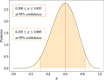
Figure 10. Posterior probability distribution vs. the probability to observe a flash-ionized event. This analysis is based on the sub-sample of infant candidates which had a first spectrum within <2 days from the EED, and considering that 18cyg and 18egh are not flashers. The lower limit is 30.8% (23.5%) at 95%(99%) confidence interval.
Download figure:
Standard image High-resolution imageThese results are broadly consistent with previous work by Khazov et al. (2016), which estimated that 7%–36% of SNe II show flash features in spectra obtained within <2 days from explosion (68% confidence level). It is also consistent with the low observed frequency of flash features among the general population of Type II SNe reported in the literature, as these events very rarely have a spectrum obtained <2 days after explosion. Table 2 shows that the fraction of flash events falls rapidly at ages >2 days. The unique nightly cadence of the ZTF partnership survey enabled us to discover infant SNe routinely, rapidly obtain spectra, and robustly measure the frequency of this phenomenon.
4.2. Possible Biases
Khazov et al. (2016; see their Figure 8) show that Type II SNe showing flash-ionized features tend to be brighter at peak than other events. We cannot confirm that this is also true for our sample. We considered here the sub-sample of infant supernovae whose first spectrum was obtained within less than 7 days from the estimated explosion time. The peak magnitudes were obtained following the method described in Section 3.3.2. Figure 11, top panel, shows the peak magnitudes in both g and r bands for flashers and non-flashers. Flashers appear to be brighter in both bands. However, when one considers SN 2018cyg as a flasher, the average peak magnitude of both groups is inverted, and non-flashers appear brighter than flashers (see Table 6, top section). Since SN 2018cyg is strongly reddened, we repeated this same analysis but with SN 2018cyg being host extinction corrected. To apply the extinction correction, we used the spectrum from 2018 August 4 35 and applied the method described in Poznanski et al. (2012), using the line doublet of sodium. We considered the doublet not to be resolved and apply the following formula:

We estimated the EW of the D1+D2 lines using the built-in tool from WISeREP by measuring it several times. The mean EW is 1.64 Å with an error of 0.17 Å. Following Equation (5), the final peak magnitudes for SN 2018cyg are: Mpeak,r = −18.45 ± 0.50 and Mpeak,g = −18.77 ± 0.80. Table 6 summarizes the different cases: whether SN 2018cyg is a flasher and whether SN 2018cyg was corrected for estimated host extinction. We find that flash events are not inherently brighter than non-flash events.
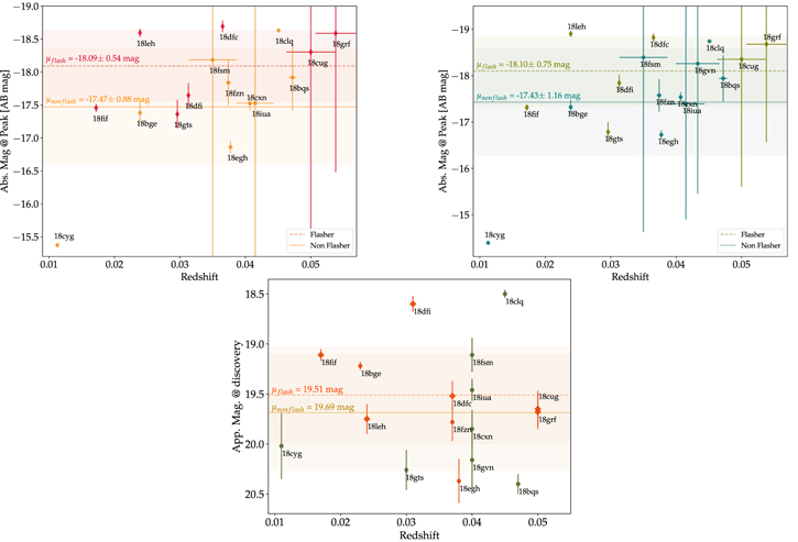
Figure 11. Top: absolute magnitude in r band (left) and g band (right) vs. redshift. Bottom: apparent magnitude at discovery vs. redshift. Color bands represent the error on the mean peak magnitude for both flash and non flash groups. SN 18cyg is host reddened and hence appears very faint, see text.
Download figure:
Standard image High-resolution imageTable 6. Peak Magnitude Comparison Between the Flash Events and the Non Flash Events
| Mpeak,flasher | Mpeak,non flasher | ||
|---|---|---|---|
| 18cyg not corrected for extinction | |||
| r band | 18cyg ⊂ flasher | −17.58 ± 0.96 | −17.76 ± 0.42 |
18cyg  flasher flasher | −17.91 ± 0.48 | −17.46 ± 0.90 | |
| 18cyg corrected for extinction | |||
| 18cyg ⊂ flasher | −17.97 ± 0.48 | −17.76 ± 0.42 | |
18cyg  flasher flasher | −17.91 ± 0.48 | −17.85 ± 0.46 | |
| Mpeak,flasher | Mpeak,non flasher | ||
| 18cyg not corrected for extinction | |||
| g band | 18cyg ⊂ flasher | −17.30 ± 1.31 | −17.64 ± 0.57 |
18cyg  flasher flasher | −17.73 ± 0.71 | −17.31 ± 1.13 | |
| 18cyg corrected for extinction | |||
| 18cyg ⊂ flasher | −17.86 ± 0.75 | −17.64 ± 0.57 | |
18cyg  flasher flasher | −17.76 ± 0.75 | −17.75 ± 0.64 | |
Note. This analysis is performed with the sub-sample which has a first spectrum within less than seven days from the estimated explosion time.
Download table as: ASCIITypeset image
We also inspected in Figure 11, (lower panel) the distribution of apparent magnitudes at discovery for our <7 days sample. As can be seen there, we found that the flash events were not significantly brighter at discovery than other events. Thus neither were more likely to be discovered, nor to be followed-up, as both aspects depend on the apparent magnitude of the object at discovery.
4.3. Implications
We showed here that a significant fraction, and possibly most, Type II SN progenitors, show transient emission lines in their early spectra, which provides evidence that these stars are embedded in a compact distribution of CSM (Yaron et al. 2017). The narrow width of these emission lines indicates a slow expansion speed for the CSM (100–800 km s−1, Boian & Groh 2020), and combined with its compact radial dimension (<1015 cm) we have evidence that the CSM was deposited by the stars within months to a few years prior to its terminal explosion. Assuming these progenitors are mostly red supergiants (RSGs; Smartt 2015), this would suggest that most exploding RSGs experience an enhanced mass loss shortly prior to explosion.
While RSGs certainly lose mass during their final stages of evolution (Smith 2014), such a period of enhanced mass loss shortly (months to a year) prior to explosion is not explained by standard stellar evolution models. Thus, our work indicates that additional physical processes leading to such pre-explosion instabilities (e.g., Arnett & Meakin 2011; Shiode & Quataert 2014) not only exist, but are ubiquitous among massive stars.
As we have shown that most SN II progenitors likely undergo a remarkable evolution shortly prior to explosion, it may be needed to re-examine the stellar models used as initial conditions to explosion simulations. At least some of the effects proposed to explain such pre-explosion mass loss may render the spherical pre-explosion stellar models used in explosion simulations less realistic (Arnett & Meakin 2016). Perhaps our work provides a clue about how to tackle some of the problems encountered in reproducing the observed properties of SN explosions using numerical explosion models.
5. Conclusions
We report the results from the first year (2018) of our systematic survey for infant Type II SNe in the ZTF partnership survey. We collected 28 such objects (at a rate of about one per week) and obtained rapid follow-up spectroscopy within 2 days from explosion for 10 events. Between 6 and 8 of these show evidence for transient emission from a surrounding distribution of CSM. Thus we can place a strict lower limit of >30% (at 95% C.L.) on the fraction of SN II progenitors that explode within compact CSM distributions. This finding is inconsistent with predictions from standard stellar evolution models. It suggests that additional physics is required to explain the final stages (∼1 yr prior to explosion) of massive star evolution. The structural changes that may accompany such final episodes of intense mass loss can modify the stellar structure prior to explosion and may require adjusting the initial conditions assumed for core-collapse SN explosion simulations, and may thus shed light on the yet unsolved question of how massive stars end their lives in supernova explosions.
AGY's research is supported by the EU via ERC grant No. 725161, the ISF GW excellence center, an IMOS space infrastructure grant and BSF/Transformative, Minerva and GIF grants, as well as The Benoziyo Endowment Fund for the Advancement of Science, the Deloro Institute for Advanced Research in Space and Optics, The Kimmel Center for planetary science, The Veronika A. Rabl Physics Discretionary Fund, Paul and Tina Gardner, Yeda-Sela and the WIS-CIT joint research grant; AGY is the recipient of the Helen and Martin Kimmel Award for Innovative Investigation. The ztfquery code was funded by the European Research Council (ERC) under the European Union's Horizon 2020 research and innovation program (grant agreement No. 759194—USNAC, PI: Rigault). The ZTF forced-photometry service was funded under the Heising-Simons Foundation grant #12540303 (PI: Graham). Based on observations obtained with the Samuel Oschin 48 inch Telescope at the Palomar Observatory as part of the Zwicky Transient Facility project. ZTF is supported by the National Science Foundation under grant No. AST-1440341 and a collaboration including Caltech, IPAC, the Weizmann Institute for Science, the Oskar Klein Center at Stockholm University, the University of Maryland, the University of Washington, Deutsches Elektronen-Synchrotron and Humboldt University, Los Alamos National Laboratories, the TANGO Consortium of Taiwan, the University of Wisconsin at Milwaukee, and Lawrence Berkeley National Laboratories. Operations are conducted by COO, IPAC, and UW. The data presented here were obtained [in part] with ALFOSC, which is provided by the Instituto de Astrofisica de Andalucia (IAA) under a joint agreement with the University of Copenhagen and NOTSA. A.A.M. is funded by the LSST Corporation, the Brinson Foundation, and the Moore Foundation in support of the LSSTC Data Science Fellowship Program; he also receives support as a CIERA Fellow by the CIERA Postdoctoral Fellowship Program (Center for Interdisciplinary Exploration and Research in Astrophysics, Northwestern University). Based on observations obtained at the international Gemini Observatory, a program of NSF's NOIRLab, which is managed by the Association of Universities for Research in Astronomy (AURA) under a cooperative agreement with the National Science Foundation. on behalf of the Gemini Observatory partnership: the National Science Foundation (United States), National Research Council (Canada), Agencia Nacional de Investigación y Desarrollo (Chile), Ministerio de Ciencia, Tecnología e Innovación (Argentina), Ministério da Ciência, Tecnologia, Inovações e Comunicações (Brazil), and Korea Astronomy and Space Science Institute (Republic of Korea). This research has made use of the NASA/IPAC Extragalactic Database (NED), which is funded by the National Aeronautics and Space Administration and operated by the California Institute of Technology. The research leading to these results has received funding from the European Union Seventh Framework Programme (FP7/2013-2016) under grant agreement No. 312430 (OPTICON).
Appendix
A.1. Justification of Candidate Rejection
The full list of candidate infant SNe II returned by ztfquery (see Section 2.2) is given in Table 7. Of the 43 candidates, inspection shows that 15 are spurious, and these have been removed from our sample. We provide some comments on removed objects.
Table 7. Results of the Search for Infant SN II using ZTFquery
| Name | R.A. | Decl. | Redshift | First Detection | First | Real? |
|---|---|---|---|---|---|---|
| Spectrum | ||||||
| (deg) | (deg) | (days) | (days) | |||
| ZTF18aaayemw | 134.8982936 | 45.6116267 | 0.052 (NED; Helou et al. 1991) | 2458156.7621 | 0.024 | ⨯ |
| ZTF18aaccmnh | 194.9769678 | 37.8589965 | 0.035 (NED; Helou et al. 1991) | 2458184.8604 | 0.018 | ⨯ |
| ZTF18aagrded | 209.8414748 | 46.0317554 | 0.047 a | 2458198.8809 | 0.011 | ⨯ |
| ZTF18aahrzrb | 181.397224 | 34.3888035 | 0.040 a | 2458217.7371 | 1.001 | ⨯ |
| ZTF18aainvic | 256.5204624 | 29.6683607 | 0.032 a | 2458218.9088 | 0.019 | ⨯ |
| ZTF18aaogibq | 253.5409858 | 24.721127 | 0.037 (NED; Helou et al. 1991) | 2458231.8783 | 0.020 | ⨯ |
| ZTF18aaqkdwu | 199.7588529 | 45.0263019 | 0.060 (NED; Helou et al. 1991) | 2458243.677 | 0.001 | ⨯ |
| ZTF18aaqkoyr | 166.0666639 | 50.0306275 | 0.023 (NED; Helou et al. 1991) | 2458243.6854 | 1.036 | ✓ |
| ZTF18aarpttw | 247.2599041 | 43.6268239 | 0.047 a | 2458246.822 | 1.001 | ✓ |
| ZTF18aarqxbw | 276.4265403 | 34.6584885 | 0.048 a | 2458246.8404 | 1.878 | ✓ |
| ZTF18aasxvsg | 217.1290246 | 37.0678367 | 0.025 (NED; Helou et al. 1991) | 2458244.8361 | 0.018 | ⨯ |
| ZTF18aatlfus | 257.1764284 | 28.5206128 | 0.045 (NED; Helou et al. 1991) | 2458249.8534 | 1.913 | ✓ |
| ZTF18aavpady | 273.0031098 | 44.3602114 | 0.047 a | 2458257.8452 | 0.870 | ✓ |
| ZTF18aawyjjq | 263.0587448 | 36.0740074 | 0.040 a | 2458263.796 | 0.011 | ✓ |
| ZTF18aayxxew | 197.1395703 | 45.9861525 | 0.061 a | 2458278.7043 | 1.961 | ✓ |
| ZTF18abcezmh | 269.4519011 | 40.0764001 | 0.057 a | 2458288.7881 | 0.874 | ✓ |
| ZTF18abckutn | 237.0269066 | 55.7148077 | 0.040 (NED; Helou et al. 1991) | 2458290.6992 | 0.834 | ✓ |
| ZTF18abcptmt | 267.3298968 | 49.4124315 | 0.050 a | 2458291.7869 | 0.878 | ✓ |
| ZTF18abcqhgr | 254.818188 | 60.4317998 | 0.070 (NED; Helou et al. 1991) | 2458291.8048 | 0.021 | ⨯ |
| ZTF18abdbysy | 233.5352962 | 56.6968517 | 0.011 (NED; Helou et al. 1991) | 2458295.7208 | 0.016 | ✓ |
| ZTF18abddjpt | 278.7048393 | 38.2987246 | 0.070 a | 2458295.7913 | 0.021 | ✓ |
| ZTF18abeajml | 252.0323502 | 24.3041089 | 0.037 (NED; Helou et al. 1991) | 2458303.7989 | 1.002 | ✓ |
| ZTF18abffyqp | 252.7086818 | 45.397907 | 0.031 (NED; Helou et al. 1991) | 2458307.6862 | 0.864 | ✓ |
| ZTF18abgqvwv | 254.3164613 | 31.9632993 | 0.038 (NED; Helou et al. 1991) | 2458313.7295 | 0.891 | ✓ |
| ZTF18abgrbjb | 274.9986631 | 51.7965471 | 0.030 a | 2458313.7492 | 0.032 | ✓ |
| ZTF18abimhfu | 240.1422651 | 31.6429838 | 0.050 a | 2458320.6667 | 0.912 | ✓ |
| ZTF18abojpnr | 297.4871203 | 59.5928266 | 0.037 a | 2458351.7166 | 0.021 | ✓ |
| ZTF18abokyfk | 2.3606444 | 47.3540929 | 0.017 (NED; Helou et al. 1991) | 2458351.8659 | 0.887 | ✓ |
| ZTF18abrlljc | 253.1840255 | 70.0882366 | 0.050 a | 2458359.7 | 0.054 | ✓ |
| ZTF18absldfl | 33.5997507 | 30.811929 | 0.035 a | 2458363.8793 | 0.913 | ✓ |
| ZTF18abufaej | 4.4825733 | 12.0916007 | 0.062 a | 2458368.8738 | 0.036 | ✓ |
| ZTF18abvvmdf | 249.1975409 | 55.7358424 | 0.030 (NED; Helou et al. 1991) | 2458375.7154 | 0.016 | ✓ |
| ZTF18abwlsoi | 261.8976711 | 71.5302584 | 0.054 a | 2458377.6334 | 0.895 | ✓ |
| ZTF18abyvenk | 273.9764532 | 44.6964862 | 0.043 a | 2458385.6212 | 0.858 | ✓ |
| ZTF18acbwvsp | 341.9067649 | 39.8806077 | 0.017 (NED; Helou et al. 1991) | 2458423.6368 | 0.907 | ⨯ |
| ZTF18acecuxq | 68.8323442 | 17.1948085 | 0.026 (NED; Helou et al. 1991) | 2458431.8168 | 1.011 | ⨯ |
| ZTF18acefuhk | 136.7936282 | 43.9207446 | 0.058 (NED; Helou et al. 1991) | 2458426.9469 | 0.951 | ⨯ |
| ZTF18acgvgiq | 204.0157722 | 66.3012068 | 0.010 (NED; Helou et al. 1991) | 2458432.0181 | 1.966 | ⨯ |
| ZTF18achtnvk | 96.1687142 | 46.5039037 | 0.040 a | 2458434.9036 | 0.043 | ✓ |
| ZTF18acploez | 130.03737 | 68.9031912 | 0.042 a | 2458440.9658 | 1.957 | ✓ |
| ZTF18acqxyiq | 149.8258285 | 34.895493 | 0.038 (NED; Helou et al. 1991) | 2458443.9437 | 0.001 | ⨯ |
| ZTF18adbikdz | 252.014493 | 26.2118328 | 0.034 (NED; Helou et al. 1991) | 2458482.0504 | 0.004 | ⨯ |
| ZTF18adbmrug | 61.2637352 | 25.2619198 | 0.024 (NED; Helou et al. 1991) | 2458482.6991 | 1.897 | ✓ |
Notes. 43 candidates were found, of which 15 (∼35%) were spurious, leaving 28 infant SNe II in our sample.
a This work.Download table as: ASCIITypeset image
Early false positives—A group of objects detected right at the start of the survey (during 2018 March until early April) suffered from unreliable photometry, manifest as a mix of detections and non-detections during the same period, and often during the same night. This is likely due to problematic early references. The mix of detections and non-detections created artificial triggers due to a spurious non-detection just prior to the first detection. This group includes ZTF18aaayemw, ZTF18aaccmnh, ZTF18aagrded (which was also detected by ATLAS 3 days prior to the ZTF false non-detection, and reported to the TNS as AT2018ahi), ZTF18aahrzrb, ZTF18aainvic, and ZTF18aaogibq.
ZTF18aaqkdwu—This trigger resulted from a spurious photometry point generated by the pipeline at the location of SN 2019eoe a year prior to the explosion of the actual SN.
ZTF18aasxvsg—Additional analysis recovered several clear detections prior to the spurious non-detection that triggered this event.
ZTF18abcqhgr—This event is likely a real infant SN II, but we could not recover it using the forced photometry pipeline and it was therefore removed from the sample. This object does not have an early spectrum.
ZTF18acbwvsp—This event was detected by SNHunt and reported to the TNS as AT 2018hqm a few days prior to the only ZTF non-detection, indicating it is likely not a RI SN.
ZTF18acecuxq—The early photometry of this event shows a mix of detections and non-detections during the same nights, and was deemed unreliable. A spectrum obtained within a day of the false non-detection (A. Tzanidakis, 2021, in preparation) is that of an old SN II, supporting this conclusion.
ZTF18acgvgiq—This event was detected by ATLAS and reported to the TNS as SN 2018fru more than 2 months prior to the ZTF non-detection, indicating our non-detections preceding the ZTF first detection were spurious.
ZTF18acefuhk—Updated photometry does not recover a non-detection prior to first detection that satisfies our criteria. This object does not have early spectra.
ZTF18acqxyiq—The forced photometry pipeline did not recover the non-detection by the real-time pipeline, leaving the explosion time poorly constrained.
ZTF18adbikdz—This object was detected by Gaia and reported to the TNS as AT2017isr over a month prior to the first detection by ZTF (when it was already declining). Our single non-detection is spurious.
A.2. Forced Photometry Light Curves
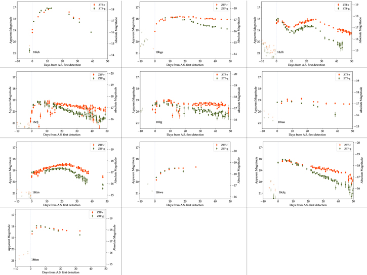
Figure 12. Forced photometry light curves of our Real Infant SN II sample. The gray line represents the first detection from the alert system (i.e., time "0"). Any detection prior to this line was recovered by the forced photometry pipeline. The left y-axis corresponds to the apparent magnitude; the right y-axis to the absolute magnitude. The explosion date of these objects was estimated as the middle date between the last non-detection and the first detection
Download figure:
Standard image High-resolution image
Figure 13. Forced-photometry light curves in both r and g band [continued]. The explosion date of these objects was estimated using the method described in Section 3.3.1.
Download figure:
Standard image High-resolution imageA.3. Classification Spectra of the Real Infant Sample

Figure 14. Classification spectra of the real infant sample. The red vertical line marks the Hα line. See detailed in Table 8.
Download figure:
Standard image High-resolution image
Figure 15. [continued] Classification spectra of the real infant sample.
Download figure:
Standard image High-resolution image
Table 8. List of Photospheric Spectra Corresponding to Figures 14 and 15
| IAU | Estimated | Redshift | Instrument | Time to |
|---|---|---|---|---|
| Name | Explosion Time (JD) | Spectrum (days) | ||
| 18bge | 2458243.1671 | 0.024 | SEDm+P60 | 3.33 |
| 18bqs | 2458246.8133 | 0.047 | DBSP+P200 | 38.69 |
| 18ltg | 2458241.436 | 0.048 | DBSP+P200 | 37.06 |
| 18clq | 2458248.8967 | 0.045 | SEDm+P60 | 7.60 |
| 18cfj | 2458256.4531 | 0.047 | LRIS+Keck I | 55.05 |
| 18ccp | 2458263.7743 | 0.040 | SPRAT+LT | 15.73 |
| 18lth | 2458278.6531 | 0.061 | LRIS+Keck I | 7.85 |
| 18cyh | 2458286.3752 | 0.057 | SEDm+P60 | 16.12 |
| 18cxn | 2458289.8074 | 0.041 | DBSP+P200 | 17.69 |
| 18cug | 2458290.916 | 0.050 | SEDm+P60 | 24.58 |
| 18cyg | 2458294.7273 | 0.011 | DBSP+P200 | 39.77 |
| 18lti | 2458294.6217 | 0.070 | SEDm+P60 | 39.88 |
| 18dfc | 2458303.7777 | 0.037 | SEDm+P60 | 27.72 |
| 18dfi | 2458307.254 | 0.031 | SEDm+P60 | 27.25 |
| 18egh | 2458312.7454 | 0.038 | DBSP+P200 | 38.75 |
| 18efd | 2458312.8922 | 0.030 | DBSP+P200 | 21.61 |
| 18efj | 2458320.6574 | 0.050 | SEDm+P60 | 41.84 |
| 18fzn | 2458351.7068 | 0.037 | SEDm+P60 | 18.79 |
| 18fif | 2458350.9535 | 0.017 | SEDm+P60 | 35.55 |
| 18fso | 2458357.6987 | 0.050 | SEDm+P60 | 13.80 |
| 18fsm | 2458363.4226 | 0.035 | SEDm+P60 | 21.08 |
| 18iwe | 2458368.8561 | 0.062 | SEDm+P60 | 11.64 |
| 18gts | 2458375.1028 | 0.030 | SEDm+P60 | 41.40 |
| 18grf | 2458377.6103 | 0.054 | SEDm+P60 | 65.89 |
| 18gvn | 2458385.6198 | 0.043 | SEDm+P60 | 63.88 |
| 18inm | 2458432.9113 | 0.040 | SEDm+P60 | 15.59 |
| 18iua | 2458439.9877 | 0.042 | SEDm+P60 | 3.51 |
| 18leh | 2458481.7505 | 0.024 | DBSP+P200 | 13.75 |
Download table as: ASCIITypeset image
Footnotes
- 24
Between 2018 March and December.
- 25
- 26
Program IDs OPT/2017B/053, OPT/2018B/011, OPT/2019A/024, PI Gal-Yam.
- 27
IRAF is distributed by the National Optical Astronomy Observatories, which are operated by the Association of Universities for Research in Astronomy, Inc., under cooperative agreement with the National Science Foundation.
- 28
- 29
A parameter calculated by the pipeline that measures the pixel noise in each science image.
- 30
infobitssci is a quality assessment parameter on the processing summary.
- 31
ZTF18aarqxbw, ZTF18aavpady, ZTF18aawyjjq, ZTF18abcezmh, ZTF18abckutn, ZTF18abcptmt, ZTF18abdbysy, ZTF18abddjpt, ZTF18abokyfk, ZTF18abrlljc, ZTF18abvvmdf.
- 32
The light curves presented in this table are not corrected for MW extinction nor for redshift. The absolute magnitude is calculated using the package Distance from astropy (Price-Whelan et al. 2018).
- 33
Each fit is weighted according to the value of the fit on the estimated explosion time.
- 34
- 35
See on WISeREP: https://wiserep.weizmann.ac.il/object/698.