


Abstract
Streamers and pseudostreamers structure the corona at the largest scales, as seen in both eclipse and coronagraph white-light images. Their inverted-goblet appearance encloses broad coronal loops at the Sun and tapers to a narrow radial stalk away from the star. The streamer associated with the global solar dipole magnetic field is long-lived, predominantly contains a single arcade of nested loops within it, and separates opposite-polarity interplanetary magnetic fields with the heliospheric current sheet (HCS) anchored at its apex. Pseudostreamers, on the other hand, are transient, enclose double arcades of nested loops, and separate like-polarity fields with a dense plasma sheet. We use numerical magnetohydrodynamic simulations to calculate, for the first time, the formation of pseudostreamers in response to photospheric magnetic-field evolution. Convective transport of a minority-polarity flux concentration, initially positioned under one side of a streamer, through the streamer boundary into the adjacent preexisting coronal hole forms the pseudostreamer. Interchange magnetic reconnection at the overlying coronal null point(s) governs the development of the pseudostreamer above—and of a new satellite coronal hole behind—the moving minority polarity. The reconnection dynamics liberate coronal-loop plasma that can escape into the heliosphere along so-called separatrix-web ("S-Web") arcs, which reach far from the HCS and the solar equatorial plane, and can explain the origin of high-latitude slow solar wind. We describe the implications of our results for in situ and remote-sensing observations of the corona and heliosphere as obtained, most recently, by Parker Solar Probe and Solar Orbiter.
Export citation and abstract BibTeX RIS

Original content from this work may be used under the terms of the Creative Commons Attribution 4.0 licence. Any further distribution of this work must maintain attribution to the author(s) and the title of the work, journal citation and DOI.
1. Introduction
Understanding the origins of the solar wind and interplanetary magnetic field, which dictate the composition of our heliosphere, remains one of the most enduring and important problems in solar system science. Decades of space- and ground-based observations have clearly established that the structure and dynamics of the wind and heliosphere are determined by the solar magnetic field, which directly couples the solar surface, through the chromosphere and transition region, to the corona and heliosphere. At the photosphere, the field is observed to form a complex and ever-changing pattern of positive and negative magnetic polarities, and while the coronal magnetic field is more difficult to measure, its structure can be inferred from extrapolations and observations of bright coronal threads. These show that in many locations, the magnetic field lines arc up into the solar atmosphere, connecting two opposite polarities as "closed" loops, while in other parts of the atmosphere, the dynamic pressure of the solar wind stretches the magnetic field out to great distances, forming "open" magnetic flux tubes, where coronal plasma can escape freely into the heliosphere. Such open regions are generally accepted to be coincident with the observed "coronal holes" in X-ray and EUV observations, indicating that the heating in these regions is balanced primarily by the solar-wind enthalpy flux rather than the coronal/transition-region radiation flux, as in closed regions (for a review, see Mackay & Yeates 2012). The structure of the heliosphere, therefore, is largely determined by the distribution of magnetic flux at the solar surface.
The lowest-order contribution to the magnetic field comes from the Sun's global dipole moment. Together with the requirement that the interplanetary field be quasi-radial, a purely dipolar photospheric flux distribution exhibits open magnetic field lines in the polar regions (two polar coronal holes) with an equatorial band of closed magnetic flux that sits beneath the global helmet streamer (HS). The surface that encloses the HS forms the boundary between open- and closed-field regions. Observationally, as in eclipse images, the HS appears as an archlike "arcade" structure sitting on the solar limb, with a bright stalk extending radially from its apex outward into the heliosphere (see Figure 1). This bright stalk contains the heliospheric current sheet (HCS) that separates open-field regions of opposite magnetic polarity. Since plasma is constrained to move with the magnetic field, any dense closed-field material that is somehow released onto the open field at the HS boundary ultimately moves outward within or near the HCS. This partly explains the observed brightness of heliospheric streamer stalks, although questions remain concerning the properties of the plasma near the HCS.
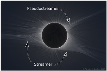
Figure 1. Visible-light image of 2017 August 21 total solar eclipse, copyright 2017 by Nicolas Lefaudeux (https://hdr-astrophotography.com/solar-eclipses/). Image borrowed by permission, with annotations added for clarity. The streamer is visible on the east and southwest limbs. A pseudostreamer is also visible on the northwest limb, exhibiting a bright stalk above twin arcades.
Download figure:
Standard image High-resolution imageSince the photospheric flux distribution nearly always exhibits a global dipole component—except possibly for rare occasions near solar maximum when the quadrupolar component dominates (Wang 2014)—a single HS is typically visible in the corona producing a single current sheet in the heliosphere (the HCS). This observation is also consistent with interplanetary measurements, which typically show a rotational discontinuity that occurs across a single HCS (Owens & Forsyth 2013). Additional magnetic complexity corresponds to higher-order terms in the multipole moment of the photospheric flux distribution, as would be needed, for example, to describe a bipolar active region at high latitude. Such structures create small "parasitic-polarity" domains within the otherwise unipolar hemispheres and add substantial topological richness to the coronal field.
If a parasitic-polarity region occurs inside a coronal hole or inside the HS boundary very near a coronal hole, it creates a new boundary between open and closed flux or strongly distorts the existing one. This invariably adds new bright coronal rays that extend out into the heliosphere, similar to but distinct from the streamer stalks. These structures were first observed decades ago by space-borne coronagraphs and labeled "plasma sheets" by Hundhausen (1972). Their distinguishing feature is that they are not located along the boundary of opposite-polarity domains and need not, therefore, support a current sheet. As a result, these structures were later renamed "unipolar streamers" by Zhao & Webb (2003) and, eventually, termed "pseudostreamers" by Wang et al. (2007). The latter term has gained widespread acceptance, so we use it in this paper.
Pseudostreamers—together with streamers and other structures along the boundary of coronal holes—are associated with strong spatial variations in the composition and speed of the solar wind (see, e.g., Owens et al. 2013; Wang & Ko 2019), which has been established through decades of in situ measurements to consist of two distinct types, the so-called "fast" and "slow." The fast wind has speeds around 750 km s−1, is relatively steady, and, at solar minimum, is found at high heliolatitudes over the Sun's rotational/magnetic poles, which are dominated by polar coronal holes during that time. By contrast (again around solar minimum), near the ecliptic plane and the streamer belt, the slow wind speed is found to be highly variable, with an average around 400 km s−1 (e.g., McComas et al. 2000). Closer to solar maximum, the wind streams become much more mixed in their relative locations due to the enormous complexity of the photospheric flux distribution.
While it has been broadly established that the near-steady fast solar wind emanates from within coronal holes, a definitive understanding of the origin of the filamentary and rapidly varying slow solar wind (SSW) remains to be established (for a review, see Abbo et al. 2016). One key difference between the fast and slow wind streams is their distinct plasma composition. In the fast wind, the elemental abundances are found to be independent of the first ionization potential (FIP) and similar to those of the photosphere, while, by contrast, the slow wind exhibits an enhancement of elements with low FIP compared to those with high FIP (von Steiger et al. 2000). This so-called FIP effect means that the slow wind has abundances that are similar to those found in the magnetically closed corona. This suggests that at least some of the material that forms the SSW originates in the closed-field region, which is possible only if plasma is exchanged between open and closed flux domains (Fisk et al. 1998; Antiochos et al. 2011), most likely through the process of "interchange reconnection" (Crooker et al. 2002).
Initially, it was believed that the SSW was associated only with the streamer belt and that pseudostreamers would be sources of fast wind (Wang et al. 2007), but more recent observations have shown that the SSW emanates from near the whole open/closed boundary, including the vicinity of pseudostreamers (Riley & Luhmann 2012; Viall & Vourlidas 2015; Wallace et al. 2020). In fact, one of the most challenging aspects of the SSW from a theoretical viewpoint is its large angular extent, up to 30◦ or more from the HCS (Tokumaru et al. 2010). Furthermore, even during solar minimum, the SSW constitutes a substantial fraction of the solar wind, ∼30% or more. This observation led directly to the so-called separatrix-web (S-Web) model (Antiochos et al. 2011), which asserts that the SSW originates from a complex network of separatrix and quasi-separatrix arcs in the heliosphere, all mapping down to pseudostreamers in the corona, most of them having topology that is analogous to the structures that we model below.
As discussed above, the streamer belt and associated HCS are always present, and their evolution is fairly well understood (Wang et al. 2000). The pseudostreamers and S-Web arcs, on the other hand, appear and disappear in response to the evolution of the photospheric flux. Since a substantial portion of the SSW is thought to be associated with pseudostreamers, the dynamics of pseudostreamer formation and disintegration are vital to understanding the SSW and modeling the space weather that propagates through this wind. This is the motivation for our paper.
We present below the first detailed 3D numerical simulations of the formation of a pseudostreamer and discuss the implications of the simulations for the origins of the slow wind. We also predict observables for both in situ and remote-sensing instruments. In the following section, we review some of the previous work and background theory on magnetic topology and reconnection. In Sections 3 and 4, we describe our simulation design and results, and we finish with a discussion and conclusions.
2. Theory and Models
2.1. The Open/Closed Boundary and the S-Web
In order to understand the implications of interchange reconnection for the SSW, we must consider the magnetic topology of the flux surfaces that partition open and closed magnetic domains in the corona. By definition, open and closed magnetic flux domains are bounded by separatrix surfaces, which are generally associated with magnetic nulls (isolated points in space where the field strength is identically zero) or, less commonly, bald patches (curves on the photosphere at which the magnetic field lines are tangent). The separatrix surface that defines the HS boundary is a special case, and its topological description depends on the formulation of the heliospheric magnetic field 6 ; however, in potential-field source-surface (PFSS) models, the apex of the HS occurs along a null curve at the source surface, and this defines the separatrix surface of the HS boundary, with more complex models supporting logical extensions of this idea. Under ideal evolution, the plasma is constrained to move with the magnetic field by the so-called "frozen-in condition," which dictates that the field-line velocity and fluid velocity are equivalent, so magnetic flux domains naturally discretize the plasma containment. In order to violate this equivalence on scales larger than the ion gyroradius—as is necessary for the substantial release of plasma from the closed corona into open-field regions—the magnetic field must reconnect.
It is well established that in three dimensions, magnetic reconnection may occur wherever there is a sufficiently large electric current parallel to the magnetic field (Schindler et al. 1988). Moreover, null points and separatrix surfaces (together with quasi-separatrix layers, QSLs) are preferential locations for current accumulation (for a review, see Pontin 2012), meaning that interchange reconnection is expected to be ubiquitous. Antiochos et al. (2011) realized that interchange reconnection might also occur in locations where groupings of parasitic polarity distort the HS separatrix surface in such a way as to come close to itself at some location, forming a narrow corridor of open magnetic flux at the photosphere. Moreover, they demonstrated that the collection of QSLs thus formed, together with the null-point and bald-patch separatrix surfaces in the corona, fills out an equatorial band in coronal field extrapolations that is consistent with the observed latitudinal extent of the SSW. They termed this collection of QSLs and separatrix surfaces the "S-Web."
2.2. Static Models of S-Web Structures
Given complete knowledge of the magnetic field, identification of structures within the S-Web depends on the characterization of the field-line mapping. One approach is to construct the perpendicular magnetic squashing factor, Q⊥ (see, e.g., Titov 2007; Pariat & Démoulin 2012), which can be interpreted as a measure of the deformation of a flux tube between its two conjugate footpoints. At a separatrix surface, where the mapping is discontinuous, Q⊥ attains infinite measure, while in a hyperbolic flux tube or QSL, Q⊥ is typically large but finite. In this framework the S-Web is then a collection of connected subvolumes in which the magnetic squashing factor, Q⊥, is large or (formally) infinite. As mentioned above, the key point of the S-Web model is that these features indicate the locations in the heliosphere where magnetic field lines connect or pass very near to a boundary between open and closed magnetic flux in the inner corona. Consequently, the S-Web indicates the open field lines onto which interchange reconnection is likely to release closed-field plasma, which can then expand into the heliosphere to form the SSW.
Given the importance of the S-Web for understanding the origins of the SSW, a number of questions immediately arise as to exactly what structures it corresponds to back in the corona and how these form. In all cases considered to date, the existence of an S-Web arc requires the presence of parasitic-polarity regions on the photosphere. In the case considered by Antiochos et al. (2011), the S-Web arc is due to a narrow corridor of open flux that connects two coronal holes. These authors started with a polar coronal hole with a large equatorial extension, a so-called elephant trunk, which is frequently seen during the late phase of the solar cycle (Zirker 1977). Parasitic-polarity regions are then placed on either side of the trunk, between which it is narrowed. The resulting open-field structure is that of a large polar hole connected to a smaller equatorial hole by a narrow corridor of open flux. In the heliosphere, the corridor maps to an S-Web arc that, together with the HCS, forms a closed curve. This curve bounds the open flux originating in the equatorial hole and separates it from that originating in the main polar hole. The critically important features of this topology are that the arc persists irrespective of the width of the corridor, even if singular, and that the angular extent of the arc depends only on the ratio of the fluxes in the equatorial versus polar coronal holes. If this ratio is large, the arc extends far from the HCS, implying that the SSW can occur in the heliosphere far from the HCS, even though it is released by interchange reconnection at the coronal-hole boundary.
Titov et al. (2011) developed an analytical model for the case of an S-Web arc formed by a separatrix surface. Again, they started with an elephant-trunk coronal-hole pattern and then introduced a large, elongated parasitic-polarity region with multiple null points. The parasitic region was positioned so as to cut across the trunk, narrowing it and dividing the unipolar open-field region into two parts. By continuous variation of their model field parameters, they obtained a set of adjacent equilibria with similar morphology but distinctly different topologies. In part of the parameter space, the parasitic polarity created a narrow open-field corridor connecting the main polar coronal hole with a smaller equatorial one, analogous to the configuration in Antiochos et al. (2011). However, as the parasitic region was located further across the trunk, the corridor narrowed down to having zero width when the HS separatrix curve and the separatrix curve defining the flux closing into the parasitic region merged into a single degenerate curve at the photosphere. In the latter case, the satellite coronal hole became "disconnected" from the larger polar coronal hole, despite being embedded in the same unipolar flux domain. The S-Web arc in the heliosphere, however, remained nearly unchanged. This shows that a single arc in the S-Web can support either a QSL corresponding to the open flux from a narrow corridor, a true separatrix surface, or both. In all cases, the presence of a parasitic-polarity region appears to be critical in either narrowing or cutting off the open flux. The resultant structure has all of the properties observed for a pseudostreamer on the limb, apparently separating as it does two open-field regions of the same sign and exhibiting twin magnetic arcades beneath a closed separatrix dome that encloses the parasitic-polarity flux.
More recently, Scott et al. (2018) performed a careful analysis of S-Web arcs in a potential-field extrapolation and reached a similar conclusion regarding the typical composition of the underlying magnetic field. As in other studies, these authors identified the structures within the S-Web by evaluating Q⊥, which they combined with knowledge of the domain connectivity to form slog10 Q⊥ = ±log10 Q⊥. The sign of this measure indicates whether the associated flux is closed (positive) or open (negative), making it especially useful in identifying the boundaries between open and closed domains within the coronal volume. Subsequently, Scott et al. (2019) developed a computational technique for "segmenting" the coronal volume into discrete flux domains bounded by the separatrix surfaces and QSLs of the S-Web and surveyed 11 potential-field extrapolations throughout the solar cycle. They found that the S-Web is composed of an approximately equal combination of structures from each class (separatrix surfaces associated with coronal nulls versus QSLs formed by hyperbolic flux tubes associated with narrow open-field corridors).
2.3. Interchange Reconnection in the S-Web
It should be emphasized that the authors listed above considered only the static topology of the S-Web, not its dynamic formation or evolution. While these studies have advanced our understanding of the underlying magnetic topologies of pseudostreamers and the S-Web, major open questions remain concerning how these structures form and evolve dynamically, the effect of this evolution on the SSW, and the observational signatures. Observationally, the photospheric dynamics giving rise to pseudostreamers seem clear: parasitic polarities typically emerge at mid-latitude as the trailing spots of active regions and then are advected toward the poles by the meridional flow, the so-called "rush to the poles" (Altrock 2014). Nonetheless, it remains to be seen whether the reconnection dynamics and topological evolution of such a configuration can be reconciled with the static equilibria in the aforementioned studies.
Early work related to this topic was undertaken by Edmondson et al. (2010), who studied interchange reconnection in the vicinity of a small bipolar region that was bodily displaced toward the pole. The emphasis of that work was not on pseudostreamers and the S-Web but the implications of the simulations to the Fisk et al. (1998) model for the SSW. Despite this, the result is relevant to the present discussion, as it demonstrates how 3D null-point reconnection (see, e.g., Pontin et al. 2013) enables the emergence of a bipolar flux system from beneath the HS into the polar coronal hole. In particular, as the magnetic field is stressed, the accumulation of current in the non-ideal volume surrounding the null point creates an inflow/outflow paradigm that processes flux from the leading edge of the bipole region, either through or around the null point, to the trailing edge. This erodes the flux between the leading edge of the bipole and the adjacent HS boundary, until eventually the separatrix surface that encloses the bipole becomes cospatial with the HS boundary. At this instant, the outer spine field line of the null passes though the HS boundary and across the HCS, and the entire bipolar flux system instantaneously emerges into the open-field region.
The magnetic configuration in Edmondson et al. (2010) is highly symmetric, with a single null and spine line. Consequently, the system is more applicable to a coronal-hole jet or ray, rather than a large pseudostreamer with a bright stalk. By comparison, configurations with less symmetry may exhibit more nuanced reconnection dynamics owing to their additional topological complexity. When three null points are connected in series along separator lines—as in the TN system investigated below—the footpoints of the two outer spines are connected by the footprint of the fan surface of the central null. Reconnection in the vicinity of the dome can occur in the vicinity of one or more of the nulls or along one or both of the separators.
These considerations of magnetic topology and reconnection are important to our understanding of plasma exchange between open and closed magnetic domains, provided that they can be validated under non-ideal conditions. The above discussion assumes that the topology of the bipolar flux system is stable in time, and only its location relative to the HS changes; however, it remains to be seen whether this assumption is valid for dynamically evolving fields. The goal of this paper is to simulate the evolution of bipolar flux systems adjacent to the HS boundary—with a focus on systems supporting more than one coronal null point—and the subsequent formation of a pseudostreamer following their emergence across the HS boundary.
3. Simulation Design and Methods
In this work, we calculate the dynamics of a bipolar flux system with multiple null points in which the overlying separatrix dome is composed of multiple fan surfaces, each emanating from a different null. We consider two cases resulting from qualitatively similar flux distributions: one with three nulls connected by separator lines and another with only a single null for comparison. The magnetic field is constructed in the simplest configuration that exhibits the needed topological complexity while minimizing elements that complicate the analysis.
We model the background coronal magnetic field ( B ) between the solar surface (R⊙) and the source surface (Rss) with a PFSS model, in which B is prescribed to be purely radial at the source-surface boundary, which we place at Rss = 3 R⊙. In addition to this background dipole field, we include two additional dipoles below the photosphere (and two corresponding mirror dipoles beyond the source surface) that create the requisite bipolar magnetic-field distribution at the photospheric boundary. The dipole locations (listed in Table 1) are set so that the parasitic-polarity region is elongated along the heliocentric east–west direction, with a slight inclination from southwest to northeast to prevent the configuration from being perfectly symmetrical. This elongation is consistent with the observed tendency of polarities to be stretched by differential rotation.
Table 1. Details of Source Magnetic Dipoles
| B0 [G] | d0 [R⊙] | r [R⊙] | ζ [deg] | η [deg] | |
| SN | |||||
| −66.0 | 0.1 | 0.9 | −3.6° | +31.0° | |
| +2444.4 | 0.1 | 10. | −3.6° | +31.0° | |
| −66.0 | 0.1 | 0.9 | +3.6° | +29.7° | |
| +2444.4 | 0.1 | 10. | +3.6° | +29.7° | |
| TN | |||||
| −66.0 | 0.1 | 0.9 | −7.2° | +32.4° | |
| +2444.4 | 0.1 | 10. | −7.2° | +32.4° | |
| −66.0 | 0.1 | 0.9 | +7.2° | +29.7° | |
| +2444.4 | 0.1 | 10. | +7.2° | +29.7° | |
Note. Dipole locations are given in simulation latitude (ζ) and longitude (η), which are rotated 90° with respect to heliocentric angular coordinates. Each dipole moment is set so that the peak field strength B0 occurs at a normalized distance d0 from the dipole center along the dipole axis. All dipoles are oriented along simulation longitude ( ).
).
Download table as: ASCIITypeset image
The inclination of the parasitic-polarity region and its position relative to the global field geometry in both cases is shown by the black polarity inversion lines (PILs) in Figure 2. Initially, the separatrix dome that encloses the parasitic polarity is entirely embedded in the flux beneath the global-scale dipolar HS in each case, which bulges to the north to accommodate the inclusion of this additional flux (Figure 2, middle and bottom panels). Because the open/closed boundary is nowhere folded back on itself (unlike the construction in Antiochos et al. 2011), the presence of this bipolar region beneath the HS has little impact on the flux within the polar coronal hole. Consequently, in the initial condition, the S-Web consists only of the HCS, and no pseudostreamer is initially present in the corona.

Figure 2. Comparison of magnetic configuration between SN (left) and TN (right) cases. The black curves on the photosphere indicate the polarity inversion lines, which enclose the parasitic-polarity flux beneath the separatrix domes. Color maps indicate the radial flux distribution (top) and squashing factor (slog10 Q⊥; middle and bottom). Field lines traced in yellow, white, and green emanate from the various null points. In panels (c)–(f), the location of the open/closed boundary is shown by the abrupt transition between blue (open) and red (closed) regions.
Download figure:
Standard image High-resolution imageThe two cases considered are hereafter referred to as the SN and TN configurations (exhibiting a single null or triple nulls, respectively), which differ only by a slight change in the separation of their source dipoles. In the first case, the dipoles are positioned close together to form a compact flux distribution with a single local maximum in the parasitic-polarity flux. The dome-shaped separatrix surface (separatrix dome) that encloses the bipolar flux system is formed entirely by the separatrix surface of a single null, which is positioned at about 0.12 R⊙ above the photosphere. This simplest configuration is qualitatively very similar to that studied by Edmondson et al. (2010). In the second case, the dipoles are placed sufficiently far apart to create a pair of local maxima in the parasitic-polarity flux. This results in a system of three coronal null points positioned immediately above the parasitic-polarity region at heights between 0.07 and 0.09 R⊙. The nulls are connected by two separator field lines that run nearly parallel to the long axis of the parasitic-polarity region, and the separatrix surfaces from the outer two nulls together form a single separatrix dome that encloses all of the flux from the bipolar region.
The relative similarities and topological distinctions between the SN and TN configurations can be seen in Figure 2, which shows the magnetic flux distributions, the composition of the separatrix domes, and their proximity to the open/closed boundary. The two distinct "lobes" of the TN separatrix dome indicate field lines that map to the spines of the left and right nulls (NL and NR ), which in turn bound the fan surface of the central null (NC ). It is noteworthy that the SN arrangement is actually a special limiting case of the TN arrangement; if any two (or all three) of these nulls become cospatial, the TN case collapses to the simpler SN case. Apart from these distinct topologies, all other aspects of the simulation design are identical between the two cases.
We solve the nonlinear ideal magnetohydrodynamics equations using the Adaptively Refined MHD Solver (ARMS; DeVore & Antiochos 2008), in which the minimal residual numerical diffusion at steep gradients introduces non-ideal effects similar to those resulting from electrical resistivity in resistive models. For simplicity, the plasma is assumed to evolve isothermally at a fixed temperature of T = 2 × 10⁶ K. The gravitational acceleration scales inversely with the square of the radius and is set to g = −2.75 × 104 cm s−1 at the spherical solar surface of radius R⊙ = 7 × 1010 cm. The pressure at the surface is set to p⊙ = 5 × 10⁻² erg cm−3, which fixes the density at that height given the uniform constant temperature T. The pressure and density are then set throughout the rest of the volume to be consistent with hydrostatic equilibrium. The sound speed is constant at cs
≈ 130 km s−1 throughout the volume, while the Alfvén speed varies with the local magnetic-field strength and density. An estimate of the global average Alfvén speed is found by comparing the integrated total magnetic energy (Em
) and total mass (M). This has a value of  for both the SN and TN configurations.
We use a spherical coordinate system with a baseline grid that is 32 × 96 × 192 in log-radius ( ), latitude (ζ), and longitude (η), spanning a domain that extends from r ∈ [R⊙, 3 R⊙], ζ ∈ [−78.75°, +78.75°], and η ∈ [−180°, +180°]. The coordinate system is oriented so that the coordinate poles (ζ = ±90°) are located on the east and west limbs, while the magnetic poles are positioned at ζ = 0°, η = ±90°. With this convention, the polar crown regions are spanned by the numerical domain, away from any coordinate singularities. Beyond this baseline grid, we impose an additional four levels of refinement, each of which doubles the resolution along each coordinate, so that the most finely resolved region has a spatial resolution Δ ≈ 3 × 10³ km ≈ 4 × 10⁻³
R⊙. This scale is much smaller than the local scales of either the magnetic field or the driving velocity field, ensuring ideal plasma evolution except in the reconnecting, grid-scale current structures. Hence, the simulations performed here are very highly resolved, except for the current layers that form at the grid scale near the null points and separator lines during the evolution of the system.
), latitude (ζ), and longitude (η), spanning a domain that extends from r ∈ [R⊙, 3 R⊙], ζ ∈ [−78.75°, +78.75°], and η ∈ [−180°, +180°]. The coordinate system is oriented so that the coordinate poles (ζ = ±90°) are located on the east and west limbs, while the magnetic poles are positioned at ζ = 0°, η = ±90°. With this convention, the polar crown regions are spanned by the numerical domain, away from any coordinate singularities. Beyond this baseline grid, we impose an additional four levels of refinement, each of which doubles the resolution along each coordinate, so that the most finely resolved region has a spatial resolution Δ ≈ 3 × 10³ km ≈ 4 × 10⁻³
R⊙. This scale is much smaller than the local scales of either the magnetic field or the driving velocity field, ensuring ideal plasma evolution except in the reconnecting, grid-scale current structures. Hence, the simulations performed here are very highly resolved, except for the current layers that form at the grid scale near the null points and separator lines during the evolution of the system.
As the two systems evolve, each of the embedded regions is driven toward the nearby magnetic pole by a large-scale pattern of circulating flow. The driving flow, illustrated in the left panel of Figure 3 and described in greater detail in the Appendix, is nearly uniform in the vicinity of the bipoles and returns along the east and west limbs. The flow is incompressible (divergence-free) and designed to avoid shear flows along the edges of the pattern, as well as to minimize flux accumulation at the poles. The flow is mirrored in the two magnetic hemispheres to minimize the deformation of the HCS, thereby simplifying the subsequent analysis. The driving flow achieves a maximum speed  , so it is both subsonic and highly sub-Alfvénic, albeit larger than the observed photospheric velocities for computational efficacy. The flow amplitude is initially zero and ramps up sinusoidally over 800 s to full speed, remains at full speed for the next 6400 s, then ramps down sinusoidally back to zero over the final 800 s.
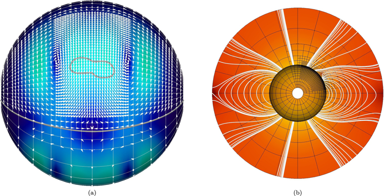
Figure 3. Diagram view of numerical grid in ARMS from two perspectives. Each rectilinear voxel indicates an 8 × 8 × 8 grid block. Left: front view of circulation pattern and angular grid extent with flow speed indicated in blue–green (small–large) color map. Right: side view depicting magnetic configuration and radial grid structure with magnetic-field magnitude depicted in red–yellow (small–large) color map. The region of highest resolution encloses the various magnetic null points and the maximal poleward ( ) flow.
Download figure:
Standard image High-resolution imageWe mandate refinement to the highest resolution in a coronal volume above the photosphere that encloses the null points, with sufficient angular extent to enclose the region of strongest poleward flow. At the bounding surfaces of this high-resolution volume, the refinement gradually steps down one level at a time until it reaches the coarsest resolution set by the baseline grid. This configuration is illustrated by the two coordinate slices in Figure 3, with r = R⊙ on the left and ζ = 0 on the right. The white arrows in the left panel indicate the surface flow velocity, whose magnitude is depicted by the blue–green color map. The red–yellow color map on the right shows the magnitude of the magnetic field, with field lines traced in white.
We employ open boundaries along both angular coordinate directions, ζ and η, and we impose periodic conditions at η = ±180°. Zero-gradient extrapolations are used for all variables at the ζ boundaries except the normal velocity, which is set to zero (reflecting condition). In the radial direction, the logarithmic density and pressure gradients are held fixed at their hydrostatic equilibrium values, and the normal velocity again is set to zero (reflecting) at both boundaries. At the inner boundary, zero-gradient conditions are applied to the transverse velocity components. Except in regions where the analytical flow patterns are imposed, the velocity is prescribed to vanish. The transverse velocity components are set to zero beyond, but not inside, the outer boundary; this allows the field lines to slip along that boundary in response to interior forces and flows. The transverse magnetic-field components are extrapolated assuming zero gradients at the inner boundary; they are set to zero at the outer boundary, consistent with the source-surface condition and the initial magnetic configuration.
We note that the boundary conditions adopted preclude a radial outflow, and detailed calculations of the outflowing solar wind would require a much larger spatial domain encompassing the sonic and Alfvénic points. However, this wind would have no significant impact on the pseudostreamer formation process in the inner corona, where the ambient wind speed is a small fraction of the sound speed. As such, our simulations do not provide direct confirmation of the link between pseudostreamers and slow wind discussed in Section 1. Nevertheless, they reveal several important consequences for understanding the corona and heliosphere, revealing key characteristic dynamics of pseudostreamer formation and the expected observational signatures of this evolution.
In order to analyze our simulation results, we extracted representative snapshots of the magnetic field for the SN and TN configurations, which are indicated with numeric subscripts (e.g., SN3) for the times listed in Table 2. We then applied the QSLsquasher tool developed by Tassev & Savcheva (2017; see also Scott et al. 2017) to create surface and volume renderings of the slog10 Q⊥. We also calculated the locations of the null points in each snapshot using a routine developed by F. Chiti at the University of Dundee and based on the method of Haynes & Parnell (2007). The magnetic field and derived quantities were then visualized using the open-source ParaView application.
Table 2. Integration Time of Selected Simulation Snapshots
| SN1 | 00s |
| SN2 | 46m 40s |
| SN3 | 2h 40m 00s |
| TN1 | 00s |
| TN2 | 22m 40s |
| TN3 | 52m 00s |
| TN4 | 1h 13m 20s |
| TN5 | 2h 18m 40s |
| TN6 | 2h 58m 40s |
Download table as: ASCIITypeset image
4. Simulation Results
The initial evolution of the magnetic field is qualitatively similar in the two configurations. There is a brief relaxation phase while the coronal field settles to a numerical equilibrium and the driving flow builds progressively to its full amplitude (at t = 800 s). During this early evolution, no change to the mapping of open field lines from the source surface down to the photosphere is observed, showing that the evolution is nearly ideal.
Throughout the driving, the apex of the HS is only minimally displaced in latitude due to the symmetry in the driving profile across the equator. The closed boundary condition at the source surface also prevents the apex of the HS from rising through the surface, so the identification of the HS boundary using field lines emanating from the source-surface polarity inversion line is self-consistent throughout the simulations. Toward the east and west limbs, where the flow recirculates toward the equator, the HS pulls away from the source surface as the field lines beneath it contract, eventually pinching off and forming U-loops in the upper corona. However, these occur far from the region of interest and are not relevant to the following discussion.
Once the driving has reached full speed, significant stress accumulates in both the open- and closed-field regions. The boundary conditions on the transverse velocity at the source surface allow the field lines to slip along that surface, so that the open field is generally less stressed than the adjacent closed field. This is to be expected physically; any stress injected on closed field lines simply builds up, whereas on open field lines it can propagate away as Alfvén waves. Also as expected, the stresses tend to accumulate in the weak-field region around the nulls, leading to null collapse and the formation of electric current layers near the null points (Antiochos 1996; Pontin & Craig 2005), as shown in Figure 4. In the figure, the two cases are depicted in snapshots SN2 and TN3 (see Table 2 for timing), which occur after the current layers are fully developed. The formation of these current layers ultimately leads to the onset of reconnection within the non-ideal volumes surrounding the null point(s) and separator lines; the latter are present only in the TN configuration.
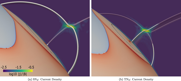
Figure 4. Maps of normalized electric current density (∣ j ∣/∣ B ∣) for states SN2 and TN3 showing the formation of a current layer in the vicinity of NS and NC due to photospheric driving. In both cases, the current is shown in the translucent purple–yellow color scale for a constant-ζ slice through the null system. Here slog10 Q⊥ is shown on the photosphere in the same blue–white–red color scale as in Figure 2, indicating the footprints of the separatrix dome and larger open/closed boundary.
Download figure:
Standard image High-resolution imageA critical property of reconnecting fields is the aspect ratio (a) of the current layer, as this, together with the Lundquist number (S), determines whether reconnection is steady (in a laminar current layer) or bursty (in a fragmented current layer). Wyper & Pontin (2014) found that a 3D plasmoid instability (Loureiro et al. 2007) in a current sheet at a 3D null requires a ≳ 50 and S ≳ 104. From Figure 4, we can estimate a ≤ 10, which, together with the observed steady nature of the reconnection, indicates that for the present simulation parameters, the reconnection is of the Sweet–Parker type. While there is no explicit resistivity, we can estimate a local value of S for the current sheet by noting that in the Sweet–Parker regime, a2 ≃ S, so that S ≤ 100. Thus, we are some way from the onset of nonlinear tearing in the current layer. Were we able to substantially enhance the numerical resolution and reduce the effective dissipation sufficiently, we would expect the reconnection to become bursty (e.g., Ji & Daughton 2011), leading to a substantial increase in the complexity of the dynamics and the resulting magnetic topology (Daughton et al. 2011; Pontin & Wyper 2015). As we will discuss later, the laminar/bursty nature of the interchange reconnection may have important implications for structure within the slow wind.
4.1. Reconnection Dynamics
Following the formation of electric currents near the nulls, the closed flux between the HS boundary and the leading edge of the domes erodes until each eventually emerges, in full or in part, through the flank of the HS. The stages of this emergence are discussed in Section 4.2; here we focus on the reconnection dynamics. Away from the current layers, the plasma evolution is nearly ideal, as the magnetic field lines are locally advected by the flow. We can therefore trace field lines from seed points that are comoving with the fluid in the ideal regions and infer the details of the reconnection by the apparent motion of the conjugate footpoints. In the absence of reconnection, the conjugate footpoints will also be comoving with the fluid. Hence, signatures of reconnection will be apparent in departures of the field-line velocity from the fluid velocity.
The reconnection of flux across one of the null systems is demonstrated for the TN configuration in Figure 5, where we observe changes in connectivity across the separator line NL –NC . In the figure, states TN3 and TN4 are shown with color-coded field lines indicating the domain connectivity. In the upper left panel, the field lines are traced from seed points on the r = R⊙ boundary in the polar coronal hole (blue) and in front of the trailing edge of the bipole domain (red). Closed field lines behind the leading edge of the bipole domain and in the (initially) closed-field region beneath the HS are shown in white. The line elements that define these seed points are shifted between states TN3 and TN4 as if advected by the flow, so that the motion of the footpoints near the leading and trailing edges of the bipole region is consistent with ideal evolution. We observe that in TN4, the transitions between these colored sets of field lines no longer lie on the curve defining the open/closed boundary in the map of slog10 Q⊥. Instead, some of the blue and red field lines have reconnected into the adjacent domains, as shown by the inflow/outflow regions in the lower panels of Figure 5. The disparity between the evolving open/closed boundary and the advected seed points for field lines along this boundary is the hallmark of interchange reconnection across a closed separatrix dome.
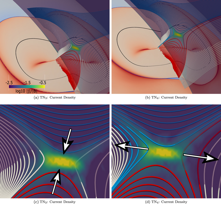
Figure 5. Maps of slog10 Q⊥ on the photosphere in blue–white–red color scale with field lines also traced from the photosphere in the open- and closed-field regions along the leading and trailing edges of the separatrix dome footprint. States TN3 and TN4 are shown in the left and right panels, respectively. In TN3, the color transitions between adjacent field lines reflect the locations of the separatrix dome and fan curtain. In TN4, the locations of the seeds have been shifted to reflect the photospheric flow. The color transitions no longer align with the separatrix surfaces but have moved into the adjacent flux domains, as indicated by the "inflow" and "outflow" regions. Normalized electric current density (∣ j ∣/∣ B ∣) is again depicted in the translucent constant-ζ slice, which is nearly orthogonal to the separator line NL –NC . Field lines appear to darken as they pass through the translucent current density slice, indicating their extension perpendicular to the plane.
Download figure:
Standard image High-resolution imageThe apparent field-line evolution during reconnection depends from which side of the reconnection region the field lines are traced. We can understand how interchange reconnection changes the open flux in the context of the evolving HS boundary by mapping field lines from comoving (stationary, in this case) seeds on the source surface near the apex of the HS, as shown in Figure 6. These field lines are indicative of open heliospheric flux (OHF), which undergoes changes in connectivity in concert with local connectivity changes in the photospheric flux. Once a portion of the fan curtain of NC has emerged into the open field (between TN1 and TN2), OHF from the polar coronal hole begins to reconnect across the separator lines. In Figure 6(a), showing state TN3, a collection of representative field lines that extend northward from the HCS lies entirely in the polar coronal hole on the leading edge of the bipole region. In panel (b), showing state TN4, a subset of these same field lines has reconnected into the satellite coronal hole on the trailing edge of the bipole.
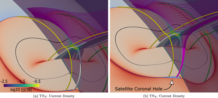
Figure 6. Maps of slog10 Q⊥ on the photosphere in the same blue–white–red color scale with nulls NL and NR and field lines traced from seed points at the source surface. States TN3 and TN4 are shown in the left and right panels, respectively. Normalized electric current density (∣ j ∣/∣ B ∣) is depicted in the translucent slice, which runs orthogonal to the separator line NL –NC .
Download figure:
Standard image High-resolution imageAs this evolution continues, the outer footprint of the fan curtain of NC sweeps out an area of OHF, processing it through the reconnection site. The fan curtain is part of a larger high-Q⊥ volume that forms an arc in the S-Web where it intersects the source surface. That arc, together with the HCS, forms a closed curve containing all of the OHF that is processed through the reconnection region from the poleward to the equatorward sides of the separatrix dome to accumulate in the satellite coronal hole, as shown in Figure 6. Simultaneously, closed flux beneath the trailing edge of the null dome opens through interchange reconnection (Figure 5(b)), so that as the OHF reconnects, it becomes connected to the photospheric flux whose plasma composition is inherited from the closed-field domain. This process is especially relevant to the SSW, as plasma that was previously confined beneath the null dome can now escape along the newly opened field lines into the larger coronal volume and the heliosphere beyond. An analogous process occurs in the SN case, except that there is no central fan curtain and only a single spine field line. Nevertheless, the reconnection occurring within the current sheet around the single null reconnects OHF with previously closed flux on the trailing edge of the separatrix dome.
It is of interest that, for any constant-ζ slice positioned between NL and NR , the evolution of field lines projected onto that slice appears to follow the classic 2D X-point dynamics, though we note that a rapid field-line "flipping" (Priest et al. 2003) occurs out of the plane, as required for 3D reconnection. In static models, nulls NL , NC , and NR can be viewed as resulting from a pitchfork bifurcation of NS , so the eigenvalue of NC along the separator direction is much weaker than that of NS along the same direction. This causes the magnetic-field component along the separator lines to remain weak over a longer distance (from NL to NR ) in the TN case than in the SN case, where it increases quickly away from NS in any direction. Thus, the region of strongly enhanced current (relative to the local field strength) has a longer extent in the east–west direction in the TN case than the SN case.
4.2. Topological Evolution
Both initial states contain appreciable flux between the northernmost edge of the null domes and the flank of the HS, but the processing of flux through the non-ideal regions surrounding the nulls soon brings these topological structures into close proximity. While the reconnection dynamics are similar between the two cases, the progression of topological configurations is significantly more complex in the TN configuration, owing to the increased number of topological elements that comprise the null dome in that case.
Apart from the HS boundary, the SN configuration has only one separatrix fan surface, which forms the entire dome and terminates on a simple closed curve on the photosphere. In contrast, the TN configuration supports three separatrix surfaces that intersect pairwise along separator lines that connect the three nulls; one separator connects NL to NC , and the other connects NC to NR . The separatrix fan surfaces from the most distant nulls (NL and NR ) form two halves of the dome, each terminating on their respective portion of the dome footprint and abutting each other along the spine lines from the central null (NC ). The separatrix fan surface from the central null is orthogonal to the other two and bounded by their respective spine field lines, forming a separatrix curtain (Titov et al. 2011; Platten et al. 2014).
In both configurations, the inner spine lines of the nulls that form the separatrix dome always map to within the parasitic-polarity region, beneath the dome. The outer spine lines adhere to the global field structure, mapping either to the photosphere in the opposite hemisphere or to the outer boundary in the same hemisphere (see Figures 7 and 8). For the fan surfaces that comprise the domes, the field lines all map from their individual photospheric footpoints to the spine line of the associated null (the mapping is degenerate). Thus, if the outer spine line from a given null is open (closed), then all of the field lines of the the associated separatrix fan surface are also open (closed). In the SN case, this implies that the entire separatrix dome must be entirely contained within either the open or closed portion of the larger dipole field, according to the location of the outer spine of NS . In the TN case, on the other hand, the outer spines of NL and NR can be both open, both closed, or one open and one closed, and the two lobes of the associated separatrix dome are similarly situated.
It follows that, in the SN case, as flux reconnects through and around the null NS and the separatrix dome is brought progressively closer to the HS boundary, the ultimate emergence of the null dome into the open field is instantaneous. As soon as this occurs, a continuous corridor of open flux, of initially infinitesimal width, separates the newly emerged separatrix dome from the HS boundary. Following this emergence, as more flux reconnects around the SN dome, the width of the open corridor increases and a small coronal hole forms within the corridor. This process is observed in Figure 7, which depicts the spine and fan surface field lines of NS , as well as the footprints of the various flux domains as the field evolves. Note that in the top row (SN1), the entire null system and its photospheric footprint are within the closed field beneath the HS, but already in SN2 (middle row), the outer spine has transitioned into the open field. The opening of the spine field line coincides with the emergence of the null dome into the open field, as evidenced by the accumulation of open flux along the trailing edge of the dome footprint. Here SN3 (bottom row) is topologically identical to SN2 and illustrates the persistence of this arrangement under continued driving, as well as the accumulated flux in the satellite coronal hole.
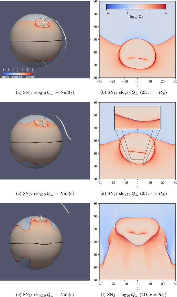
Figure 7. Rendering of slog10 Q⊥ in blue–white–red color scale for the SN configuration in three representative snapshots, SN1 (top), SN2 (middle), and SN3 (bottom). A global 3D rendering is shown in the left column, with representative field lines showing the locations of the spine field line of NS in each snapshot. A zoomed-in version is plotted against unrolled polar (ζ, η) coordinates in the right column. The cutout in the middle right panel shows the presence of reconnected open (blue) flux on the trailing edge of the separatrix dome.
Download figure:
Standard image High-resolution imageIn contrast to the SN case, the TN system emerges into the open-field region in stages, and for a finite but appreciable period of time during this process, the separatrix dome straddles the HS with portions of the central fan curtain in both the open- and closed-field regions. It is also worth noting that the fan surface of NC can cross the HS boundary any even (odd) number of times, provided that the spines of NR and NL lie on the same (opposite) side of the HS boundaries. Therefore, the first field line of the fan curtain to emerge through the HS boundary need not be one of the spines, as evidenced in Figure 8. Note that between TN1 and TN2 (panels (a) and (b)), the connectivity of the spine field lines has not changed; however, a small amount of open flux (depicted in blue) has reconnected across the fan curtain and now connects on the trailing edge of the separatrix dome. Two new intersections between the separatrix curtain and the HS have been formed. The newly reconnected flux is analogous to the satellite coronal hole formed by the SN configuration but differs in that its footprint on the photosphere is surrounded entirely by closed flux beneath the HS; its only connection to the polar coronal hole is along the spine field lines of NC . This is structurally identical to the "detached" coronal holes discussed by Titov et al. (2011) and Scott et al. (2018).
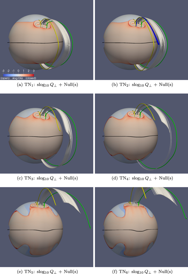
Figure 8. Rendering of slog10 Q⊥ in blue–white–red color scale for the TN configuration in six representative snapshots, TN1–TN6, in panels (a)–(f), respectively. The global 3D rendering is presented with representative field lines indicating the locations of the spines of NL (yellow) and NR (green). White field lines partially represent the location of the fan curtain of NC , which spans a surface that is bounded by the spines of NL and NR . The blue field lines in panel (b) indicate reconnected open flux that has accumulated on the trailing edge of the separatrix dome, behind the fan curtain of NC , prior to the emergence of either spine field line into the open field.
Download figure:
Standard image High-resolution imageThe flux within the detached coronal hole is bounded by the open portion of the fan curtain of NC , which forms an arc on the source surface. This arc, together with a portion of the HCS, forms a closed curve that bounds the open flux within the newly formed coronal hole. The configuration is topologically stable, persisting for an appreciable period of time in our simulation. During this time, flux that reconnects through the null system continues to accumulate in the satellite coronal hole, which remains disconnected until the outer spine of null NL emerges into the open field, as seen in TN3 (panel (c) of Figure 8). Following the emergence of the spine of NL into the open field, the fan curtain of NC straddles the HS boundary and is partly open and partly closed. This state persists for a considerable period of time (spanning TN4), with the particular field line of the separatrix curtain that lies on the HS gradually moving toward the spine of NR . Eventually, the spine of NR opens, just prior to TN5 (panel (e)). The null dome, now completely embedded in the open field, is no longer topologically connected to the HS. This final configuration persists through TN6 and beyond.
This evolution is also evidenced in the photospheric connectivity shown in Figure 9, which displays slices of slog10 Q⊥ corresponding to the same states as in Figure 8. Again, for TN1, the separatrix dome is surrounded entirely by closed flux, while in TN2, a small patch of open flux has accumulated on the trailing edge but does not extend around to connect to the larger polar coronal hole. In TN3, after the emergence of NL , a corridor has formed around the eastern lobe of the null dome so that the satellite coronal hole is now topologically connected to the open flux of the polar region. The coronal hole continues to grow (as seen in TN4), but no topological change is apparent until NR emerges into the open field, evidenced by the narrow corridor of open flux around the western lobe of the null dome in TN5. The satellite coronal hole continues to accumulate flux through TN6 and beyond, but no additional topological changes are observed.
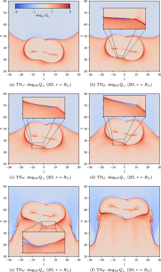
Figure 9. Maps of slog10 Q⊥ in blue–white–red color scale against the unrolled polar (ζ–η) coordinates on the photosphere depicting the topological evolution of the TN configuration in six sequential snapshots, TN1–TN6, in panels (a)–(f). Cutouts in panels (b)–(e) indicate the accumulation of reconnected open (blue) flux on the trailing edge of the separatrix dome. In panel (b), the flux is isolated to a small patch near the footprint of the trailing spine of NC . In panels (c) and (d), the extent of the reconnected open flux has increased, forming a narrow corridor that extends around the left side of the dome only. In panel (e), the reconnected open flux has been extended to the right as well, forming a narrow corridor that now surrounds the entire dome.
Download figure:
Standard image High-resolution imageIt is interesting to compare the amounts of open flux reconnected into the satellite coronal hole in the two cases. We do this by comparing the areas of the blue flux domains on the trailing edges of the dome footprints in states SN3 (panel (f) of Figure 7) and TN5 (panel (e) of Figure 9). Here TN5 corresponds to an earlier simulation time than SN3, so the fact that the coronal hole appears larger in the TN case suggests that more flux has reconnected in a shorter period of time. We have confirmed this by examining the S-Web maps of the outer boundary in the two cases and comparing the area bounded by the closed curves of the HCS and the high-Q arcs that form. In the SN configuration, this arc is composed of the flux from the narrow corridors along the boundary of the dome footprint, whereas in the TN case, it involves those corridors and also the separatrix curtain of NC . In both cases, the enclosed flux emanates from the satellite coronal hole, but the amount is significantly greater for TN5 than for SN3. This confirms that more flux has reconnected in a shorter period of time in the TN case.
5. Implications for Observations and the S-Web
The results presented here have important implications for both remote-sensing and in situ observations of the corona and wind. Three types of observations are most relevant to our simulations and are commonly used to reveal the dynamics of the large-scale corona and SSW: disk images of evolving coronal-hole structures (Harvey & Recely 2002), coronagraph observations at the limb of the outer corona and inner heliosphere (Wang 2014), and in situ measurements of the SSW (Zurbuchen 2006). Coronal-hole evolution is generally measured by either direct detection of the holes via X-ray imaging or inference of the holes by combining photospheric magnetograms with steady-state source-surface or MHD models (Wallace et al. 2020). The latter method is necessarily model-dependent, but detailed comparisons between the PFSS and MHD models and observed X-ray coronal holes appear to show good agreement, at least for coronal holes that are clearly resolved in images (Riley et al. 2006).
From Figure 9 and, to some extent, Figure 7, we observe that the disk signature of a newly forming pseudostreamer is the spontaneous appearance of a satellite coronal hole deep in the closed-field region, apparently well detached from the main polar hole. For the system that we simulated, the satellite hole initially forms with vanishing area, so its early growth would be difficult to observe directly in X-ray images. Given the resolution of present instruments and the obscuration of coronal holes by neighboring closed flux, a coronal hole generally must be of order 10'' or larger in size to be clearly visible. The satellite hole in Figure 9 is long and narrow, but it should be detectable in X-ray images by the third panel or so (Figure 9(d)). Although the satellite hole would appear disconnected from the main polar hole, in fact, there is a narrow corridor of open flux that connects them by the time of Figure 9(d). Even before this time, the holes are connected, on the photosphere by the separatrix curve of the parasitic polarity and in the corona through the various nulls and fan surfaces. Again, however, these structures would be difficult to observe in coronal images. These arguments imply that the earliest and most effectively observed disk signature of pseudostreamer formation is likely to be the presence of a large parasitic polarity near a coronal-hole boundary. Hence, it may not be possible to observe the satellite hole when it first forms, but as soon as a parasitic region that was originally deep within the HS moves near the coronal-hole boundary, as in Figure 9(a), the formation of a pseudostreamer inevitably follows. Furthermore, a change in the solar-wind plasma composition in the heliosphere will inevitably follow, as discussed below.
In principle, high-resolution magnetograms combined with source-surface maps provide a more sensitive detection of coronal-hole formation. There is no obscuration by overlying coronal structures because the maps rely only on photospheric magnetograms; however, the maps are model-dependent. Since the source-surface model assumes that the corona has no electric currents, the closed flux cannot have any stress, ruling out the evolution shown in Figures 7–9. In Figure 9, for example, some of the closed flux under the HS has clearly moved poleward and, consequently, developed magnetic stress in the form of volumetric electric currents. The source-surface model would remove this stress by simply opening the flux, so the narrow coronal-hole corridor that forms between the parasitic polarity and the closed HS flux would be much broader. Photospheric vector magnetograms, however, show that the coronal magnetic field is nonpotential, certainly in the vicinity of filament channels, but also more generally within the volume of active regions (Schrijver et al. 2005). Although the qualitative features of the evolution may be similar for the source surface and our model, the quantitative results are certain to be very different; a series of potential-field states (e.g., Titov et al. 2011) will not conserve key topological constraints such as magnetic helicity, nor will it capture the development of magnetic stress that plays an important role in determining open versus closed flux. For detailed comparison with data, therefore, a fully dynamic model such as ours, which includes the history of the evolution, is essential.
A key feature of the dynamic evolution is that it is primarily due to interchange reconnection between the closed field of the parasitic polarity and the open flux in front of it. The result that interchange reconnection plays a dominant role in the open/closed flux evolution agrees well with the findings of many previous observational and theoretical studies (e.g., Wang et al. 1998; Crooker et al. 2002; Higginson et al. 2017a). It is due to interchange reconnection that the satellite hole appears deep in the closed-field region and grows from zero size. Furthermore, the reconnection limits the possible size of the satellite hole, as is evident by inspecting panels (a) and (b) of Figure 5. The relevant interchange reconnection is between the blue open flux north of the parasitic polarity and the red closed flux overlying the southern part of the PIL of the parasitic region. The interchange reconnection converts this red flux into the open flux of the satellite hole, but because there is a finite amount of this flux, in the absence of coincidental flux emergence in this region, the size of the satellite hole is limited. In our simulation, we remain very far from reaching this limit, but the conclusion is clear: the type of evolution calculated in this paper will tend to produce small satellite coronal holes and, therefore, pseudostreamers that lie near the main HS.
It is possible to produce larger satellite holes through the type of evolution described by Antiochos et al. (2011) and Titov et al. (2011), where one starts with an "elephant trunk" coronal hole. When a parasitic-polarity region moves across the trunk, the bottom section of the trunk is converted into a satellite hole. We did not simulate this case, because the elephant-trunk configuration already resembles a pseudostreamer depending on the width of the trunk. As the trunk narrows, it is not possible to determine uniquely when the structure converts from a single highly convoluted streamer to a streamer plus a pseudostreamer. In this case, even the ideal "squeezing" of the corridor can result in the appearance of a pseudostreamer. Our simulation, however, starts with an isolated streamer, and the pseudostreamer forms when the separatrix flux (spines or fan, as the case may be) of the parasitic region first breaks through into the open field. In this case, the pseudostreamer appearance and formation require reconnection and are clearly defined.
To be sure, our pseudostreamer first appears with vanishingly small size, but Figure 9 demonstrates that the timescales for its growth allow the process to be readily observed by combining disk and coronagraph images. Figure 10 shows the expected appearance of the pseudostreamer evolution in coronagraph images (panels (c), (f), and (i)) and the S-Web arc structure in the heliosphere (panels (a), (d), and (g)). Both depend explicitly on the structure of the S-Web, which is shown in the 3D rendering of slog10 Q⊥ in panels (b), (e), and (h). We note from Figures 9 and 10 that the parasitic polarity needs to migrate a distance of order its width, ∼105 km, to produce an observable satellite coronal hole on the disk and a pseudostreamer that is well separated from the streamer on the limb. Assuming a typical "drift" velocity for the parasitic polarity of ∼0.5 km s−1, we estimate that the pseudostreamer growth time is of order a day or two. Consequently, it should be possible to test our findings by looking for cases where no pseudostreamer is visible on the east limb, but a large parasitic region is observed to drift toward a coronal-hole boundary during the 10 days or so of disk passage, resulting in a pseudostreamer appearing on the west limb. Observations by a combination of Earth-based telescopes and Solar Orbiter (Müller et al. 2013), which contains both magnetographs and coronagraphs and can achieve near corotation for several days, would be ideally suited for this observational test of our model. Such observations would be able to determine quantitatively whether the interchange reconnection that we calculate is too efficient or inefficient compared to that occurring on the Sun. We discuss this point in more detail below.

Figure 10. Maps of slog10 Q⊥ against unrolled polar (ζ, η) coordinates on the source surface (left column) depict the evolution of an S-Web arc through three representative snapshots (TN1, TN3, and TN5) in the top, middle, and bottom rows, respectively. The underlying 3D structure, with representative field lines, is shown by the translucent volume rendering in the middle column, where the HCS is clearly visible as the bold red curve at the apex of the HS, while the arc from the left column is actually the imprint of a ribbon-like surface that extends down into the volume. In the right column, the same structure has been rotated onto the limb and rendered as a line-of-sight integrated quantity, weighted by a Gaussian emissivity with a half-width of 10° from the plane of the sky.
Download figure:
Standard image High-resolution image
In situ measurements from Solar Orbiter and, even more so, Parker Solar Probe, which samples the solar-wind plasma very near the Sun before propagation effects obscure its origins, will also be highly revealing when compared with our model. As discussed in the Introduction, the slow wind originates near the open/closed boundary and is widely believed to be due to the release of closed-field plasma onto open field lines, most likely by interchange reconnection (Higginson et al. 2017a, 2017b). At the open/closed boundary of an isolated streamer, the interchange reconnection will involve the large, outermost closed loops of the HS; at the boundary of an isolated pseudostreamer, on the other hand, the interchange reconnection will involve the shorter, active-region-like loops of the parasitic polarity. The properties of the plasma in these two types of closed loops will almost certainly be different—the parasitic-polarity loops will have higher temperatures and densities and, most likely, the corresponding FIP properties as well. For example, it has been reported that streamer plasma shows evidence of gravitational settling (Raymond et al. 1998), which is definitely not the case for active regions. This is where our configuration, in which we start with a pure streamer (no coronal-hole corridor), is particularly important. Our model predicts that as the parasitic polarity approaches the streamer boundary (e.g., the situation in Figure 10(c)), the solar-wind plasma composition will clearly transition from typical quiet-Sun plasma to the higher freeze-in temperatures and changes in the FIP bias indicative of active regions. There will be a period of time, roughly the timescale in going from panels (c) to (f) in Figure 10, during which the plasma will have characteristics of both the streamer and pseudostreamer slow wind. As the parasitic region moves further into the open flux (e.g., from panels (f) to (i) in Figure 10) and the S-Web arc becomes well separated from the HCS (as in Figure 10(g)), so the plasma properties near the HCS should revert back to those extant before the appearance of the pseudostreamer.
In principle, it should be possible to perform even more stringent tests of pseudostreamer formation by using spectroscopic instruments, such as SPICE on Solar Orbiter (Spice Consortium et al. 2020), to determine the composition of sources in the corona in combination with in situ composition measurements in the wind. This will require a somewhat fortuitous positioning of the spacecraft, but given that parasitic-polarity regions are commonly observed to migrate toward the polar coronal holes, it may well be possible to capture some events similar to the evolution calculated here. Note that such tests of the S-Web are not limited to only pseudostreamer appearance; the whole growth phase can be effective. Consider, for example, a spacecraft that is near corotation and positioned somewhat north of the HCS in Figure 10(a). As the S-Web arc grows from panel (a) to (g) and sweeps across the spacecraft, the plasma would first exhibit fast-wind composition, then slow as the S-Web arc intersects the spacecraft, then go back to fast. Even if the spacecraft is not corotating, as long as its trajectory is known and the dynamics of the S-Web are well constrained, the solar-wind properties can be predicted. In combination with numerical simulations such as the ones presented here, observations from Solar Orbiter and Parker Solar Probe could provide definitive tests not only of pseudostreamer formation but of the full S-Web model for slow-wind formation.
6. Discussion and Conclusions
In this paper, we have simulated the simplest and most generic mechanism for forming large solar pseudostreamers: the migration of a large parasitic-polarity region from fully inside the closed field of an HS into the open field of a neighboring coronal hole. Emergence of bipolar flux from below the photosphere is a mechanism for the ubiquitous formation of pseudostreamers within coronal holes, but such structures typically are much smaller in scale than those considered here. For simplicity, we investigated the magnetohydrodynamic evolution of the inner corona in the context of a source-surface model for the magnetic field, r ≤ RSS = 3 R⊙, as our focus is on the magnetic structure and reconnection dynamics. In this model, the effect of the solar wind is imposed through boundary conditions on the magnetic field, rather than directly through a radial outflow. Detailed calculations of the outflowing solar wind would require nonreflecting radial boundary conditions and a much larger spatial domain, but this wind would have no significant impact on the pseudostreamer formation process in the inner corona. Higher in the corona, we expect the curvature of the magnetic field to differ somewhat between the model presented here and a self-consistent wind solution; the inertial force of the wind will tend to straighten field lines within the coronal volume, where our model imposes this condition only at the source surface. However, this should have no effect on the topology of the magnetic field and minimal impact on its morphology. Despite these simplifications, the simulation results presented here have several important consequences for understanding the corona and heliosphere, revealing as they do the characteristic dynamics of pseudostreamer formation and the expected observational signatures of this evolution.
We considered two relevant topologies for the parasitic polarity: an embedded bipole with a fan surface and spine lines emanating from a single null point (e.g., Antiochos 1990; Lau & Finn 1990; Priest & Titov 1996) and a more extended region with three null points connected by separator lines (e.g., Titov et al. 2011). From a topological perspective, the key difference between the two cases is that the SN configuration has only a 1D outer spine line extending to a very distant closed region or out into the heliosphere; the TN configuration, on the other hand, has a 2D fan curtain bounded by spine lines on either side. Although we anticipated that the two cases might exhibit very different rates of reconnection and magnetic restructuring, notice that the geometrical difference between the two cases is not dramatic, as can be seen from Figure 2. For the triple-null case in the right panels, the outer distant connection clearly appears to be via a 2D ribbon (white field lines); even for the SN case in the left panels, however, the connection appears to have some linear extent, albeit definitely smaller. As can be seen in Figures 2(c) and (e), the high-Q region inside the parasitic-polarity region resembles a line segment, just as in the TN case, rather than a single point. The single-null point has highly asymmetric eigenvalues (Fukao et al. 1975), leading to spine lines with a "preferred" direction along the long axis of the elliptical parasitic-polarity region (Pontin et al. 2016).
Although the qualitative dynamics of the two cases are fairly similar, in that they are dominated by interchange reconnection through the deformed nulls and separators, the quantitative differences are important. As can be seen from a comparison of Figures 6 and 8, the amount of interchange reconnection is measurably greater for the TN case. Current sheets form all along the separator lines, thereby enlarging the region over which reconnection occurs. We conclude, therefore, that the shape of the parasitic-polarity region and the distribution of flux within its PIL will play a major role in pseudostreamer formation. A highly elliptical parasitic-polarity region with multiple nulls will form a satellite coronal hole and pseudostreamer more rapidly than a circular polarity region, even if the latter has more flux. This effect should provide a distinctive observational test of our model, especially in comparison to the source-surface or other equilibrium models. Furthermore, it implies that accurate models for the large-scale corona and inner heliosphere need to be able to resolve the photospheric flux distribution fairly accurately. For example, if the flux distribution of the TN case in Figure 2 is not resolved into its two maxima, then even if the total flux is conserved, the resulting coronal topology would incorrectly exhibit only a single null.
For both the TN and SN cases, we find that the reconnection dynamics are smooth, with little evidence of burstiness or 3D island formation. This is mainly due to the slow driving of the system, v ≪ vA , so that the current sheet buildup is slow. In this case, the system can achieve a quasi-steady state where the interchange reconnection balances the driving until the reconnected flux starts to run out, as discussed above. This condition is obeyed even more stringently on the Sun, where the driving velocities are only ∼1 km s−1, some three orders of magnitude smaller than the typical coronal Alfvén speed, vA ∼ 1000 km s−1. In other investigations of reconnection in null-point topologies, we have noted copious magnetic island formation in both numerical simulations (Wyper et al. 2016) and observations (Kumar et al. 2019). In those investigations, however, the reconnection was driven by a fast Alfvénic eruption, either a jet or a coronal mass ejection. The free energy was associated with the large volumetric currents of a filament channel inside the polarity region. The large-scale driving of Figure 3, in contrast, tends to induce currents only at the boundary between the parasitic-polarity region and the surrounding flux and does not build up a filament channel.
The result that our reconnection is laminar has potentially critical implications for understanding the recent discovery by Parker Solar Probe of so-called switchbacks in the solar wind (Bale et al. 2019; Kasper et al. 2019; Mozer et al. 2020). Some authors have argued that the switchbacks are due to interchange reconnection that produces either magnetic islands (Drake et al. 2020) or highly kinked field lines (Zank et al. 2020). We would argue that, outside of streamers, our model calculates the most common and largest-scale interchange reconnection in the corona and, therefore, the most likely to lead to switchbacks. Our simulations show copious interchange reconnection but no evidence for plasmoids or switchback structures. Very close to the current sheet, the just-reconnected field lines have large kinks—this is the defining characteristic outcome of reconnection—but the kinks do not survive propagation to significant heights and do not grow into actual switchbacks. On the basis of these calculations, at least, it appears unlikely that quasi-steady interchange reconnection in pseudostreamers, of the laminar type, shown here is the mechanism for switchback formation.
A caveat to this conclusion is that the Lundquist number of our simulations is in the range 102–103, many orders of magnitude less than that of the corona. As a result, the current sheets at the nulls and separators never develop a large aspect ratio before reconnection sets in. For example, the current sheet in Figure 5 has an aspect ratio a ≈ 10; for either the tearing (Furth et al. 1963) or plasmoid (Loureiro et al. 2007) instability, in contrast, aspect ratios a > 100 are required. It is highly likely that if we were to perform this simulation with progressively higher numerical refinement, we eventually would find that magnetic islands form and are ejected outward along the open flux. On the other hand, for increasing numerical refinement, the current sheet width at reconnection onset decreases, and the magnetic islands would tend to be small and less likely to survive propagation to significant heights. Further grid-refinement studies are needed in order to determine definitively whether the small-scale magnetic islands formed in this way contribute significantly to the formation of switchbacks.
Another important conclusion from our results is that the formation process of pseudostreamers cannot be represented accurately as a series of equilibrium states from either the source-surface or steady-state MHD models. The reason is straightforward and inescapable: the large-scale photospheric motions that drive a parasitic polarity into a coronal hole also introduce stress into the closed field. We expect that the evolution predicted in Figure 10, for example, will be qualitatively the same for all models. On the limb, the pseudostreamer will first be noticeable as a slight bulge on one side of the streamer, Figure 10(f), which slowly splits into a distinct pseudostreamer stalk well separated from the streamer itself, Figure 10(i). This evolution is reflected in the heliosphere, where a very small S-Web arc first appears somewhere on the HCS (Figure 10(d)). This is so near to the HCS that we would not expect to see any fast wind separating this arc and the HCS. However, the arc continues to grow, so that by the time of Figure 10(g), a fast-wind region should be enclosed between the arc and the HCS. This developing 3D structure of the S-Web arc is shown in Figures 10(e) and (h).
Although the qualitative evolution of Figure 10 is generic to all models, the quantitative details are likely to be very different between the equilibrium and our fully dynamic model. Consequently, for comparing with in situ measurements, the equilibrium models will have inherent errors. This may be one of the main reasons that the mapping of heliospheric plasma back down to its coronal origin has long proved to be a challenge, even for Parker Solar Probe when it is only tens of solar radii from the Sun (Badman et al. 2020). We conclude, therefore, that highly accurate forecasting/nowcasting of the heliosphere, such as predicting particle radiation for interplanetary spacecraft and astronauts, will require a fully dynamic model that includes the time-dependent photospheric magnetic and velocity fields. This conclusion is also subject to the caveat stated earlier on the effect of numerical resolution, but, if anything, a higher Lundquist number would only increase the discrepancies between the equilibrium and fully dynamic models.
A key issue that remains to be addressed is the effect on our model of small-scale photospheric motions, in particular, the supergranules. They have flow speeds similar to that of the large-scale flows driving the "rush to the poles," but they are incoherent at scales larger than 30,000 km, smaller than the parasitic region in Figure 2. These motions are believed to be critical for the slow-wind origin because they drive the constant interchange reconnection that releases closed-field plasma along all parts of an open/closed boundary (Higginson et al. 2017a, 2017b). Because resolving the convective motions numerically along with the large-scale evolution would be prohibitive computationally, we did not include them in our model. However, there is no doubt as to their importance. The impact of the small-scale motions on our conclusions is far from clear. On the one hand, we expect they would break up any large-scale current sheets, such as those in Figure 5, and enhance the effective reconnection rate. This suggests that the dynamic pseudostreamer formation process would be closer to the equilibrium model than implied by our results presented here. Also, it seems even less likely that the interchange reconnection would give rise to coherent structures that can explain the switchbacks. On the other hand, the small-scale motions are likely to inject more stress into the closed field, so the system is farther from the potential-field state of the equilibrium models. If the motions also inject net helicity, this would lead to filament-channel formation and eruptive events (Dahlin et al. 2019). We conclude, therefore, that an important next step in understanding the corona and slow wind is to add the small-scale convective motions, perhaps only with a statistical approach, to the large-scale flows of our model for the dynamic formation of pseudostreamers.
The bulk of the work for this study was performed while R.B.S. and D.I.P. held positions at the University of Dundee and were supported by the UK's STFC under grant ST/N000714/1. R.B.S. is currently supported by the Office of Naval Research 6.1 program and the Theory and Modeling task under NRL's WISPR grant (NNH11EK11I) from NASA. S.K.A. and C.R.D. were supported in part by NASA H-LWS and H-SR grants. The authors would like to thank the anonymous referee for the careful reading of the manuscript and valuable insights.
Appendix
The analytical surface flow used to advect the photospheric flux is described here in detail. The components of the velocity have a functional form given by
and
where
is a Gaussian distribution function and

is its derivative with respect to the independent variable (ζ or η, depending on the case). This analytical flow field is guaranteed to be divergence-free, provided that Aζ = −Aη , irrespective of the other arguments, and it becomes asymptotically small at large distances from the reference positions (ζc and ηc ).
Due to the separability of the flow, the peak poleward speed set by each circulation region is given as
The combined flow pattern is a superposition of four overlapping flow fields, two in each hemisphere, with the specific parameters given in Table 3, which gives a peak driving speed of  in the overlapping regions.
Table 3. Parameters of Imposed Surface Flows
| ζ− | ζ+ | ζc | kζ | Aζ | η− | η+ | ηc | kη | Aη | |
|---|---|---|---|---|---|---|---|---|---|---|
| 1 | −81.0° | +36.0° | −22.5° | 49. | +10. | −108.0° | +108.0° | +45.0° | 40. | −10. |
| 2 | −36.0° | +81.0° | +22.5° | 49. | −10. | −108.0° | +108.0° | +45.0° | 40. | +10. |
| 3 | −81.0° | +36.0° | −22.5° | 49. | −10. | −108.0° | +108.0° | −45.0° | 40. | +10. |
| 4 | −36.0° | +81.0° | +22.5° | 49. | +10. | −108.0° | +108.0° | −45.0° | 40. | −10. |
Note. Flow position parameters are given in degrees of simulation latitude (ζ) and longitude (η); velocity amplitudes are given in rad km s−1.
Download table as: ASCIITypeset image
Footnotes
- 6
Note that all topological descriptions are model-dependent, as they require instantaneous knowledge of the entire magnetic field.