


Abstract
Yellowballs (YBs) were first discovered during the Milky Way Project (MWP) citizen science initiative. The MWP users noticed compact, yellow regions in Spitzer Space Telescope mid-infrared (MIR) images of the Milky Way plane and asked professional astronomers to explain these "yellow balls." Follow-up work by Kerton et al. determined that YBs likely trace compact photodissociation regions associated with massive and intermediate-mass star formation. The YBs were included as target objects in a version of the MWP launched in 2016, which produced a listing of over 6000 YB locations. We have measured distances, cross-match associations, physical properties, and MIR colors of ∼500 YBs within a pilot region covering the l = 30°–40°, b = ±1° region of the Galactic plane. We find that ∼20%–30% of YBs in our pilot region contain high-mass star formation capable of becoming expanding H ii regions that produce MIR bubbles. A majority of YBs represent intermediate-mass star-forming regions whose placement in evolutionary diagrams suggest they are still actively accreting and may be precursors to optically revealed Herbig Ae/Be nebulae. Many of these intermediate-mass YBs were missed by surveys of massive star formation tracers; thus, this catalog provides information for many new sites of star formation. Future work will expand this pilot region analysis to the entire YB catalog.
Export citation and abstract BibTeX RIS
1. Introduction
Yellowballs (YBs), named for their appearance in Spitzer Space Telescope 4.5–8.0–24 μm mid-infrared (MIR) images, were originally discovered by citizen scientists working on the Milky Way Project (MWP; Simpson et al. 2012). The only study of YBs to date, Kerton et al. (2015, hereafter KWA15), attempted to answer the citizen scientists' question, "What are these yellow balls?" by showing that YBs likely represent young photodissociation regions (PDRs) associated with intermediate and massive star-forming regions. They proposed a sequence in which some fraction of YBs will later expand their PDRs and become MIR bubbles.
KWA15 cataloged 928 YBs identified by MWP participants and used infrared photometry, together with cross-matching YBs with various catalogs, to explore YB properties. Since YBs were a serendipitous discovery, the original MWP tools were not designed with them in mind, and the MWP tutorial materials did not instruct users to identify YBs or provide them with interactive tools to accurately measure YB angular sizes.
Although sizes were included in the KWA15 study, at best these were rough upper limits to the actual angular sizes of the YBs. Also, since users identified these objects on an ad hoc basis, there was no expectation that the resulting catalog was complete. Cross-matches of YBs with catalogs produced by the Bolocam Galactic Plane Survey (BGPS; Aguirre et al. 2011) and the APEX Telescope Large Area Survey of the Galaxy (ATLASGAL; Csengeri et al. 2014) indicated that nearly all of the KWA15 YBs are associated with dense gas. Additionally, ∼65% of the KWA15 YBs have counterparts in the Wide-field Infrared Survey Explorer (WISE) catalog of Galactic H ii regions (Anderson et al. 2014) and ∼34% in the Red MSX Source (RMS) catalog (Lumsden et al. 2013) to within a 24'' cross-match distance. Most of the YBs reported in KWA15 appear in environments associated with star formation, such as infrared dark clouds (IRDCs), and/or in close proximity to the bubbles representing expanding H ii regions (Simpson et al. 2012).
The IR photometry of KWA15 indicated that many YBs have higher flux densities at 8 μm than 12 μm, with flux densities rising again toward longer IR wavelengths. The brightness of these objects at 8 μm could be explained if YBs are dense, young PDRs containing a high fraction of ionized polycyclic aromatic hydrocarbon (PAH) emission (e.g., Roelfsema et al. 1996). This could also explain why many YBs do not have counterparts in the RMS catalog (Lumsden et al. 2013), since having rising spectral energy distributions (SEDs) across MIR MSX wavelengths was employed as one criterion for inclusion in the RMS catalog. For a sample of 138 YBs that had counterparts in the RMS catalog and good distance estimates, KWA15 found that these YBs had typical diameters of 0.1–1 pc and luminosities of 103–106 L⊙. However, this sample was likely biased to luminous objects, since the RMS survey targeted the identification of massive young stellar objects (MYSOs), complete to typical B0 stars at the distance of the Galactic center (Lumsden et al. 2013).
Based on their findings, KWA15 argued that YBs represent young PDRs associated with intermediate and massive star-forming regions. However, KWA15's results raised new important questions about the nature of YBs. Does the RMS-selected sample from KWA15 accurately represent the YB luminosity and mass distribution? What are the properties of the protostellar clumps associated with YBs? What fraction of the YBs contain the massive stars that will eventually form mature H ii regions and large MIR bubbles?
To address these questions, a more intentional MWP study was developed to focus on YBs. The user interface was redesigned to include a tool that both identified YBs and measured their sizes. The second data release (MWP DR2) also includes a new catalog of bubbles and bow shocks driven by OB stars (Jayasinghe et al. 2019). This paper focuses on a pilot study utilizing a 20 deg2 subset of the DR2 YBs. Analysis of the complete DR2 YB catalog will be addressed in a subsequent paper. In addition to resolving questions about the nature of YBs, the YB catalog will provide a new, extensive catalog containing the properties of thousands of star-forming regions. Many of these regions, particularly in the intermediate-mass range, have not been studied or cataloged before.
The current list of DR2 YBs and our motivation for analyzing a subset of these objects prior to addressing the entire survey are discussed in Section 2. A comparison of DR2 YBs with existing catalogs tracing star-forming regions and dense gas structures is described in Section 3.1. Our derivation of YB distances is presented in Section 3.2, and the physical properties of interstellar medium clumps associated with YBs are summarized in Section 3.3. Our photometry procedure is described in Section 3.4, and the results of a 2D Gaussian fitting routine we employed to assess the accuracy of user-measured sizes and quantify the deviation of features from those expected for young PDRs are presented in Section 3.5. Our analysis and discussion of YB properties are presented in Section 4.
Our conclusions are presented in Section 5.
2. A First Look at YBs in MWP DR2
The original MWP launched in 2010 as the ninth online research program hosted through the Zooniverse suite of citizen science programs (Simpson et al. 2014). The MWP was created to enable large statistical studies of Galactic star formation using MIR data from the Spitzer GLIMPSE (Benjamin et al. 2003) and MIPSGAL (Carey et al. 2009) surveys. The original release of the MWP focused on identifying and measuring MIR bubbles (Simpson et al. 2012). In this original data analysis, YBs were identified by users as interesting but unexplained objects. Users flagged these objects for examination by astronomers. Follow-up investigation resulted in the work presented in KWA15.
In 2016 September, an implementation of the MWP was released to citizen scientists that included the identification and measurement of YBs and bow shocks produced by winds from OB stars as two additional key science objectives. Citizen scientists were trained to mark the center location and angular size of YBs in Spitzer 4.5–8.0–24 μm images.
Employing this new tool, users searched for YBs in images from the Spitzer GLIMPSE and MIPSGAL legacy surveys of the inner Galactic plane (∣l∣ < 65°); the Cygnus-X legacy survey, an approximately 24 deg2 region (centered on l ∼ 79 3, b ∼ 1°) of one of the richest known star-forming regions in our Galaxy (Hora et al. 2007; Beerer et al. 2010); and the SMOG legacy survey (Carey et al. 2008), which covers a 21 deg2 (l = 102°–109°, b = 0°–3°) area of a representative region of the outer Galaxy.
The MWP history, interface, images, workflow, and identification tools, as well as the construction of the MWP DR2 bubble and bow shock catalogs, are presented in detail in Jayasinghe et al. (2019). Here we summarize specifics for producing the current list of YBs. Citizen-scientist classifications were aggregated to produce individual catalog entries for any given object. The MWP data reduction pipeline used the density-based clustering algorithm DBSCAN (Ester et al. 1996) with a 0002 clustering radius to identify YBs, identical to the process used to produce the DR1 small bubble catalog (Simpson et al. 2012). In this pipeline, a minimum of five classifications were needed to identify a YB cluster. For each cluster, the Galactic longitude (l), Galactic latitude (b), and YB radius (r) were averaged. The uncertainties in these parameters were calculated based on their standard deviations among the classifications in each cluster. The hit rate for a given cluster is the ratio of the total number of classifications in the cluster to the total number of times images containing the classified object were viewed by MWP users. The DR2 YBs were identified from images at the highest zoom level only (015 × 0075).
The complete list of DR2 YBs is presented in Table 1. It contains 6176 YBs, more than six times the number of YBs investigated by KWA15 and more than twice the number of bubbles in the DR2 catalog. It includes the YB position in Galactic coordinates, user-measured YB radius in degrees, dispersion in YB position in degrees, dispersion in YB radius in degrees, and hit rate. This list includes all identified YBs. The lowest reported hit rate is 0.05; however, 6050 YBs have hit rates >0.125, the cutoff employed for DR2 bubbles. We discuss the relationship between different measurements used to estimate YB sizes in Section 4.3. We will refer to the user-defined radius as the MWP radius hereafter. No filtering has yet been applied to remove spurious objects and produce a final version of the YB catalog. Instead, in this paper, we present a pilot study that uses all YBs identified by citizen scientists in the l = 30°–40°, b = ±1° region to develop methods for assessing the reliability of citizen-scientist identifications and automating procedures to analyze the entire YB catalog.
Table 1. DR2 YBs
| YB | Gal. Longitude | Gal. Latitude | MWP Radius | σl | σb | σr | Hit |
|---|---|---|---|---|---|---|---|
| Number | (deg) | (deg) | (deg) | (deg) | (deg) | (deg) | Rate |
| 1 | −0.04143 | 0.16705 | 0.00366 | 0.00077 | 0.00073 | 0.0020 | 0.65 |
| 2 | −0.02311 | 0.16916 | 0.00391 | 0.00056 | 0.00053 | 0.0014 | 0.48 |
| 3 | 0.04088 | 0.02020 | 0.00314 | 0.00019 | 0.00037 | 0.00094 | 0.23 |
| 4 | 0.18604 | −0.61181 | 0.00304 | 0.00071 | 0.00036 | 0.0025 | 0.19 |
| 5 | 0.20075 | −0.51336 | 0.00222 | 0.00050 | 0.00045 | 0.00090 | 0.29 |
| 6 | 0.20950 | −0.00195 | 0.00334 | 0.00039 | 0.0010 | 0.00079 | 0.17 |
| 7 | 0.27904 | −0.48463 | 0.00659 | 0.00055 | 0.0010 | 0.0019 | 0.63 |
| 8 | 0.31351 | −0.20354 | 0.00456 | 0.00078 | 0.00078 | 0.0016 | 0.53 |
| 9 | 0.31413 | −0.19272 | 0.00459 | 0.00079 | 0.0010 | 0.0021 | 0.50 |
| 10 | 0.33171 | −0.06248 | 0.00442 | 0.00084 | 0.00033 | 0.0020 | 0.29 |
Only a portion of this table is shown here to demonstrate its form and content. A machine-readable version of the full table is available.
Download table as: DataTypeset image
Jayasinghe et al. (2019) employed criteria to determine whether bubbles and bow shocks identified by citizen scientists would be included in the DR2 catalogs and set reliability flags for objects that were included. These criteria were developed based on prior identifications or knowledge of these objects. In the case of YBs, it is not possible to use the DR1 YB catalog to help assess the reliability of DR2 identifications for two reasons. First, identifications of DR2 YBs were made at four times the resolution of DR1 YBs, which greatly affects the types of objects that might be identified as round and compact in the images. Second, citizen scientists were never specifically asked to search for YBs in DR1, so comparing hit rates between DR1 and DR2 lacks meaning.
Thus, we have opted to perform an initial analysis of all of the YBs that were included in the l = 30°–40°, b = ±1° region after clustering and averaging was performed. This region contains 516 YBs, with a negligible 10 YBs that achieved hit rates less than the 0.125 cutoff employed for DR2 bubbles. The region was chosen because it is covered in numerous other Galactic plane surveys and overlaps with multiple catalogs, which are discussed further in Section 3.1.
3. Results
3.1. Catalog Cross-matches
To help identify those YBs that are most likely associated with regions of star formation, we cross-matched the 516 YBs in our pilot region with catalogs of star-forming regions and interstellar medium structures produced from surveys covering this region. We used the Hi-GAL compact source catalog of Elia et al. (2017, hereafter EMS17) containing 4764 sources within the pilot region, the GaussClump Source Catalogue from ATLASGAL (624 sources; Csengeri et al. 2014), the Co-Ordinated Radio "N" Infrared Survey for High-mass star formation catalog (CORNISH, 494 sources; Purcell et al. 2013), the RMS catalog (210 sources; Lumsden et al. 2013), and the WISE Catalog of Galactic H ii Regions (672 sources; Anderson et al. 2014).
The Hi-GAL and ATLASGAL catalogs both identify compact core and clump structures in the interstellar medium using infrared and submillimeter images, respectively. Not surprisingly, 93% of the ATLASGAL associations are also Hi-GAL associations. The CORNISH, RMS, and WISE catalogs were all primarily focused on the discovery of regions of higher-mass star formation using radio and infrared emission. CORNISH detected 5 GHz radio emission from H ii regions and is complete to emission from Galactic sources for B2 and earlier stars. The RMS used infrared colors and fluxes to identify potential high-mass star-forming regions and is complete to Galactic sources with luminosities corresponding to embedded B0 stars. The WISE catalog was constructed by identifying H ii region candidates via searching for their characteristic MIR morphology. Exact completeness limits are hard to define for the WISE catalog, but we expect it to include lower-luminosity sources that did not meet the detection limits of the CORNISH and RMS catalogs.
The catalogs were obtained from project-specific websites or the VizieR catalog access tool, and the cross-matching was done with TOPCAT (Taylor 2005). A best-match symmetric option was chosen to allow for only one-to-one matches, and a match radius of 24'' (the average angular diameter of the YBs as defined by the citizen scientists) was used. We found 385 Hi-GAL matches, 162 ATLASGAL matches, 59 CORNISH matches, 88 RMS matches, 263 WISE matches, and 74 objects lacking matches in any of these catalogs. The resulting cross-matches are listed in Table 2.
Table 2. YB DR2 Pilot Region Cross-matches
| YB | Gal. Longitude | Gal. Latitude | Hi-GAL ID | AGAL ID | CORNISH ID |
|---|---|---|---|---|---|
| Number | (deg) | (deg) | |||
| 1153 | 30.0033 | −0.2658 | HIGALBM30.0033–0.2654 | G030.0027–0.2643 | ⋯ |
| 1154 | 30.0233 | −0.0428 | HIGALBM30.0254–0.0389 | ⋯ | ⋯ |
| 1155 | 30.0242 | 0.1085 | HIGALBM30.0230+0.1088 | G030.0209+0.1048 | ⋯ |
| 1156 | 30.0325 | 0.1079 | HIGALBM30.0323+0.1082 | ⋯ | ⋯ |
| 1157 | 30.0558 | −0.3390 | ⋯ | ⋯ | ⋯ |
| 1158 | 30.0670 | 0.0976 | HIGALBM30.0650+0.0991 | ⋯ | ⋯ |
| 1159 | 30.0954 | 0.0440 | HIGALBM30.0958+0.0440 | ⋯ | ⋯ |
| 1160 | 30.1139 | −0.5646 | ⋯ | ⋯ | ⋯ |
| 1161 | 30.1319 | −0.6586 | HIGALBM30.1324–0.6578 | ⋯ | ⋯ |
| 1162 | 30.1971 | 0.3085 | HIGALBM30.1971+0.3101 | G030.1963+0.3107 | ⋯ |
| CORNISH Type | RMS ID | RMS Type | WISE ID | WISE Type |
|---|---|---|---|---|
| ⋯ | ⋯ | ⋯ | G030.003–00.267 | C |
| ⋯ | 3110 | Diffuse H ii region | G030.022–00.042 | K |
| ⋯ | 3092 | Diffuse H ii region | G030.026+00.109 | K |
| ⋯ | ⋯ | ⋯ | ⋯ | ⋯ |
| ⋯ | ⋯ | ⋯ | G030.055–00.339 | C |
| ⋯ | ⋯ | ⋯ | G030.067+00.097 | Q |
| ⋯ | ⋯ | ⋯ | G030.090+00.044 | Q |
| ⋯ | ⋯ | ⋯ | ⋯ | ⋯ |
| ⋯ | ⋯ | ⋯ | ⋯ | ⋯ |
| ⋯ | ⋯ | ⋯ | G030.197+00.309 | C |
Only a portion of this table is shown here to demonstrate its form and content. A machine-readable version of the full table is available.
Download table as: DataTypeset image
To estimate the level of spurious associations, we created 20 simulated catalogs of 516 YBs by selecting random Galactic longitudes and latitudes from a uniform distribution in longitude and a Gaussian distribution in latitude (similar to the observed YB distribution). For each simulated YB catalog, the cross-matching procedure with each real catalog was repeated as described before, and the average and standard deviation of the number of spurious associations were calculated. For the Hi-GAL catalog, we found that 4.5% ± 0.9% (23 ± 5) of the fake YBs were cross-matched, on average, while for the remaining catalogs, this value ranged between 0.4% ± 0.3% (2 ± 1) and 1.1% ± 0.5% (6 ± 3). We conclude that the level of spurious associations is low enough that the catalog cross-matches are a useful way to isolate YBs with additional evidence of star formation activity.
The hit rates of YBs have a very broad distribution. Considering the full sample of 516 YBs in our pilot region, the mean hit rate is 0.41, with a standard deviation of 0.19. The mean hit rates for YBs matched with the Hi-GAL, RMS, CORNISH, and WISE catalogs are 0.43, 0.44, 0.46, and 0.48, respectively, each with a standard deviation of ∼0.19, while the mean hit rate for the 74 YBs lacking any catalog counterparts is 0.33 with a standard deviation of 0.16. Given that all but three of the unmatched YBs are associated with molecular gas, it is unclear whether the difference in mean hit rate reflects misidentified objects or simply the fact that many of the unmatched YBs have low fluxes. These objects would have been missed by the catalogs biased to massive star-forming regions and might not be expected to lie near Hi-GAL clump peaks.
3.2. LSR Velocities and Distances
Since we expect the majority of YBs to be associated with molecular clouds, we determined the LSR velocities of our YB sample using 13CO emission coincident with YB locations. The 13CO spectra were obtained from the Boston University–Five College Radio Astronomy Observatory Galactic Ring Survey (BU–GRS; Jackson et al. 2006). We wrote a Python program to automatically identify peaks in the 13CO spectra at the location of each YB and isolate emission at a 3σ level above the spectrum's baseline, where the noise level (σ) was determined from emission-free end channels in each spectrum. In cases where there were multiple velocity components, we assumed that the strongest 13CO emission was associated with the YB. Velocities for 472 YBs were automatically determined this way. Spectra toward the remaining 44 YBs were visually inspected; 21 YB velocities were determined, and 23 YBs were not found to be associated with any significant 13CO emission. Twenty-six of the YBs in the pilot region were also associated with dense cores observed in NH3 by Wienen et al. (2012). All of the NH3 velocities were consistent with our measured 13CO velocities (within 2 km s−1), supporting the assumption that the 13CO peaks are likely associated with molecular clouds hosting YBs. The LSR velocities for the 493 YBs with 13CO associations are reported in Table 3.
Table 3. YB Position, Velocity, and Bayesian Distance
| YB | Gal. Longitude | Gal. Latitude | Velocity a | Distance b | σdist |
|---|---|---|---|---|---|
| Number | (deg) | (deg) | (km s−1) | (kpc) | kpc |
| 1153 | 30.0033 | −0.2658 | 103.0 | 7.43 | 0.61 |
| 1154 | 30.0233 | −0.0428 | 93.4 | 6.70 | 1.49 |
| 1155 | 30.0242 | 0.1085 | 106.4 | 7.32 | 0.62 |
| 1156 | 30.0325 | 0.1079 | 106.4 | 7.31 | 0.62 |
| 1157 | 30.0558 | −0.3390 | 70.9 | 4.32 | 0.28 |
| 1158 | 30.0670 | 0.0976 | 96.6 | 6.00 | 0.96 |
| 1159 | 30.0954 | 0.0440 | 105.3 | 7.32 | 0.63 |
| 1160 | 30.1139 | −0.5646 | 101.9 | 6.36 | 1.53 |
| 1161 | 30.1319 | −0.6586 | 80.0 | 4.48 | 0.28 |
| 1162 | 30.1971 | 0.3085 | 8.0 | 13.50 | 0.35 |
Notes.
a YBs with no 13CO association (n = 23) indicated by ⋯. b Bayesian distance calculator output using Pfar = 0.5.Only a portion of this table is shown here to demonstrate its form and content. A machine-readable version of the full table is available.
Download table as: DataTypeset image
Distances were then calculated using the Bayesian distance calculator developed by Reid et al. (2016). This calculator uses l, b, radial velocity, and probability of association with the near/far distance as input parameters. The Reid et al. (2016) distance calculator utilizes a model of the Milky Way spiral arms generated using trigonometric parallaxes of massive star-forming regions (Reid et al. 2014). A Bayesian approach that considers kinematic distance, displacement from the plane, and proximity to individual parallax sources is then used to determine a distance probability density function for each source. For objects that are clearly associated with spiral arms, such as YBs, the distances obtained using the Bayesian distance calculator are the best possible distance estimates we can derive from an associated velocity. For inner Galaxy objects, Reid et al. (2016) reported that for spiral arm objects, the calculator's resolution of the near/far distance ambiguity, even when no additional information is provided, is comparable to a more traditional technique using H i absorption. Distances obtained using the 13CO velocities and an equal likelihood of a near/far association are shown in Table 3.
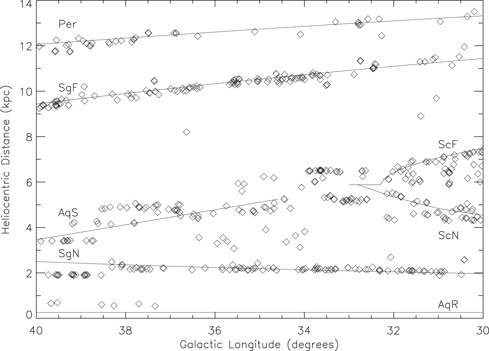
The Hi-GAL compact source catalog provided additional information about the near/far association for a subset of our YB sample. The Hi-GAL distances were assigned by extracting 12CO or 13CO spectra along the line of sight to every Hi-GAL source to determine the VLSR and subsequently employing the Galactic rotation model of Brand & Blitz (1993). In the Hi-GAL catalog, three types of flags are used to indicate the quality of the solution to the near/far distance ambiguity (EMS17). An entry of "G" indicates that the ambiguity was solved by matching the source position with a catalog of sources with known distances (e.g., H ii regions, masers, etc.) or features in extinction maps. If none of these were available, the ambiguity was arbitrarily solved in favor of the far distance, and a bad-quality ("B") flag was assigned. If a distance estimate was unavailable, a null value ("N") was assigned. When a YB was associated with a Hi-GAL source that had a "G" designation, we assigned this Hi-GAL near/far association to the YB while using the Bayesian distance calculator. For example, if a Hi-GAL source had a near distance, then we would set Pfar = 0. For two of the sources (YB 1166 and 1204), the Bayesian distance calculator and the Hi-GAL near/far solution would not agree due to details of the Galactic model, and we adopted the Pfar = 0.5 Bayesian distance. For sources that had a "B" or null flag, we used the Pfar = 0.5 Bayesian distance. The distribution of our sources in the Galactic plane is shown in Figure 1. As expected, there are noticeable source groupings along the spiral arm tracers (e.g., the SgN arm at ∼2 kpc), consistent with the weighting that the Reid et al. (2016) technique gives to the underlying spiral arm structure model.
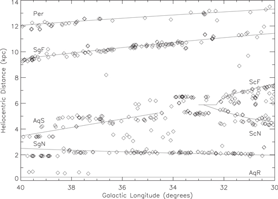
Figure 1. The YB spatial distribution. Heliocentric distances and Galactic longitudes are plotted for all 493 YBs in the pilot region with CO associations (diamonds). The average statistical uncertainty in the distance is ∼0.5 kpc. Lines show the spiral arm tracers along this line of sight from Reid et al. (2016): Per = Perseus, SgN and SgF = Sagittarius near and far sections, ScN and ScF = Scutum near and far sections, AqR = the local Aquila Rift feature, and AqS = the Aquila spur between SgN and ScN.
Download figure:
Standard image High-resolution imageThe assigned distances to YBs with Hi-GAL associations are provided in column (4) of Table 4; for comparison, the kinematic distances reported in the Hi-GAL compact source catalog are also given in column (6). Variations between our distances and those presented in EMS17 can be attributed to the fact that (1) the Bayesian model used additional information beyond a kinematic model to calculate distances and (2) if EMS17 could not resolve the near/far ambiguity, they assumed the far distance, whereas the Reid et al. (2016) distance calculator uses a Bayesian approach to resolve the ambiguity.
Table 4. Physical Properties of YB–Hi-GAL Matched Sources
| YB | l | b | Distance | σd | Hi-GAL Distance | Hi-GAL Dist. Flag |
|---|---|---|---|---|---|---|
| Number | (deg) | (deg) | (kpc) | (kpc) | (kpc) | (G/B/N) |
| (1) | (2) | (3) | (4) | (5) | (6) | (7) |
| 1153 | 30.0033 | −0.2659 | 7.43 | 0.61 | 8.187 | B |
| 1154 | 30.0233 | −0.0429 | 6.70 | 1.49 | 8.976 | B |
| 1155 | 30.0243 | 0.1085 | 7.32 | 0.62 | 7.840 | B |
| 1156 | 30.0325 | 0.1079 | 7.31 | 0.62 | 7.829 | B |
| 1158 | 30.0670 | 0.0976 | 6.00 | 0.96 | 1.000 | N |
| 1159 | 30.0955 | 0.0441 | 7.32 | 0.63 | 7.923 | B |
| 1161 | 30.1320 | −0.6587 | 4.48 | 0.28 | 4.963 | G |
| 1162 | 30.1971 | 0.3085 | 13.5 | 0.35 | 14.156 | B |
| Rescaled Mass | σM | Rescaled LBOL | σL | Rescaled Diameter | σD | |
|---|---|---|---|---|---|---|
| (M⊙) | (M⊙) | (L⊙) | (L⊙) | (pc) | (pc) | |
| (1) | (2) | (3) | (4) | (5) | (6) | |
| 1726.85 | 327.18 | 8055.78 | 1322.75 | 0.49 | 0.04 | |
| 110.71 | 120.19 | 11,118.11 | 5422.01 | 0.51 | 0.11 | |
| 916.74 | 202.75 | 12,669.02 | 2146.12 | 0.65 | 0.06 | |
| 1010.23 | 326.74 | 6279.24 | 1065.15 | 0.66 | 0.06 | |
| 261.36 | 85.26 | 2995.92 | 958.69 | 0.40 | 0.06 | |
| 714.58 | 174.29 | 2504.42 | 431.09 | 0.63 | 0.05 | |
| 116.99 | 114.08 | 461.02 | 108.73 | 0.61 | 0.04 | |
| 2034.84 | 114.10 | 20,209.16 | 1047.88 | 0.71 | 0.02 |
| Lbol/Mass | σL/M | Tgray a |

| Lratio b |

| Tbol c |

| Surface Density (Σ) | σΣ |
|---|---|---|---|---|---|---|---|---|---|
| (L⊙/M⊙) | (L⊙/M⊙) | (K) | (K) | (K) | (K) | (g cm−2) | (g cm−2) | ||
| (1) | (2) | (3) | (4) | (5) | (6) | (7) | (8) | (9) | (10) |
| 4.67 | 1.17 | 15.59 | 0.24 | 59.87 | 11.97 | 45.59 | 9.12 | 1.886 | 0.36 |
| 100.42 | 119.52 | 36.44 | 3.56 | 236.91 | 47.38 | 42.53 | 8.51 | 0.112 | 0.12 |
| 13.82 | 3.85 | 17.08 | 0.66 | 139.1 | 27.82 | 60.22 | 12.04 | 0.584 | 0.13 |
| 6.22 | 2.27 | 16.18 | 0.96 | 70.86 | 14.17 | 53.33 | 10.67 | 0.616 | 0.2 |
| 11.46 | 5.24 | 18.62 | 0.34 | 95.11 | 19.02 | 44.64 | 8.93 | 0.443 | 0.14 |
| 3.5 | 1.05 | 14.34 | 0.48 | 53.44 | 10.69 | 49.33 | 9.87 | 0.485 | 0.12 |
| 3.94 | 3.95 | 16.00 | 0.72 | 45.65 | 9.13 | 40.26 | 8.05 | 0.083 | 0.08 |
| 9.93 | 0.76 | 19.22 | 0.19 | 78.23 | 15.65 | 47.19 | 9.44 | 1.083 | 0.06 |
Notes.
a Dust temperature calculated using graybody fit. b Ratio of Lbol to luminosity calculated for λ ≥ 350 μm. c Bolometric temperature calculated using Equation (5) in EMS17.Only a portion of this table is shown here to demonstrate its form and content. A machine-readable version of the full table is available.
Download table as: DataTypeset image
3.3. Clump Physical Properties
In this section, we examine the properties of the YBs that have associations with EMS17 Hi-GAL compact sources/clumps (see Section 3.1 for details on the catalog cross-match procedure). These sources are of particular interest, as they are the subset of YBs most likely to be associated with star formation activity across a range of both intermediate and high masses. We omit 17 of the 385 YB–Hi-GAL matched sources, as they do not have a 13CO association and related distance measurement. Data for the remaining 368 YB–Hi-GAL sources are shown in Table 4. Columns (1)–(3) give the YB identification and positional information, and columns (4)–(7) give distance-related data as discussed in Section 3.2. Columns (8)–(13) give the EMS17 mass, bolometric luminosity, and diameter rescaled using the distance in column (4). Columns (14)–(23) give distance-independent quantities calculated by EMS17.
We calculated the mass uncertainty (column (9)) by combining the uncertainty in the mass (DMASS) listed in EMS17 and our distance uncertainty in column (5). The Hi-GAL masses were derived as SED fit parameters, and the uncertainty (DMASS) is the larger of ∣M − Mlow∣ and ∣M − Mhigh∣, where M is the best-fit mass, and Mlow and Mhigh are the minimum and maximum mass estimates associated with an acceptable SED fit (D. Elia 2020, personal communication). Two different SED fitting techniques (denoted "thick" and "thin") were used by EMS17. In the majority of the thin fits, the clump mass was not highly constrained by the SED fit (e.g., YB 1154 and YB 1161); in such cases, the masses are essentially known to within a factor of 2.
The bolometric luminosity uncertainty (column (11)) arises from uncertainties in the SED integration and source distance. Roughly the maximum uncertainty in the SED integration is thought to be ∼20% (D. Elia 2020, personal communication). For sources with a poor SED, which we defined as those having a relative mass uncertainty >0.75, we combined a 20% error with our distance uncertainty. For other sources, we only report the uncertainty associated with our distance estimate.
The remaining uncertainties listed in Table 4 are more straightforward to explain. The rescaled diameter uncertainty in column (13) reflects our distance uncertainty. The L/M uncertainty was calculated by propagating the rescaled mass and bolometric luminosity uncertainties from columns (9) and (11). The Tgray uncertainty in column (17) was listed in EMS17 and is repeated here. As both the Lratio and Tbol quantities involve the integration of SEDs, we report a 20% uncertainty as a conservative error estimate. Finally, the surface density error reflects the relative mass uncertainty.
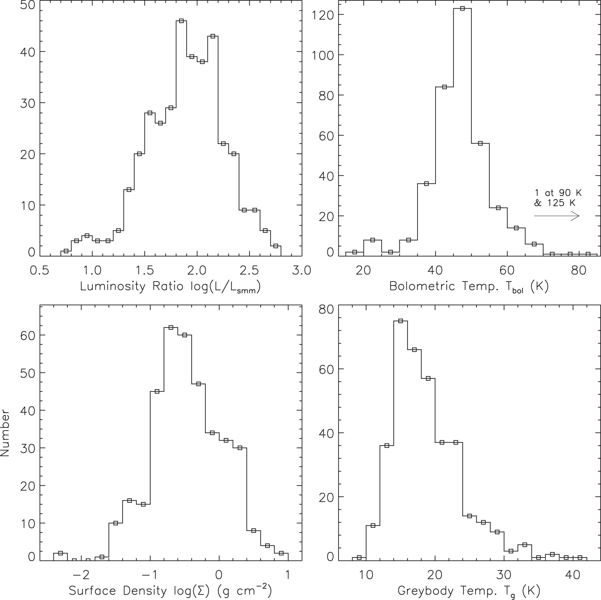
Descriptive statistics for the clump properties are given in Table 5, and histograms of the quantities are shown in Figures 2 and 3. We note that the diameter reported in Table 4 more closely represents the size of the star-forming region containing the YB and may overestimate the size of the YB itself. We address the issue of YB size in more detail in Sections 3.5 and 4.3.
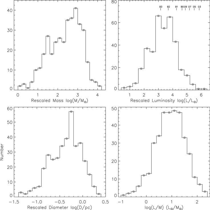
Figure 2. Physical properties of the YB–Hi-GAL matched sources. The lower left and upper row histograms show physical properties from the EMS17 catalog rescaled using our newly calculated distances. For reference, main-sequence OB star luminosities (Crowther 2005) are indicated in the upper right panel. The lower right histogram displays the distance-independent luminosity–mass ratio, also from EMS17. See text for full discussion.
Download figure:
Standard image High-resolution image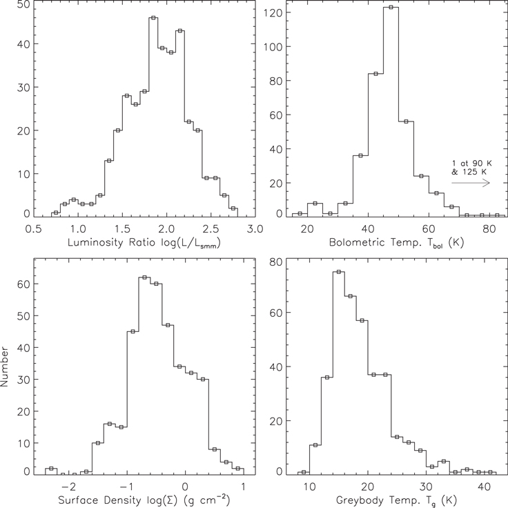
Figure 3. Same as Figure 2. All quantities plotted are distance-independent.
Download figure:
Standard image High-resolution imageTable 5. Descriptive Statistics for the YB–Hi-GAL Matched Sources
| Rescaled Mass | Rescaled Luminosity | Rescaled Diameter | |
|---|---|---|---|

|

|

| |
| Median | 2.51 | 3.33 | −0.32 |
| Mean | 2.37 | 3.30 | −0.37 |
| SD | 0.80 | 0.93 | 0.33 |
| Max. | 4.20 | 6.05 | 0.33 |
| Min. | 0.08 | 0.53 | −1.30 |
| Lbol/Mass | Tgray | Lratio | Tbol | Surface Density | |
|---|---|---|---|---|---|

| (K) |

| (K) |

| |
| Median | 0.96 | 17.8 | 1.91 | 47.0 | −0.49 |
| Mean | 0.93 | 18.8 | 1.89 | 47.2 | −0.46 |
| SD | 0.58 | 5.1 | 0.37 | 9.8 | 0.52 |
| Max. | 2.36 | 40.0 | 2.74 | 127.4 | 0.83 |
| Min. | −1.0 | 8.9 | 0.79 | 18.4 | −2.3 |
Download table as: ASCIITypeset image
The Hi-GAL compact sources were divided into two major groups, prestellar and protostellar, by EMS17. The prestellar sources showed no signs of star formation activity, while the protostellar sources had emission at 70 μm, indicative of embedded star formation activity. As expected, 97% of YB-matched Hi-GAL sources were flagged by EMS17 as protostellar, and we further assume that the remaining Hi-GAL matched YBs are also protostellar because they are emitting in the MIR. Comparison with figures from EMS17 shows that the mass, luminosity, and diameter distributions shown in Figure 2 are all consistent with the properties expected for protostellar objects. This is not unexpected as YBs, by definition, have MIR emission that is likely due to embedded star formation activity. Referring to Figure 2, we see that the YB–Hi-GAL source masses (M) fall mostly in the range  , and the source luminosity (L) falls in the range
  . Most of the YB–Hi-GAL sources have diameters (D) that are in the canonical "clump" range (0.2 pc ≤ D ≤ 3 pc) and thus likely contain multiple sites of star formation. Our diameter distribution is shifted slightly to lower diameters compared to the overall Hi-GAL sample (see Figure 4 in EMS17) and thus includes a larger proportion of "cores" (D < 0.2 pc or
  ). This slight difference may be because of differences in how we resolved the near/far distance ambiguity for sources compared to EMS17. As discussed in Section 3.2, we have assigned a near distance for several sources in our pilot region that EMS17 assumed to be at a far distance.
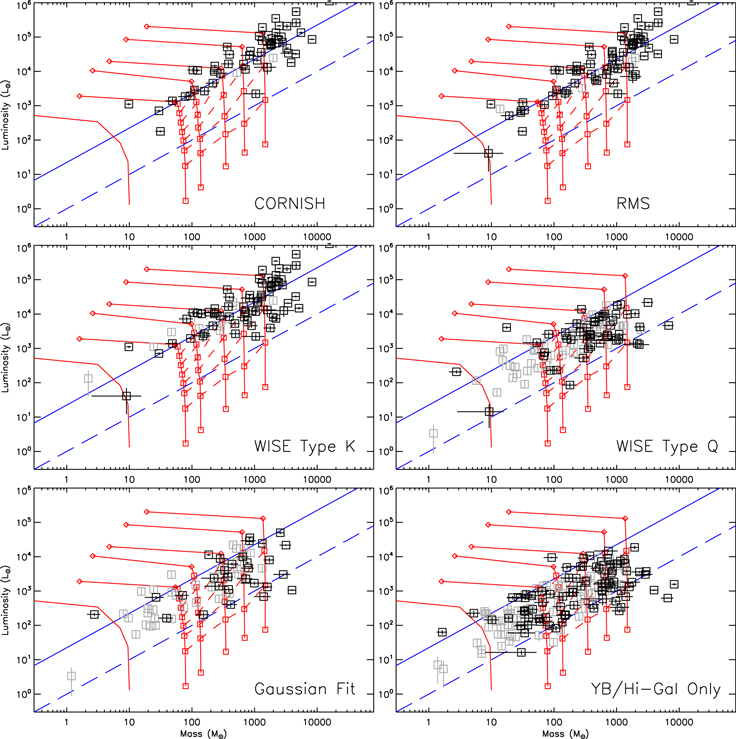
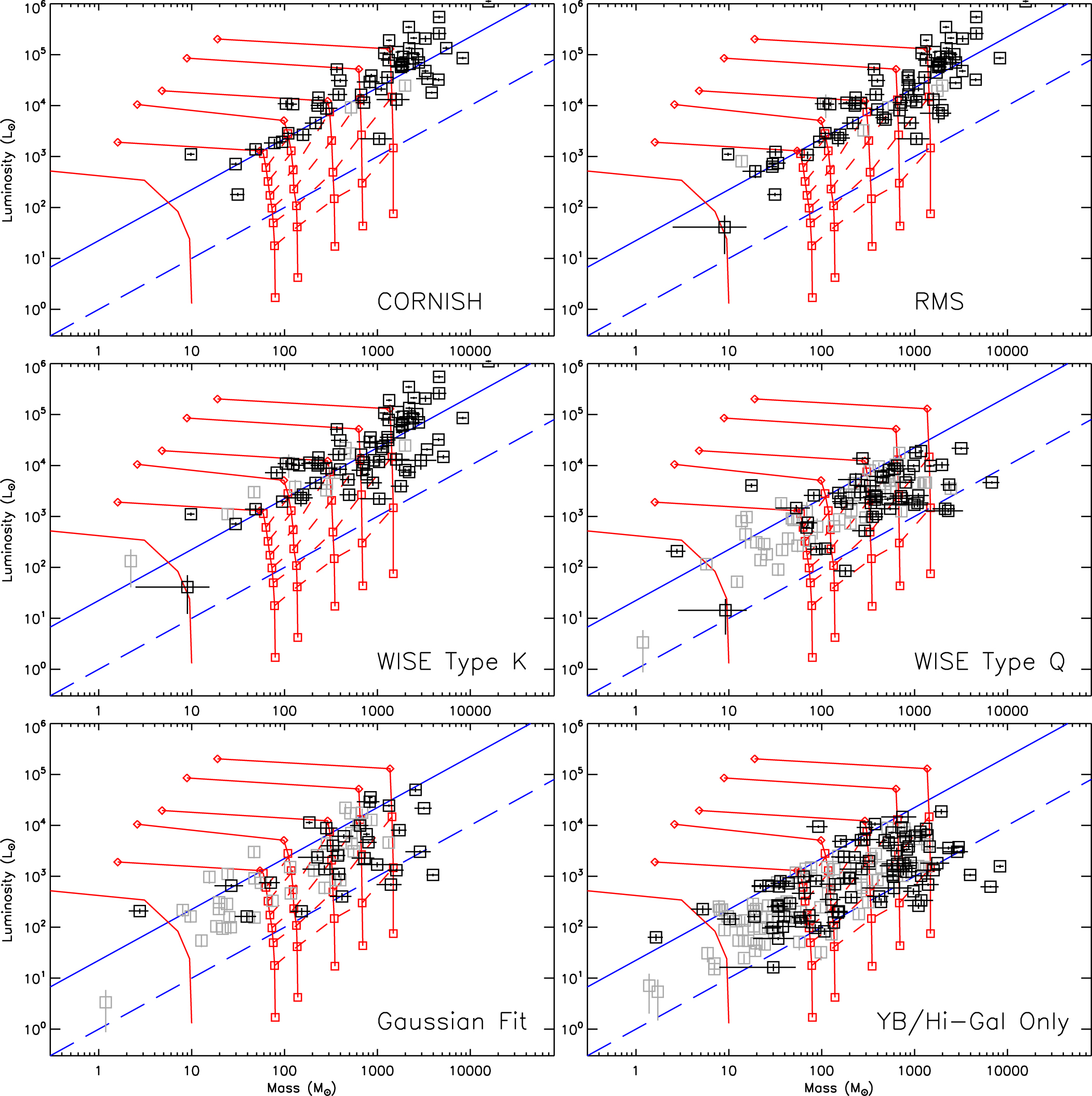
Figure 4. Bolometric luminosity–clump mass plots for various subsets of the YB–Hi-GAL sources. Red lines show the Molinari et al. (2008) clump evolutionary tracks. Small squares along the vertical portion of each track correspond to 5 × 10⁴ yr intervals, and isochrones are the red short dashed lines. The blue upper diagonal line represents a 90th percentile lower limit for Herschel-defined H ii regions, and the blue lower diagonal line is a 90th percentile upper limit for the prestellar objects in the EMS17 sample of Hi-GAL clumps (see text for details). For sources with good SED fits (black), mass and luminosity error bars are shown (most are smaller than the symbol used). Sources with poor SED fits (gray) do not have error bars shown for mass.
Download figure:
Standard image High-resolution imageThe distance-independent quantities provide additional information about the evolutionary stage of the embedded star formation activity, as well as the mass of the forming stellar population. Comparing the lower right panel of Figure 2 with Figure 13 in EMS17, we see that the range of the bolometric luminosity to mass ratio (L/M) is consistent with protostellar sources, but the YB–Hi-GAL peak is shifted to a larger value ( ; cf.
; cf.  ). EMS17 used L/M ≥ 22.4 L⊙/M⊙ (or
  ) to define "H ii region candidates," i.e., compact sources that have embedded high-mass star formation activity. This makes up about 10% of their protostellar sample. In contrast, 24% of the YB–Hi-GAL sources have (L/M) consistent with being H ii region candidates, which is indicative of YBs being associated with a mix of intermediate- and high-mass star formation.
The ratio of the bolometric luminosity to the luminosity in the submillimeter (λ ≥ 350 μm) can be used as a rough proxy for the evolutionary stage of the star formation activity. Regardless of the details of the star formation process, as the source evolves and more stars form within the clump/core, an increasing proportion of the luminosity will originate at shorter wavelengths. Mirroring the criteria used to define low-mass, isolated, class 0 young stellar objects, EMS17 chose  as a representative dividing line between early and more evolved star formation. Comparison of the upper left panel in Figure 3 with Figure 14 in EMS17 shows that while the range of
  is similar to the protostellar sample, the YB–Hi-GAL sample is shifted to the right, with 40% of the YB–Hi-GAL sample having
  compared to only 14% for the full protostellar sample. This shows that the YB–Hi-GAL sample is slightly more evolved than the full Hi-GAL sample.
The bolometric temperature (Tbol), which is defined as the temperature of a blackbody that has the same mean frequency as the observed SED (Myers & Ladd 1993), is another quantity that can easily be related to the evolutionary stage of the object. A cooler Tbol would correspond to earlier stages of star formation where the peak of the SED is shifted to longer wavelengths. Comparing the upper right panel of Figure 3 with Figure 15 in EMS17, we see that the YB–Hi-GAL sources clearly fall in the protostellar range, but there is a deficit of YB–Hi-GAL sources with Tbol < 40 K (only 15% compared to ∼50% for the full sample). This is consistent with the results from the luminosity ratio outlined in the previous paragraph indicating that the YB–Hi-GAL sample is slightly more evolved than the full Hi-GAL sample.
The surface density of a source is often used to identify regions associated with high-mass star formation. A comparison of the lower left panel of Figure 3 with the protostellar sample shown in Figure 7 of EMS17 shows that both distributions have the same peak, around log(Σ) = −0.5, and similar ranges; however, the YB–Hi-GAL distribution is not as symmetric, and it is slightly shifted to higher surface densities. This shift can be quantified by looking at the fraction of sources found above the Krumholz & McKee (2008) threshold for high-mass star formation; 21% of the YB–Hi-GAL sample have Σ > 1 g cm−2, compared with 13% for the full protostellar sample.
Finally, the temperature used in the graybody fits to the Herschel SEDs at λ ≥ 160 μm (Tgray) is shown in the lower right panel of Figure 3. The distribution is similar to the protostellar Tgray distribution shown in Figure 5 of EMS17. The YB–Hi-GAL distribution has a slightly higher average temperature (18.8 K) than the protostellar sample (16.0 K), but it shares approximately the same low-temperature cutoff and high-temperature tail.

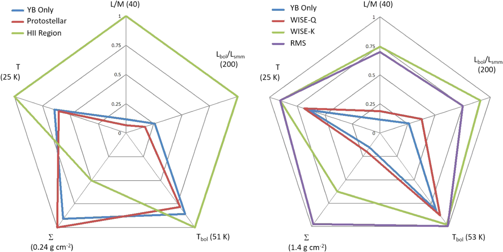
Figure 5. Radar plot visualizations for five distance-independent quantities for different classes of objects. The values plotted are medians, and the maxima are indicated for each radial line. Different classes are connected via different-colored pentagons. In the left panel, protostellar clumps and H ii regions identified in the Hi-GAL survey (EMS17) are compared with YB–Hi-GAL matches lacking counterparts in other surveys. In the right panel, four YB–Hi-GAL subsets are compared. The RMS and WISE K subsets are almost entirely high-mass star-forming regions, while the WISE Q and YB–Hi-GAL-only subsets are a mix of intermediate-mass regions and young high-mass regions.
Download figure:
Standard image High-resolution imageThe comparisons outlined in this section clearly show that the YB–Hi-GAL sources are protostellar objects associated with intermediate- and high-mass star formation spanning a range of evolutionary stages and are more massive and slightly more evolved than the full Hi-GAL sample. In Section 4.1, we combine various observables to learn more about the YB–Hi-GAL sample, and we look at the physical properties of subsets of this sample.
3.4. MIR Photometry
We obtained MIR photometry of YBs at 8.0, 12.0, and 24 μm from our Spitzer and WISE images for 511 of the 516 sources in our pilot region, with five sources omitted due to incomplete image coverage of the source. The Galactic plane exhibits complex, structured backgrounds at MIR wavelengths. Additionally, YBs are typically extended sources, and many YBs that are single, circular features at 12 and 24 μm contain structure like filaments or multiple sources at 8 μm. This is not surprising, due to the higher resolution at 8 μm, and the expectation that young PDRs contain multiple seeds of star formation. Thus, both traditional "stellar" aperture photometry and PSF-fitting photometry are not appropriate techniques. Instead, photometry was done using a program written in Python inspired by the IDL-based imview program (Higgs et al. 1997). Our program allows the user to display an image and interactively select points surrounding the YB that are used to define the local background. The program then interpolates over the area within those points using a multiquadratic radial basis function, creating a background estimate. The difference between the background and image is calculated, resulting in a residual "YB-only" image, and converted to a flux density. Photometry was not conducted for sources that were saturated at 12.0 and/or 24 μm.
The largest source of uncertainty in our flux-density measurements comes from the choice of points used to define the background. To address this uncertainty, three different astronomers conducted the photometry twice for a total of six photometric measurements of each source. We report the mean and fractional error (standard deviation divided by mean) of these measurements in Table 6. We only included sources with a fractional error of <50% in our later analysis in Section 4.2. The Hi-GAL 70 μm photometry results of EMS17 are also included in Table 6 for convenience. Although EMS17 included additional photometry at longer wavelengths, these longer wavelengths become increasingly less likely to be accurately associated with the YBs, so we do not include them here.
Table 6. Pilot Region MIR Photometry
| Source | F8 a |
 a
a
| F12 a |
 a
a
| F24 a |
 a
a
| F70 b | DF70 b | Well Fit by 2D Gaussian Model |
|---|---|---|---|---|---|---|---|---|---|
| (Jy) | (Jy) | (Jy) | (Jy) | (Jy) | |||||
| 1153 | 0.28 | 0.23 | 0.05 | 0.29 | 0.15 | 0.13 | 64.85 | 4.1 | x |
| 1154 | 15.68 | 0.22 | 7.68 | 0.29 | ⋯ | ⋯ | 327.27 | 19.97 | |
| 1155 | 1.36 | 0.29 | 0.67 | 0.13 | 2.96 | 0.11 | 64.34 | 6.5 | |
| 1156 | 0.75 | 0.15 | 0.16 | 0.25 | 1.09 | 0.18 | 46.17 | 1.72 |
Notes.
a We report the mean and fractional error (standard deviation divided by mean) of six separate photometric measurements of each source. See text for details. b Values reported by EMS17.Only a portion of this table is shown here to demonstrate its form and content. A machine-readable version of the full table is available.
Download table as: DataTypeset image
While the basic technique was the same for all three bands, there were some instrument-specific considerations. The IRAC images were in units of megajanskys per steradian, so obtaining the flux density for each source required only a pixel-to-steradian conversion factor of 3.385 × 10⁻¹¹ sr pixel−1 (1 2 pixels; Fazio et al. 2004). The IRAC Instrument Handbook (IRAC 2015) includes plots showing recommended aperture corrections for 8.0 μm photometry of extended sources. The average MWP radius for the DR2 YBs is ∼12'', and, if we take this to be a typical aperture size, an aperture correction of at most 0.85–0.8 should be applied. To simplify the collection of photometry, we chose not to apply any aperture corrections to our data, as the resulting shift in the MIR colors is very small. For example, the largest aperture correction expected (∼0.8) would correspond to a shift in F12/F8 of only 0.1 dex. A source radius may be used to select an aperture correction for the data shown in Table 6; however, this would introduce new uncertainty from ambiguity in the appropriate source radius (see discussion in Section 4.3). The WISE All-Sky Catalog release document (Cutri et al. 2012) lists a WISE 12 μm band aperture correction for extended objects of 0.973. As with the IRAC data, we did not apply the correction. The raw photometry in WISE data numbers (DNs) was converted to janskys using a DN-to-jansky conversion factor of 1.8326 × 10⁻⁶ Jy DN−1, which incorporates recommended zero-point magnitudes and fluxes. Finally, the MIPS instrument handbook (MIPS 2011) did not suggest any aperture corrections for extended sources. MIPS images were in units of megajanskys per steradian, so conversion to flux density involved only the pixel-to-steradian conversion factor of 3.673 × 10⁻¹¹ sr pixel−1 (125 pixels).
3.5. 2D Gaussian Fits
The YBs in the full catalog generated by the MWP DR2 are very heterogeneous, with many showing extended structure and multiple point sources. To isolate compact structures, we fit 2D Gaussians to the YB 8 and 24 μm emission in the background-subtracted, "YB-only" images generated in the photometry process discussed in Section 3.4. We note that while the photometry was repeated six times per source, only one set of background-subtracted images was used for the fitting. To see how well fit the YB-only images were by a 2D Gaussian, we created a residual of 2D Gaussian fits subtracted from the YB-only image, which we refer to as the "residual image" in the rest of this section. We measured the magnitude of the residuals, differences in 8 and 24 μm peak locations, and differences in 8 and 24 μm Gaussian standard deviations. The coincidence of the 8 and 24 μm peaks and comparable spatial extents at these wavelengths are expected features of young PDRs. In order to assess the similarity of the fits at 8 and 24 μm, we defined a series of points. The YBs were given up to four points, one point for fulfilling each of the following criteria.
- 1.The absolute value of the flux in the residual is ≤10% of the flux in the Gaussian fit to the 8 μm image.
- 2.The absolute value of the flux in the residual is ≤10% of the flux in the Gaussian fit to the 24 μm image.
- 3.The distance between the center of the 8 and 24 μm Gaussians is <0.3 times the average of the 8 and 24 μm standard deviations (σ8 μmx + σ8 μmy + σ24 μmx + σ24 μmy)/4.
- 4.The normalized difference between the average of the 8 and 24 μm standard deviations satisfies ∣σ8 μm − σ24μm∣/((σ8μm + σ24 μm)/2) < 0.4.
Each source that gained four points can therefore be considered well fit by a 2D Gaussian model at both 8 and 24 μm. These Gaussian sources are consistent with being compact PDRs or possibly evolved stars; however, our color analyses suggest that YBs are predominantly young sources (see Section 4.2). Ninety-six of the full sample of 516 YBs received four points (18.6%): 65 of these have Hi-GAL clump matches, 9 have only WISE (8Q, 1C) catalog matches, 6 have no associated molecular gas velocities, and 16 lack matches in any catalog. Sources that earned four points are flagged in Table 6. In Section 4.3, we compare the results of our Gaussian fits with MWP YB sizes and the sizes of associated Hi-GAL clumps.
4. Analysis and Discussion
4.1. Properties of YB–Hi-GAL Subsets
In Figure 4, we show bolometric luminosity (L) versus clump, or envelope, mass (M) plots for different subsets of YB–Hi-GAL matched clumps. The position of a clump in an L–M plot is related to its evolutionary stage. In each plot, we show simplified evolutionary tracks based on the Molinari et al. (2008) model for the evolution of star-forming protostellar clumps, and each track corresponds to a star-forming clump with a given initial envelope mass. The vertical portions of each track correspond to when the embedded protostar(s) are forming and rapidly gaining mass from their birth clouds; the luminosity of the cloud increases due to accretion and internal heating from the protostar(s), and the gas mass of the clump is lowered slightly, reflecting primarily the conversion of gas to stars. The subsequent horizontal tracks (between diamonds) correspond to the relatively slower process of cloud dispersal; the luminosity remains roughly constant, reflecting the luminosity of the newly formed stars, while the remaining gas is removed via processes like bipolar outflows, stellar winds, radiation pressure, and photoionization. Small squares along the vertical portion of each line correspond to 5 × 10⁴ yr intervals, and isochrones are indicated using short dashed lines. The upper diagonal line represents a 90th percentile lower limit for H ii regions,  L⊙/M⊙, which was defined by EMS17 using Hi-GAL–CORNISH H ii region matches. The lower diagonal line is a 90th percentile upper limit for the prestellar objects in the EMS17 sample of Hi-GAL clumps,
  L⊙/M⊙.
Not surprisingly, we see that the vast majority of the CORNISH-, RMS-, and known compact H ii region (WISE K)–matched YBs fall primarily along and above the  line. They also tend to be near the vertical–horizontal transition region for the various evolutionary tracks, as would be expected for objects like compact H ii regions, which represent fairly evolved states of massive star evolution. Note that there is significant overlap between these three groups (see Table 2). In contrast, objects that are radio-quiet (WISE Q), well fit by 2D Gaussians, and YBs with only Hi-GAL matches tend to lie along the active accreting portion of the evolutionary tracks for a wide range of clump masses and luminosity. There is also a noticeable deficit of these sources (compared to the CORNISH, RMS, and WISE K samples) in the upper right corner of the L–M plots (M > 103
M⊙, L > 104
L⊙).
line. They also tend to be near the vertical–horizontal transition region for the various evolutionary tracks, as would be expected for objects like compact H ii regions, which represent fairly evolved states of massive star evolution. Note that there is significant overlap between these three groups (see Table 2). In contrast, objects that are radio-quiet (WISE Q), well fit by 2D Gaussians, and YBs with only Hi-GAL matches tend to lie along the active accreting portion of the evolutionary tracks for a wide range of clump masses and luminosity. There is also a noticeable deficit of these sources (compared to the CORNISH, RMS, and WISE K samples) in the upper right corner of the L–M plots (M > 103
M⊙, L > 104
L⊙).
WISE Q sources are particularly interesting, as they are objects that were classified as potential H ii regions based on their infrared colors and morphology, but they lack significant/detectable radio emission (Anderson et al. 2014). Our examination of the L–M plots suggests that a (modest) majority of the WISE Q objects are radio-quiet because they are associated with low- and intermediate-mass star formation. We note that sources associated with clump masses below 500 M⊙ represent about 63% of the sample. If these objects are evolving along the evolutionary tracks shown, they correspond to regions with a final luminosity of <104 M⊙, which, assuming that a single star forms, is the luminosity expected for a single B1 V star. The remaining WISE Q sources (∼37%) are associated with more massive clumps that are still on the vertical portion of their evolutionary tracks. In this case, the lack of radio emission could be because ionizing photons are being absorbed by the dusty envelope surrounding a newly formed massive star or the clump is forming multiple intermediate-mass stars that are unable to form a significant H ii region. We note that this proportion of WISE Q sources associated with high-mass star formation (37%) is much higher than the number given using a Σ > 1 g cm−2 cutoff (5.3%); however, it is comparable to the number found using the Σ > 0.3 g cm−2 cutoff (41%) suggested by López-Sepulcre et al. (2010). For comparison, the fraction of the entire YB–Hi-GAL sample associated with high-mass star formation is 21%, 53%, and 41% using Σ > 1 g cm−2, Σ > 0.3 g cm−2, and a clump mass >500 M⊙, respectively.
The 2D Gaussian well-fit sources, shown in the lower left panel of Figure 4, have a uniform distribution in both clump mass and luminosity. The majority of the sources appear to be in the accretion stage of their evolution. This may be due to the fact that more evolved sources have a more complex infrared morphology formed as material is dispersed.
The YB–Hi-GAL-only sources also have a uniform distribution of clump mass and luminosity, and again, the majority of the sources appear to be in the accretion stage of their evolution. Unlike the other subsets, the YB–Hi-GAL-only sample includes a very large fraction of sources that are associated with lower-mass clumps (45% of sources associated with clumps with M < 102 M⊙).
As discussed in Section 3.3, distance-independent quantities are useful for distinguishing between different evolutionary stages and different masses in star-forming regions. The five quantities we examine are dust temperature (T), bolometric temperature (Tbol), ratio of bolometric luminosity to luminosity calculated over wavelengths longward of 350 μm (Lbol/Lsubmm), ratio of bolometric luminosity to clump mass (Lbol/M), and surface density of the clump (Σ). One way to simultaneously compare these quantities for different samples is through a "radar plot" showing the median values (EMS17).
Figure 5 presents two radar plots of the five distance-independent quantities associated with different subsets of the YB–Hi-GAL sample. In each case, the median of each quantity is plotted along one of five axes. Each axis is normalized to the value indicated at the end of the axis in order to account for the different numerical ranges spanned by each quantity. The left panel compares our YB-only subsample of YB–Hi-GAL sources with the protostellar and H ii region subsamples from EMS17. On average, the YB–Hi-GAL and protostellar samples are very similar, and they are both quite distinct from the H ii region sample. The right panel compares the median values for the different subsets defined in this study. We notice that the WISE K and RMS samples are similar except for the much higher surface density associated with the RMS sample. This likely reflects the more embedded nature of the objects selected for the RMS catalog. If we consider the WISE K and RMS subsets to be essentially all high-mass regions, the position of the WISE Q and YB-only subsets reflects having an increasing proportion of intermediate-mass star-forming regions in the sample; a lower Lbol/M and Σ would be expected. In addition, these subsets could contain a population of less evolved, higher-mass regions, which would have a lower Lbol/Lsubmm and Tbol.
4.2. YB Colors
A significant finding of KWA15 was that the IR colors of YBs, as measured by their fluxes at 8 and 12 μm, might be particularly useful in distinguishing compact PDRs from H ii regions. The PAH emission features around 7–8 and 12 μm are highly sensitive to the PAH ionization state, with the 7–8 μm lines becoming much stronger than the 12 μm lines for ionized PAHs (Roelfsema et al. 1996; Draine & Li 2007). The PAH ionization fraction in a PDR is related to the compactness of the PDR (Roelfsema et al. 1996); a more compact PDR will experience a more intense radiation field, resulting in a higher PAH ionization fraction, stronger emission around 7–8 μm, and a lower log(F12/F8) color. On average, YB PDRs are more compact than typical H ii regions, thus causing the color shift to lower log(F12/F8) colors. It was concluded by KWA15 that a higher fraction of compact objects with a large PAH ionization fraction leads to increasingly negative log(F12/F8) values.
Out of 516 YBs in our pilot region, 434, 361, and 351 had 8, 12, and 24 μm photometry results with repeated measurements yielding a fractional error of <0.5 and were thus deemed "reliable," as discussed in Section 3.4. We extend the KWA15 analysis to the larger DR2 sample and examine YB colors using additional IR wavelengths. The histogram of the log(F12/F8) results for DR2, similar to that shown in KWA15, is shown in Figure 6.
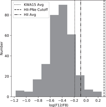
Figure 6. Distribution of the  colors for the 324 YBs in our pilot region with reliable 8 and 12 μm photometry. The dotted line is the average color from KWA15, the dotted–dashed line is the average color of H ii regions from Anderson et al. (2012), and the dashed line is the color separation H ii region–PNe cutoff from Anderson et al. (2012).
Download figure:
Standard image High-resolution imageIt was found by KWA15 that the average value of their sample (−0.19) was more negative than the average color sample of WISE H ii regions (−0.09; Anderson et al. 2012) and that the YBs in their sample without RMS counterparts had an even more negative average of −0.23. The colors of our new YB sample yield an even more negative mean log(F12/F8) value of −0.43 ± 0.15. Size measurements (based on MWP user radii) confirm that our new YB sample indeed contains a larger number of very compact sources. Whereas the mean (± standard deviation) diameter of the RMS-matched YBs with distances from KWA15 is 0.94 ± 0.71 pc, the mean diameter of all YBs with good distance estimates in our current sample is 0.75 ± 0.53 pc. The median diameters are smaller (0.77 and 0.63 pc, respectively), as relatively few YBs are significantly larger than 1 pc. The mean diameter of the subset of YBs with counterparts in catalogs of H ii regions and MYSOs (CORNISH, RMS, WISE C, G, K) is 0.96 ± 0.62 pc, and the mean (± standard deviation) log(F12/F8) color of these objects is −0.28 ± 0.31; however, the mean diameter of YBs lacking such counterparts is 0.65 ± 0.45 pc, and the mean log(F12/F8) color of this subset is −0.47 ± 0.24. Many compact YBs were missed in the KWA15 sample, which was drawn from images at lower zoom levels, where citizen scientists would have been more likely to notice large and bright YBs. Additionally, only YBs with RMS counterparts had associated distances in the KWA15 sample; our current sample indicates that YBs with counterparts in catalogs of H ii regions and MYSOs are biased to physically larger objects.
In addition to measurements at 8 and 12 μm, we use longer MIR wavelengths at 24 and 70 μm to examine the YB population in our DR2 sample. We show an MIR color–color plot in Figure 7 for the 219 YBs in our pilot region with reliable 8 and 24 μm photometry, as well as counterparts in the Hi-GAL survey (EMS17). The color–color plot indicates sources with cross-matches in the RMS and WISE catalogs. The average H ii region colors and H ii region–planetary nebulae (PNe) cutoff colors established by Anderson et al. (2012) are also indicated in Figure 7. WISE sources were separated into categories by Anderson et al. (2014): "K" for known, "G" for group, "C" for candidate, and "Q" for radio-quiet. The YBs with counterparts in the RMS catalog and/or WISE K, G, and C sources are, unsurprisingly, grouped near the expected colors for H ii regions. We find a significant number of sources with WISE Q (n = 44) or no counterpart (n = 101). These WISE Q and no-association sources are predominantly clustered in a separate region of the color–color plot than the WISE K, G, and C and RMS sources, with colors brighter at both 8 and 70 μm than they are at 24 μm. A possible interpretation of this distribution (similar to that described by Chan & Fich 1995 for 12/25/60 μm observations of H ii regions) is that the log(F24/F8) color acts as a measure of the hardness of the incident ultraviolet (UV) radiation field, where a hard UV field, with abundant photons beyond the Lyman limit, would destroy PAH 8 μm emitters, and a softer UV field would excite the PAHs without destroying them (Desert et al. 1990; Giard et al. 1994). Thus, a low log(F24/F8) value may indicate a region with a soft UV field consistent with environments of intermediate-mass stars. The log(F70/F24) axis may measure dust temperature, where emission from a cooler environment would peak at longer wavelengths. Consequently, the region traced by the WISE Q and no-association YBs is consistent with their being cooler and lower in mass than the YBs in the upper left of Figure 7.
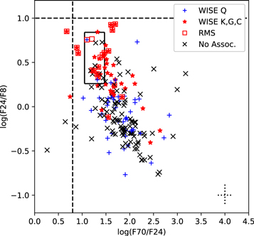
Figure 7. Color–color plot of the 219 YBs in our pilot region with reliable 8 and 24 μm photometry and Hi-GAL counterparts. The 8 and 24 μm photometry is described in Section 3.4. The 70 μm photometry is from EMS17. The colors and shapes indicate the YB association with objects in other catalogs using cross-matching as described in Section 3.1. The solid square indicates the region of mean colors of H ii regions established by Anderson et al. (2012), while vertical and horizontal dashed lines indicate the Anderson et al. (2012) IR color cutoffs for distinguishing H ii regions from PNe. The dotted lines in the lower right corner indicate the average uncertainty in the reported values.
Download figure:
Standard image High-resolution imageWe have shown that, on average, YBs with CORNISH, RMS, and WISE C, G, K matches are larger than those lacking counterparts with either H ii regions or MYSOs (∼1 pc versus ∼0.7 pc). They are also more luminous (see Section 4.1) and have higher log(F12/F8) colors (∼−0.3 versus ∼−0.5) and log(F24/F8) colors (see Figure 7). In addition to distinguishing YBs by mass, is it possible to distinguish evolutionary sequences using MIR colors?
If we assume that a smaller YB is also younger, we can distinguish the youngest YBs by examining only compact YBs, which we define as those with MWP user diameters less than 0.3 pc. There are only 14 compact YBs that have H ii region or MYSO matches and reliable colors at 8 and 12 μm. These sources have log(F12/F8) = −0.42 ± 0.22, more negative than the full massive YB sample. The 47 compact YBs with only WISE Q or no associations do not show significantly different log(F12/F8) colors than their larger counterparts, with log (F12/F8) = −0.52 ± 0.24. All of these results support the expectation that MYSOs rapidly evolve to H ii regions (see isochrones in Figure 4). This preliminary analysis is encouraging but limited by a small sample size. Photometry results for the full DR2 catalog will enable us to better distinguish the mass and evolutionary stages of YBs.
4.3. Measuring YB Sizes
Is a radius measured by MWP users an accurate representation of YB size? The YBs emit radiation across a broad range of wavelengths, and the different wavelengths may trace different extents of a clump and also be observed with different resolution limits. Thus, it is not clear how to define the "size" of a YB. For determining the far-IR fluxes of YBs, we utilized their association with Hi-GAL clumps, whose diameters are based on beam-deconvolved 250 μm Herschel data (EMS17); however, user-measured MWP sizes of YBs are based on their compact "yellow" appearance in combined 24–8–4.5 μm Spitzer RGB images. Along with the 2D Gaussian fits (see Section 3.5), we have three independent measures of size. For any given YB, there can be significant variation between the different measures employed to estimate YB size. For example, differences in MWP and Gaussian sizes can be greatly affected by a given object's location within a complex background.
Figure 8 presents a scatter plot comparing the angular radii of YBs as measured by MWP users to 2D Gaussian standard deviations. This plot indicates that there is a strong correlation between MWP radii and YB sizes as measured by the 2D Gaussian fits to the 8 and 24 μm images. The correlation is even stronger when only well-fit YBs—those that satisfy the four-point criteria detailed in Section 3.5—are considered. Although the error bars on user measurements are large, Pearson's correlation coefficient (r) for the 450 unsaturated YBs plotted in the upper panel is 0.73. The error bars are smaller for the subset of 89 well-fit YBs, and the correlation coefficient is 0.81, indicating that the probability that these two parameters are uncorrelated is essentially zero. The slope of the linear fit to the full sample is 1.4 (1.5 to the well-fit subset). This indicates that, on average, sizes measured by MWP users are proportional to YB sizes determined from 2D Gaussian fits to the 8 and 24 μm emission.
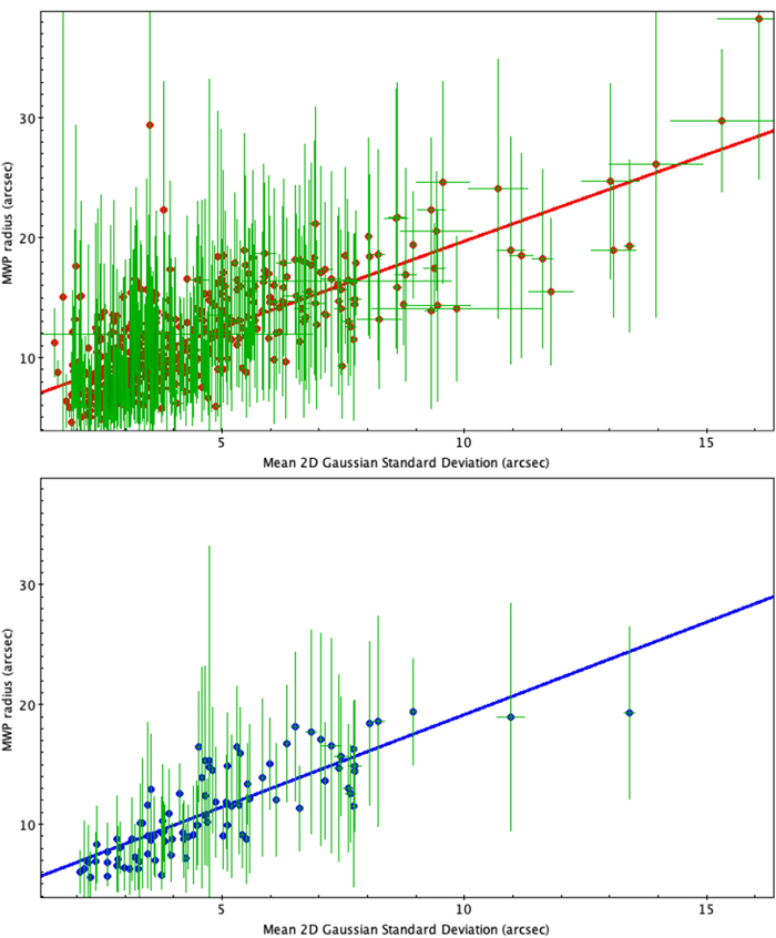
Figure 8. The MWP radius vs. mean 2D Gaussian standard deviation for unsaturated YBs. Top panel: 450 YBs (red symbols and linear fit). Bottom panel: subset of 89 well-fit YBs (blue symbols and linear fits). Error bars are shown in green. Many of the errors on the Gaussian standard deviations are too small to be visible.
Download figure:
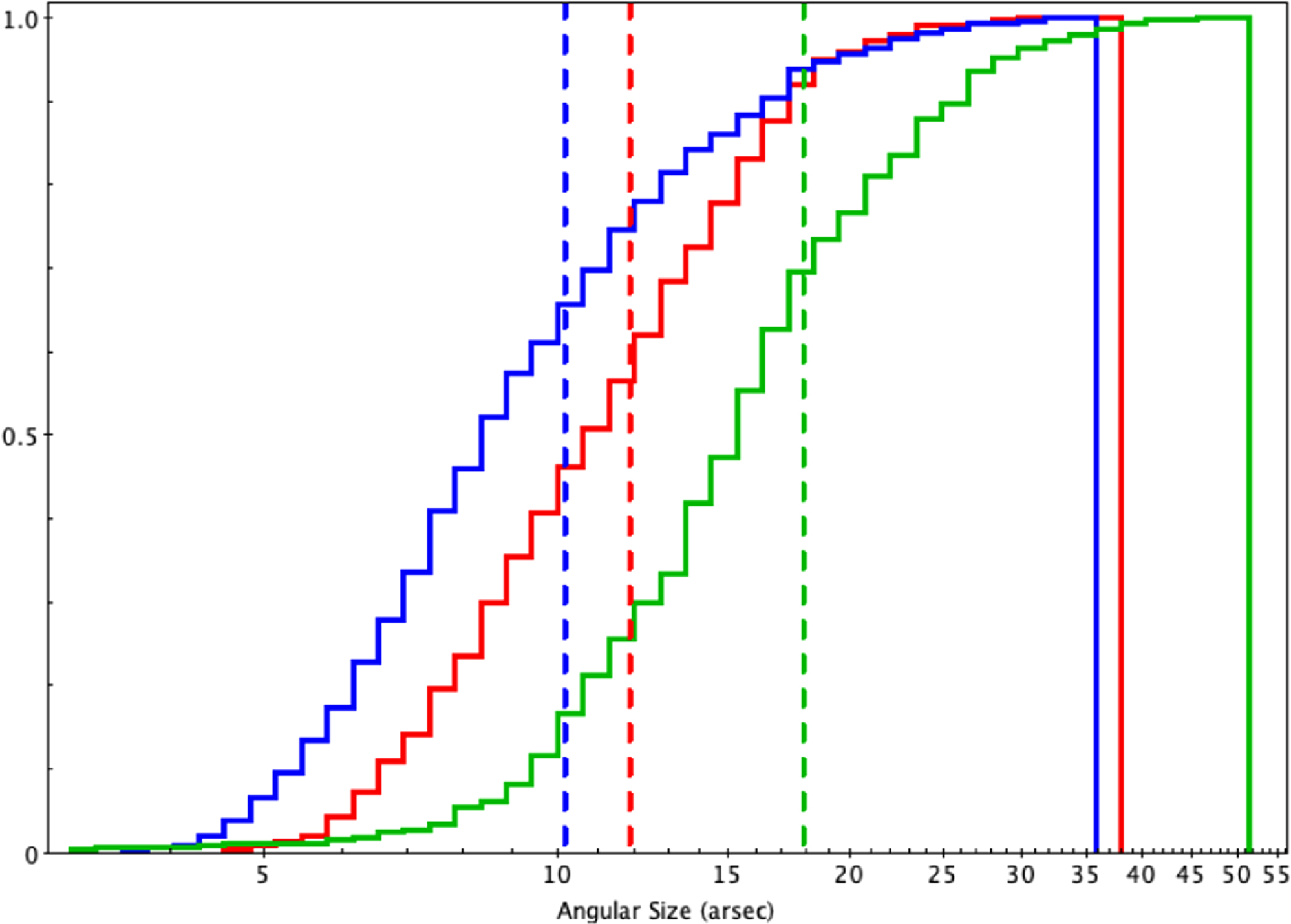
Standard image High-resolution imageFigure 9 presents normalized histograms of the cumulative angular size distributions for MWP radii, 2D Gaussian FWHM (2.355σ), and beam-deconvolved Hi-GAL 250 μm FWHM. Average angular sizes for each distribution are indicated by dashed vertical lines of the same color as the corresponding histogram. The average user-measured MWP radius (119 ± 45) is comparable to the average 2D Gaussian FWHM (102 ± 52), while the average beam-deconvolved 250 μm FWHM is somewhat larger (179 ± 73). The larger size at 250 μm probably reflects a combination of factors, including lower resolution and the likelihood that compact PDRs are still contained within their birth clumps. We conclude that MWP user radii appear to be proportional to 2D Gaussian FWHM, such that trends (i.e., which sources are largest versus smallest) are consistent across both measures of size.
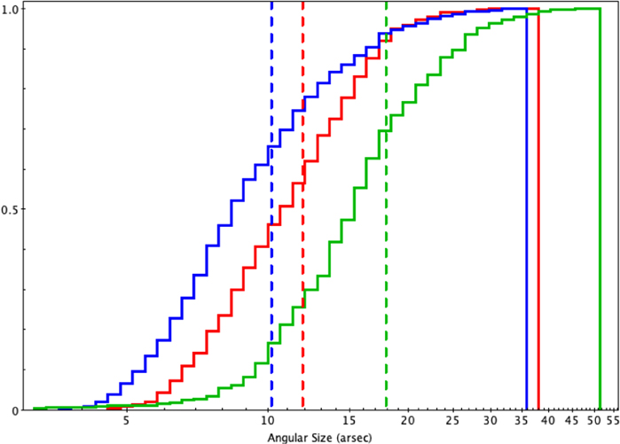
Figure 9. Normalized cumulative histograms for user-measured MWP radii (red), 2D Gaussian FWHM (blue), and Hi-GAL 250 μm FWHM (green) YB size distributions. Dashed vertical lines indicate the mean angular sizes for each distribution using the same colors.
Download figure:
Standard image High-resolution image5. Conclusions
We return once more to the question posed by KWA15, "What are YBs?" Our work supports the main conclusion of KWA15: YBs appear to occupy a transitional phase of massive and intermediate-mass star formation, when a compact PDR has formed around an embedded protostar and the surrounding interstellar medium remains relatively undisturbed. This paper expands on KWA15 by measuring the physical properties of YBs. We find that a "typical" YB is subparsec in size and has physical properties consistent with being a B-type protostar, but YBs are a heterogeneous sample of objects that span a wide range of mass and evolutionary stage. The percentage of YBs that represents massive versus intermediate-mass star formation varies with the method used to probe YB properties. The properties of the YBs in our pilot region are summarized as follows.
- 1.Of the YBs, 30% have spatial cross-matches with at least one tracer of massive star formation in the CORNISH, RMS, or WISE (C, K, and G sources) catalogs (Section 3.1). This is lower than the number of YB cross-matches with tracers of high-mass star formation reported in KWA15 and reflects the larger number of lower-mass YBs identified in MWP DR2. We expect a significant fraction of these to be precursors to optically revealed Herbig Ae/Be nebulae.
- 2.The YBs span several orders of magnitude in luminosity and are embedded in dense clumps that likewise span several orders of magnitude in mass. The mass and luminosity ranges are consistent with the clumps being sites of intermediate and massive star formation. The masses are in the range
 , and the luminosities are in the range , with a mean of 2.37 M☉ and mean of 3.30. Clumps containing YBs are more massive and luminous than the protostellar clumps in the full Hi-GAL catalog (Section 3.3).
 - 3.Approximately 24% of clumps containing YBs have L/M consistent with being H ii region candidates (Section 3.3).
- 4.
- 5.The YB bolometric luminosities and temperatures indicate that the YB sample is slightly more evolved than the full protostellar sample measured by the Hi-GAL catalog (Section 3.3).
- 6.The YBs have very heterogeneous structures, especially at shorter MIR wavelengths, and a majority are not well fit by 2D Gaussian models (Section 3.5). In particular, evidence of multiple sources visible only in the 8 μm images of YBs indicates that many YBs may be compact PDRs encompassing multiple low- and/or high-mass stellar embryos or hypercompact, ultracompact, or compact H ii regions (Motte et al. 2018).
- 7.A large proportion of YB–WISE Q sources (∼37%) are likely associated with massive star-forming regions at a young, radio-quiet evolutionary stage. The remaining ∼63% of YB–WISE Q sources are associated with regions of intermediate-mass star formation (Section 4.1).
- 8.The MIR colors of YBs indicate that many of them are highly compact, with a large PAH ionization fraction. Of the 219 sources in our pilot region with reliable 8 and 24 μm photometry and Hi-GAL counterparts, 46% of the sources have no counterpart in the WISE, CORNISH, or RMS catalogs and 20% have WISE Q counterparts. These sources have MIR colors consistent with being lower-mass and cooler sources than the YBs that have CORNISH, RMS, and/or WISE K, G, or C counterparts (Section 4.2).
- 9.While the size measurement of a YB depends on wavelength and is complicated by resolution limits, MWP user measurements reasonably trace the extents of YB PDRs (Section 4.3). The MWP user measurements, 2D Gaussian fits, and distance-rescaled Hi-GAL clump diameters (Section 3.3) indicate that the majority of YBs have subparsec diameters and are typically embedded in subparsec clumps.


The above evidence suggests that ≳20% of YBs contain high-mass star formation and could go on to produce expanding H ii regions that produce MIR bubbles; thus, we expect that ≳100 of the YBs in this region will eventually go on to become bubbles. The accretion phase of a massive protostar should be on the order of ∼105 yr, while the lifetime of an expanding H ii region should be on the order of ∼106 yr (Motte et al. 2018). Therefore, we would expect a roughly 10:1 ratio of bubbles to massive YBs. The MWP DR2 catalogs (Jayasinghe et al. 2019) identified an ∼1:2 ratio of bubbles to YBs in our pilot region, and this ratio becomes ∼4:1 when only massive YBs are considered. We note that the bubble catalog of Jayasinghe et al. (2019) has been more rigorously culled of possible false detections, whereas our catalog contains all YBs identified by MWP users, which may partially account for the apparent remaining overcount of YBs compared to bubbles.
Many of the intermediate-mass YBs do not have existing catalogs of their physical properties and colors. Thus, this YB pilot region study and future full YB catalog provide a valuable new data set of properties for intermediate-mass star-forming regions. We will expand the work from this pilot region of 516 YBs to the full catalog of over 6000 YBs.
The authors wish to thank Davide Elia for a useful discussion of error estimates for quantities in the Hi-GAL compact source catalog. This publication uses data generated via the Zooniverse.org platform, development of which is funded by generous support, including a Global Impact Award from Google and a grant from the Alfred P. Sloan Foundation. This research has made use of the VizieR catalog access tool, CDS, Strasbourg, France (DOI: 10.26093/cds/vizier); Astropy, 8 a community-developed core Python package for astronomy (Astropy Collaboration et al. 2013; Price-Whelan et al. 2018); data products from the Wide-field Infrared Survey Explorer, which is a joint project of the University of California, Los Angeles, and the Jet Propulsion Laboratory/California Institute of Technology, funded by the National Aeronautics and Space Administration; NASA's Astrophysics Data System Bibliographic Services; and observations made with the Spitzer Space Telescope, which was operated by the Jet Propulsion Laboratory, California Institute of Technology, under a contract with NASA. K.D., A.P., J.M., L.T., A.C., and S.S. were supported during work on this project by the Murdock Charitable Trust under grant No. NS-2016246. G.W.C. was supported in part by a Research Seed Grant through the Illinois Space Grant Consortium. The authors thank the numerous MWP volunteers whose efforts made the DR2 data set possible, and the anonymous referee whose feedback helped to improve this paper.
Software: Astropy (Astropy Collaboration et al. 2013; Price-Whelan et al. 2018), Matplotlib (Hunter 2007), TOPCAT (Taylor 2005).