


Abstract
Magnetohydrodynamic (MHD) turbulence plays an important role for the fast energy release and wave structures related to coronal mass ejections (CMEs). The CME plasma has been observed to be strongly heated during solar eruptions, but the heating mechanism is not understood. In this paper, we focus on the hot, dense region at the bottom of the CME and the generation of coronal wave trains therein using a high-resolution 2.5D MHD simulation. Our results show that the interaction between the tearing current sheet and the turbulence, including the termination shocks (TSs) at the bottom of the CME, can make a significant contribution to heating the CME, and the heating rate in this region is found to be greater than the kinetic energy transfer rate. Also, the turbulence can be somewhat amplified by the TSs. The compression ratio of the TS under the CME can exceed 4 due to thermal conduction, but such a strong TS is hardly detectable in all Solar Dynamics Observatory/Atmospheric Imaging Assembly bands. And turbulence is an indispensable source for the periodic generation of coronal wave trains around the CME.
Export citation and abstract BibTeX RIS
1. Introduction
Coronal mass ejections (CMEs) are the largest explosions in the solar system, where of order of 1029–1032 erg of magnetic energy is released through magnetic reconnection (Forbes 2000). Usually, a flare arcade is formed underneath, attached to the CME by a long, thin current sheet (CS). The propagation speeds of CMEs vary over a wide range from less than 20 km s−1 up to 2000 km s−1, and a fast enough magnetic reconnection rate is required to support a successful eruption (Lin 2002). Magnetohydrodynamic (MHD) turbulence is important for the rapid energy release by introducing multiple reconnection sites in the process of solar eruptions (Lin et al. 2007; Loureiro et al. 2007). And the turbulence must give rise to energy cascading from large to small scales (Lazarian et al. 2020). A tearing instability occurs in the CS to generate copious plasmoids, and it facilitates the various types of reconnection taking place simultaneously, when the Lundquist number of the CS exceeds the value of S ≈ 104 (Bárta et al. 2011; Shen et al. 2011; Mei et al. 2012). Nishida et al. (2009, 2013) demonstrated that the ejected small-scale plasmoids could locally increase the reconnection rate intermittently in both 2D and 3D simulations. As the turbulence fully develops in the nonlinear regime, the reconnection rate is almost independent of the initial configuration and the Lundquist number (Bhattacharjee et al. 2009).
The reconnection outflows and plasmoids can interact with the top of the flare loops to drive oscillations and additional energy release, which might be related to the formation of the supra-arcade fans above the loop top (Hanneman & Reeves 2014; Innes et al. 2014; Cai et al. 2019; Ye et al. 2020) and intermittency in the hard X-ray (HXR; Nishizuka et al. 2009). The oscillation in this region is argued to be full of fast-mode magnetoacoustic waves (Takasao & Shibata 2016) or driven by the Kelvin–Helmholtz instability (Fang et al. 2016; Ruan et al. 2018). Recent spectroscopic observations for the X-8.2 class solar flare on 2017 September 10 gave direct evidence that fractal and turbulent reconnection proceeds efficiently in the CS (Cheng et al. 2018; Li et al. 2018), and substantial plasma heating and major particle acceleration spots are found at the top of the flare arcade (Warren et al. 2018; Chen et al. 2020).
However, due to the limits of the resolution of the observational instruments, the roles of turbulence for heating the CME plasma and the associated wave structures are still poorly understood. Lin et al. (2004) argued that the CS exhaust has the potential to increase the thermal energy of CMEs far away from the flare loops. And Shiota et al. (2005) suggested that slow shocks propagating into the flux rope can further heat the CME through numerical experiments. Takahashi et al. (2017) studied the dynamics of the termination shock (TS) under the CME and investigated the quasiperiodic transverse oscillations in the "buffer region," which they defined as the region between the TS and the flux rope, indicated by "D" in Figure 2 of Lin et al. (2004). These oscillations occur even at a Lundquist number of 5500, when the outflow in the CS is smooth. Liu et al. (2013) reported an M7.7 flare on 2012 July 9 and attributed an X-ray source close to the bottom of the CME due to loop contraction, but the upper coronal source cannot be detected in Solar Dynamics Observatory/Atmospheric Imaging Assembly (SDO/AIA) passbands because of weak emission. The turbulent structures have been studied in shocked regions when plasmoids interacted with the TS at the low tip of the CS. For example, Shen et al. (2018) and Ye et al. (2019) emphasized the generation of turbulence in the shocked gas due to plasmoids in the CS colliding with the TS. At the top end of CSs, the turbulent structures affected by plasmoids are rarely reported. Zhao et al. (2017, 2019) and Zhao & Keppens (2020) studied the formation of the cool prominence material and found that the remnant chromospheric matter in the CS is pushed into the prominence quasiperiodically. Since a symmetric configuration is used, not as many turbulent features are found in the buffer region from their calculations. Thus, it is worth investigating in detail the interplay between the turbulence inside the CS and that at the bottom of the CME, especially on the contribution to heating the erupting bubble.
In the present work, we perform a 2.5D MHD simulation with conductive cooling based on the standard catastrophe model (Lin & Forbes 2000). Adaptive mesh refinement (AMR) is used to achieve a high resolution in the region of interest in order to capture the plasmoid and shock structures. We mainly focus on the study of the turbulence and TS at the bottom of a CME here. In Section 2, the initial configuration and boundary conditions are presented. Section 3 shows the numerical results, and Section 4 gives the conclusions.
2. Numerical Description
The MHD equations in 2.5 dimensions, including gravity, resistivity, viscosity, and thermal conduction, are described as follows:


where η is the resistivity, μ is the magnetic permeability in a vacuum, ![$\tau =\nu \left[{\rm{\nabla }}{\boldsymbol{v}}+{({\rm{\nabla }}{\boldsymbol{v}})}^{T}-2({\rm{\nabla }}\cdot {\boldsymbol{v}}){\boldsymbol{I}}/3\right]$](https://content.cld.iop.org/journals/0004-637X/909/1/45/revision2/apjabdeb5ieqn1.gif) is the stress tensor, ν is the dynamic viscosity coefficient,
g
is the gravity acceleration,
is the stress tensor, ν is the dynamic viscosity coefficient,
g
is the gravity acceleration,  is the unit vector of the magnetic field, and γ = 5/3 is the ratio of specific heat. The heat flux
F
C
takes the classical form of the Spitzer model (Spitzer 1962) with the parallel coefficient
is the unit vector of the magnetic field, and γ = 5/3 is the ratio of specific heat. The heat flux
F
C
takes the classical form of the Spitzer model (Spitzer 1962) with the parallel coefficient  and the perpendicular coefficient
  ,
,
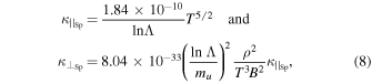
measured in SI units with ln Λ = 30.
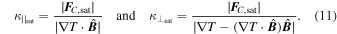
To limit the steep temperature gradients for the impulsive reconnection phase, the saturated heat flux is introduced as Balbus (1986),

where cs
is the sound speed and  . Balbus & McKee (1982) suggested using ϕ = 0.3. Then the saturation effects are included by the modified coefficients in Equation (7),

where
To complete the equations, the divergence-free condition (∇ · B = 0) is satisfied at all times of the evolution.
The background magnetic field is driven by a quadrupole source buried under the photosphere (y = 0) at the depth y = −d formalized by Forbes et al. (1994), and the preexisting flux rope carrying the cool prominence material is located at an adjusted height h0 on the verge of nonequilibrium to have an immediate eruption (Mei et al. 2012). In order to approximately hold the line-tied boundary condition at y = 0, we adopt a gravitationally stratified atmosphere with two thin layers of high density below the corona with the depths hpho and hchr. For simplicity, the coronal temperature is isothermal, given by Tcor = 106 K, while the temperature at the photosphere is set to Tpho = 4300 K for y ≤ hpho. And we eventually treat the chromospheric temperature (hpho ≤ y ≤ hpho + hcor) by a sine interpolation. The original flux rope has a radius of r and carries a constant current density jz inside. Following the work of Forbes (1990), we introduce a weak current density of a cosine shape distributed around the flux rope to smooth the sharp edge linked to the current density inside the flux rope. To achieve the force-free condition within the flux rope, we also add a guide field Bz , which takes the maximum at the center of the flux rope but vanishes at the edge of the rope. In addition, the flux rope includes the cool prominence material with a temperature of Tf = 5 × 10⁴ K, and the temperature in the thin shell around the flux rope is treated by a linear interpolation. The radiative cooling can be strong in the low-temperature and dense region at the center of the flux rope. The same setup of jz , Bz , and Tf can refer to Ye et al. (2019).
Given a characteristic length by L = 108 m, we set d = 0.4L, h0 = 0.61d, r = 0.125d, and hpho = hchr = 0.01L. The associated mass density distribution is derived according to hydrostatic equilibrium with a given number density n0 = 5 × 10¹⁶ m−3 at y = hpho + hcor, and the current density inside the flux rope is given by jz = 1.169 × 10⁻² A m−2. This yields a magnetic field of about 144 G at the origin. The resistivity is set to be uniform in the simulation domain at η = 5 × 10⁸ m2 s−1 to facilitate fast magnetic reconnection, which corresponds to a Lundquist number S = vA h0/η ≈ 105, with vA the Alfvén speed under the flux rope. The dynamic viscosity coefficient is set to be ν = 1 × 10⁸ kg m−1 s−1. Lastly, the line-tied condition is specified for the lower boundary, while open boundary conditions are utilized for the other boundaries, as implemented by Ye et al. (2019).
The 2.5D MHD simulation is performed by the MPI-parallelized AMR code NIRVANA3.8 (Ziegler 2004, 2005, 2008). The hyperbolic MHD system is solved by the second-order Godunov scheme, and the shock structures are accurately captured by the Harten–Lax–van Leer discontinuities Riemann solver (Miyoshi & Kusano 2005). The parabolic thermal conduction part is solved by the Super-TimeStepping method (Meyer et al. 2012). The divergence-free condition of the magnetic field (∇ · B = 0) is guaranteed by the constrained transport method. Since the initial magnetic field is obtained from the magnetic potential by B = ∇ × A , the vector B is accurately divergence-free. At last, all conserved parameters are updated explicitly in time by the third-order Runge–Kutta scheme.
Our simulation domain is defined by (x, y) ∈ [ − 3L, 3L] × [0, 8L], and a root grid of 600 × 800 is used. To handle the large density gradient close to the bottom, we also implement a static refinement (SMR) of a maximum four levels in this region. Four successive layers of SMR are settled before the computation starts: level 1 for y ≤ 0.04L, level 2 for y ≤ 0.03L, level 3 for y ≤ 0.02L, and level 4 for y ≤ 0.01L. Four levels of AMR are executed in the region −0.2L ≤ x ≤ 0.2L, and the finest cell size is 62.5 km. To quantitatively predict the contribution to heating the CME by turbulence, the conduction time, τc , and the radiation time, τr , are given in cgs units by

Yamamoto et al. (2002) suggested a temperature T ∼ 2 × 10⁶ K, number density ne
∼ 2 × 108 cm−3, and loop length Lc
∼ 2 × 1010 cm for a typical arcade system in the quiet region from the Yohkoh soft X-ray telescope data, the radiative cooling function Q(T) = 3.53 × 10⁻¹³
T−3/2 erg cm−3 s−1 for  (Klimchuk et al. 2008), and
  erg cm−1 s−1 K−1 from Equation (8). Then, we have τc
∼ 9.55 × 10³ and τr
∼ 3.32 × 10⁴ s. As the temperature increases due to reconnection heating, τc
will become much shorter than τr
. For the model used in our simulation, the CS exhaust cannot reach the prominence material in the original flux rope with the enclosed magnetic field inside (Lin et al. 2004). The heating of the prominence should be related to an intrinsic property of the moving flux rope other than turbulence in the CS. These facts reveal that thermal conduction is more important for this reconnection problem taking the turbulence into account, so the radiative cooling and the coronal heating functions are not included for simplicity.
erg cm−1 s−1 K−1 from Equation (8). Then, we have τc
∼ 9.55 × 10³ and τr
∼ 3.32 × 10⁴ s. As the temperature increases due to reconnection heating, τc
will become much shorter than τr
. For the model used in our simulation, the CS exhaust cannot reach the prominence material in the original flux rope with the enclosed magnetic field inside (Lin et al. 2004). The heating of the prominence should be related to an intrinsic property of the moving flux rope other than turbulence in the CS. These facts reveal that thermal conduction is more important for this reconnection problem taking the turbulence into account, so the radiative cooling and the coronal heating functions are not included for simplicity.
3. Simulation Results
Figure 1(a) shows the initial magnetic field and current density distribution. There is no CS at the beginning of the simulation. In Figure 1(b), we plot the temperature distribution around the flux rope, and the cool prominence material is colocated with the maximum current density at the center of the flux rope. The total force is defined as the sum of the pressure gradient, Lorentz force, and gravity force: F = − ∇p + J × B + ρ g . We calculated the total force field F upon the flux rope and found that the flanks of the flux rope are compressed. This force imbalance might be responsible for heating the prominence to the coronal temperature in the early stage of acceleration in this model. As mentioned earlier, the initial nonequilibrium state of the flux rope can lead to an immediate catastrophic evolution, and the CS is formed behind the rising flux rope. Figure 2 presents the time evolution of the mass density and temperature along the line x = 0 from t = 0 to 4205.3 s using level 4 of AMR. In panel (a), the discontinuities in the y-direction indicate the fast shock, the leading edge of the flux rope, and the center of the flux rope possessing the maximum density in the corona. The flux rope accelerates quickly in the early phase and subsequently rises at a nearly constant speed, while the CS thins and stretches following the evolution of the flux rope. As seen in panel (b), the original flux rope swells as it rises, which results in an increase of the density and temperature at the border. The saturation effect and numerical diffusion can lead to an effective perpendicular thermal conduction, as the temperature gradient becomes large in the flux rope. Then, the dense and hot source spreads into the prominence material, which is strongly heated to ∼106 K for the time t < 100 s and has a final temperature of ∼107 K. Note that this high final temperature of the prominence core is overestimated without radiative cooling in this model. Copious hot and dense plasmoids are generated and ejected bidirectionally in the CS starting from t = 617.4 s. Oscillation regions form at the upper and lower tips of the CS behind the TSs (Takasao & Shibata 2016; Takahashi et al. 2017). The upper oscillation region is known as the buffer region. The buffer region is compressed and heated by TSs, and upward-moving plasmoids can further heat this region when they collide.

Figure 1. (a) Initial magnetic configuration and current density distribution. (b) Temperature distribution and force balance of the flux rope (black arrows).
Download figure:
Standard image High-resolution image
Figure 2. Time–distance diagram of (a) mass density and (b) temperature on a log scale along the line x = 0.
Download figure:
Standard image High-resolution imageWe extract the global distributions at t = 1030.7 s and obtain the associated synthetic extreme-ultraviolet (EUV) images using the CHIANTI database (Dere et al. 1997), as shown in Figure 3. In panels (a)–(d), we plot the synthetic views in SDO/AIA 94, 131, 171, and 193 Å on logarithmic scale values of the radiation intensities denoted by lg(I). The bright CS, plasmoids, and hot exterior boundary of the CME bubble are easily identified in the AIA 94 and 131 Å channels. Also, complicated structures of the CME bubble are found in all four passbands. In panel (e), the heat originating from joule heating and slow-mode shocks inside the CS is mainly conducted along the magnetic field to arrive on the top of the CME bubble, and the thermal structure of the erupting bubble is generally in agreement with the observations of Cheng et al. (2018). Then, in panel (f), the density distribution presents the shell-like structures formed around the original flux rope, because the CME bubble is full of slow shocks within. The symbol "SS" is the abbreviation for "slow shocks," and the arrows indicate the location of the slow shocks. The Petschek-type slow-mode shocks generated from the principal X-point in the upflow region are confirmed by Mei et al. (2012), and they propagate to either side of the flux rope along the field lines identified from Rankine–Hugoniot relations (Shiota et al. 2005). Since the field above the flux rope is closed, slow shocks collide with each other on the top of the CME bubble, where the plasma density is weakly enhanced. The CME bubble expands continuously as it rises; thus, the inner boundary of the expanding bubble corresponds to the structure of slow shocks propagating from the base of the CME. In addition, the slow shocks continue to dissipate energy, heating the plasma inside the bubble. This might provide a reasonable explanation for the complicated structures of CMEs found in observations (Cremades & Bothmer 2004). Lastly, we show the 1D results of the former panels along the line x = 0 in the range 0.2L < y < 0.5L to study the properties of the TS under the flux rope in panel (g). The dashed line in this panel indicates the TS. As we can see, the jumps at the TS can be easily identified in all mentioned AIA wavelengths with the finest cell size (=62.5 km) in our simulation, and it is most significant in AIA 131 Å. However, when degraded into the AIA resolution (=435 km), the jumps of the TS under the flux rope are hardly detectable in all AIA wavelengths. The temperature of the CS generally decreases with height, and the temperature range is relatively narrow, which is consistent with Warren et al. (2018). For comparison, the jump in temperature of the TS seems smoother than that in density and is located slightly lower than the shock front, because the plasma in the upstream of the TS is preheated by thermal conduction (Takasao & Shibata 2016). It is worth noting that the compression ratio of the TS reaches nearly 4.27 here, which is beyond the ideal (adiabatic) limit of 4 for a shock. A compression ratio above 4 could be due to thermal conduction carrying energy away from the postshock gas, which allows more plasma to accumulate above the TS to balance the energy loss. As described in Ye et al. (2019), due to the lack of an effective constraint by the magnetic field, the plasma at the buffer region is roughly isotropic.

Figure 3. Global evolution and synthetic EUV images in the x–y plane at t = 1030.7 s. (a) AIA 94 Å; (b) AIA 131 Å; (c) AIA 171 Å; (d) AIA 193 Å; (e) temperature lg(T); (f) mass density lg(ρ); (g) 1D results of the former panels along the line x = 0 in the range of 0.2L < y < 0.5L. The dashed line identifies the location of the TS under the flux rope. The black solid lines represent the 1D profiles extracted from panels (a)–(f), while the red solid lines show the associated profiles degraded to the AIA resolution.
Download figure:
Standard image High-resolution imageLooking into the turbulence in the buffer region, we calculated the magnetic energy density  within. Figure 4 shows the distribution of
  and the corresponding spectrum in a box with a size of 0.2L × 0.1L using the 2D Fourier transform technique at t = 337.4 and 1039.9 s. Here we define kx = 0, 2π/Lx
, 2 × 2π/Lx
, 3 × 2π/Lx
, etc. and ky = 0, 2π/Ly
, 2 × 2π/Ly
, 3 × 2π/Ly
, etc., with Lx
= 0.2L and Ly
= 0.1L the length scales selected in the x- and y-directions. Also, the imaginary parts of the spectra with negative coordinates are drawn to better show the 2D Fourier spectra. At the early phase of the eruption at t = 337.4 s, a Y-structure is formed at the bottom of the CME, and the distribution of the power spectrum is peaked mainly at small kx, ky, which reveals that no small structures have appeared. Then, at a later time t = 1039.9 s, the buffer region becomes quite messy and the spectrum spreads out to larger kx, ky, indicating the local turbulent property with the generation of smaller-scale structures. Despite the big difference between 2D and 3D turbulence in the simulations, the fundamental physics in 2D, such as the energy conversion, reconnection rate, or particle acceleration, is still valid in 3D (Guo et al. 2014, 2015, 2016).
and the corresponding spectrum in a box with a size of 0.2L × 0.1L using the 2D Fourier transform technique at t = 337.4 and 1039.9 s. Here we define kx = 0, 2π/Lx
, 2 × 2π/Lx
, 3 × 2π/Lx
, etc. and ky = 0, 2π/Ly
, 2 × 2π/Ly
, 3 × 2π/Ly
, etc., with Lx
= 0.2L and Ly
= 0.1L the length scales selected in the x- and y-directions. Also, the imaginary parts of the spectra with negative coordinates are drawn to better show the 2D Fourier spectra. At the early phase of the eruption at t = 337.4 s, a Y-structure is formed at the bottom of the CME, and the distribution of the power spectrum is peaked mainly at small kx, ky, which reveals that no small structures have appeared. Then, at a later time t = 1039.9 s, the buffer region becomes quite messy and the spectrum spreads out to larger kx, ky, indicating the local turbulent property with the generation of smaller-scale structures. Despite the big difference between 2D and 3D turbulence in the simulations, the fundamental physics in 2D, such as the energy conversion, reconnection rate, or particle acceleration, is still valid in 3D (Guo et al. 2014, 2015, 2016).
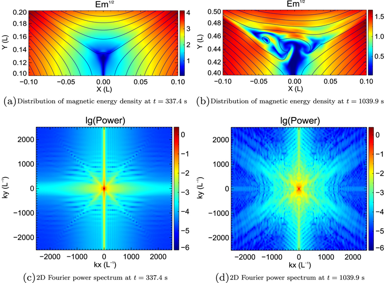
Figure 4. Distribution of magnetic energy density Em and the corresponding Fourier power spectrum in a box with a size of 0.2L × 0.1L covering the buffer region.
Download figure:
Standard image High-resolution imageThe turbulent energy is a fundamental parameter for studying the amplification of the magnetic field and particle acceleration, as the energy cascades into small scales. We show the turbulent properties of the TSs at the bottom of the CME before (t = 1030.7 s) and after (t = 1067.4 s) a plasmoid collision in Figure 5 from the outputs using level 4 of AMR. In panel (a), the velocity fields, fast magnetosonic Mach number (≥1), and plasma β are presented. Note that the Mach number is defined as  , where vflow, cs
, and vA are the local velocity, sound speed, and Alfvén speed, respectively. One can find a sharp drop in the velocity across the TSs for both times, while the plasma β sometimes shows no discontinuity at the TSs. The Mach number before the TS is 2.2–2.5 at t = 1030.7 s and becomes smoothly distributed with a value of 2.0–2.1 at t = 1067.4 s. In panel (b), the histograms of the upstream and downstream velocities of the TSs located in boxes 1 and 2 in the left column of panel (a) are shown. Here box 1 is chosen to be a small square completely included in the outflow region close to the shock front, and box 2 is the square with the same size behind the shock. At t = 1030.7 s, the geometry of TSs consists of two oblique shocks with a short horizontal shock in between. The average velocity in box 1 is computed to be about vu
= 650.2 km s−1 with a standard deviation of σu
= 14.9 km s−1, while that in box 2 is about vd
= 299.1 km s−1 with a standard deviation of σd
= 77.6 km s−1. The velocity variations provide an important quantity for the turbulent energy. The change of the standard deviation at t = 1030.7 s implies that the turbulence can be amplified by the TS by a factor of ∼5. Then, at t = 1067.4 s, the TS becomes generally horizontal. The average velocity in box 1 is vu
= 559.7 km s−1 with a standard deviation of σu
= 2.6 km s−1, while that in box 2 is vd
= 308.6 km s−1 with a standard deviation of σd
= 4.7 km s−1. At this time, the turbulence becomes weaker and is not amplified much by the TS. We stress that the size of the sampling box does not significantly change the standard deviation, as long as all data are selected in the outflow region close enough to the shock front. The different properties of the TSs at two times might be related to the local β ahead and behind. As seen in the right column of panel (a), the high β in the CS flows into the buffer region to make it more turbulent at t = 1030.7 s, while it does not do so at t = 1067.4 s. We have computed the standard deviation of the Mach number in box 1 denoted in panel (a) and obtained a value of 0.17 for t = 1030.7 s and 0.02 for t = 1067.4 s. Interestingly, the magnitude of the turbulence preshock might be related to the distribution of the Mach number of the TS. Since the Mach number can reveal the compression ratio of the shock, the bigger the Mach number is, the larger the enhancement factor of the postshock turbulent energy becomes. In order to compare the fraction of energy in turbulence with those in thermal and bulk kinetic energy, we compute the energy per unit mass. The ratio of the turbulent kinetic energy to the thermal energy of the shocked gas at t = 1030.7 s is
, where vflow, cs
, and vA are the local velocity, sound speed, and Alfvén speed, respectively. One can find a sharp drop in the velocity across the TSs for both times, while the plasma β sometimes shows no discontinuity at the TSs. The Mach number before the TS is 2.2–2.5 at t = 1030.7 s and becomes smoothly distributed with a value of 2.0–2.1 at t = 1067.4 s. In panel (b), the histograms of the upstream and downstream velocities of the TSs located in boxes 1 and 2 in the left column of panel (a) are shown. Here box 1 is chosen to be a small square completely included in the outflow region close to the shock front, and box 2 is the square with the same size behind the shock. At t = 1030.7 s, the geometry of TSs consists of two oblique shocks with a short horizontal shock in between. The average velocity in box 1 is computed to be about vu
= 650.2 km s−1 with a standard deviation of σu
= 14.9 km s−1, while that in box 2 is about vd
= 299.1 km s−1 with a standard deviation of σd
= 77.6 km s−1. The velocity variations provide an important quantity for the turbulent energy. The change of the standard deviation at t = 1030.7 s implies that the turbulence can be amplified by the TS by a factor of ∼5. Then, at t = 1067.4 s, the TS becomes generally horizontal. The average velocity in box 1 is vu
= 559.7 km s−1 with a standard deviation of σu
= 2.6 km s−1, while that in box 2 is vd
= 308.6 km s−1 with a standard deviation of σd
= 4.7 km s−1. At this time, the turbulence becomes weaker and is not amplified much by the TS. We stress that the size of the sampling box does not significantly change the standard deviation, as long as all data are selected in the outflow region close enough to the shock front. The different properties of the TSs at two times might be related to the local β ahead and behind. As seen in the right column of panel (a), the high β in the CS flows into the buffer region to make it more turbulent at t = 1030.7 s, while it does not do so at t = 1067.4 s. We have computed the standard deviation of the Mach number in box 1 denoted in panel (a) and obtained a value of 0.17 for t = 1030.7 s and 0.02 for t = 1067.4 s. Interestingly, the magnitude of the turbulence preshock might be related to the distribution of the Mach number of the TS. Since the Mach number can reveal the compression ratio of the shock, the bigger the Mach number is, the larger the enhancement factor of the postshock turbulent energy becomes. In order to compare the fraction of energy in turbulence with those in thermal and bulk kinetic energy, we compute the energy per unit mass. The ratio of the turbulent kinetic energy to the thermal energy of the shocked gas at t = 1030.7 s is  , since the magnetic energy before and behind the shock is small. Thus, the kinetic energy before the TS can be transferred into the thermal energy and turbulent kinetic energy through the shock. However, the small fraction of the energy that goes into turbulence indicates that, at least for our model parameters, the postshock turbulence does not have enough energy to account for the acceleration of nonthermal particles.

Figure 5. (a) Velocity field (left), Mach number (middle), and plasma β (right) at the bottom of the CME in (x, y) ∈ [−0.05L, 0.05L] × [0.4L, 0.5L] at t = 1030.7 and 1067.4 s. (b) Histograms of the velocity field in boxes 1 and 2 at t = 1030.7 s (first row) and t = 1067.4 s (second row). The white boxes in the left column of panel (a) are used to display the velocity variations upstream (marked by "1") and downstream (marked by "2") of the TSs.
Download figure:
Standard image High-resolution imageOn the other hand, the turbulence at the base of the CME is constantly sustained by the reconnection upflows, and the CME heating by turbulence could be important. In order to estimate it, we identified the location of the TS in the buffer region along the line x = 0 denoted by y = hTS(t). Then, we calculated the heating rate γheat and kinetic energy transfer rate γkinetic in the moving volume of Ω = [−0.06L, 0.06L] × [hTS − 0.02L, hTS + 0.1L] covering a small part of the upper CS, the TS, and the buffer region during the evolution. For a time step Δt, the rates are defined by

where m is the total mass of the volume Ω at time t, ETL and EKL are the thermal and kinetic energies confined in Ω at time t, ETI and EKI are the thermal and kinetic energies confined in Ω at time t − Δt, and ETF and EKF are the thermal and kinetic energies flowing into this region for Δt, respectively. The detailed calculation of the above variables is similar to that of Ni et al. (2012). Figure 6 shows the temporal energy transfer rates γheat and γkinetic from the formation of the CS at t = 122.4 s to the late time at t = 2699.7 s, taking a typical Δt ≈ 9.2 s. The heating rate increases greatly after the turbulence develops for t > 600 s. The violent variations in both rates reveal the intermittent energy releasing near the base of the CME. By integrating them on time, we obtain a cumulative heating rate of ∼4.09 × 10¹⁶ erg g−1 and a cumulative kinetic energy rate of ∼1.01 × 10¹⁶ erg g−1. Therefore, the plasma heating could be greater than the kinetic energy rate at the base of the CME. The cumulative heating rate here is of the same order as the fast blob E observed by the Ultraviolet Coronagraph Spectrometer (UVCS) during a CME on 2000 June 28 in the work of Murphy et al. (2011), indicating the significant plasma heating. From our calculation, the tearing CS, the TS, and the turbulence in the buffer region can make a nonnegligible contribution to the CME heating.

Figure 6. Energy transfer rates as a function of time from t = 122.4 to 2699.7 s in a volume around the buffer region. (a) Heating rate γheat. (b) Kinetic energy transfer rate γkinetic.
Download figure:
Standard image High-resolution imageWe also observe a set of waves near the base of the CME, as shown in Figure 7. The corresponding animation shows the generation of the wave trains continuously triggered by turbulence under the CME from t = 635.0 to 1308.3 s. In panel (a), the oblique TSs are well formed in the upflow region at t = 1039.9 s just before the plasmoid collision. In panel (b), the horizontal TS is formed between two oblique TSs under the CME at t = 1067.4 s after the plasmoid collision. In particular, some wavelike structures are identified outside the CS as coronal wave trains. Panel (c) presents the density distribution zoomed in on a smaller region and the velocity field within at t = 1039.9 s. One can find that the bottom of the CME is highly compressed by the reconnection outflow to form a downward magnetic tuning fork (MTF). The backflows inside propagate outward and compress the arms of the MTF again, similar to Takasao & Shibata (2016). Lastly, in panel (d), a plasmoid finished interacting with the MTF to make this region oscillate and become more turbulent. After the plasmoid collision at t = 1067.4 s, the arms of the MTF become flattened, and the oscillation is stabilized. Since the copious plasmoids are generated from the reconnection X-point, the continuous reconnection outflows and plasmoid collisions can maintain the oscillation. In this process, plenty of the propagating-outward fast-mode waves at higher altitudes originate from the turbulence. It is worth noting that, by comparing panels (a) and (b), only very faint waves can be seen near the base of the CME before a collision at t = 1039.9 s. This indicates that reconnection outflows can help the turbulence to develop and generate wave trains to propagate outward, but they are much weaker than those triggered by turbulence (or plasmoids).
Figure 7. (a) Divergence of velocity at t = 1039.9 s. (b) Divergence of velocity at t = 1067.4 s. (c) Mass density distribution in a smaller region at t = 1039.9 s. (d) Mass density distribution in a smaller region at t = 1067.4 s. The solid lines denote magnetic lines. The vertical dashed line in panel (b) indicates the location x = −0.15L, and the arrows in panels (c) and (d) represent the velocity fields. The animation presents the evolution of the divergence of velocity shown in panels (a) and (b) for a short period of time to display the continuous generation of wave trains.
(An animation of this figure is available.)
Download figure:
Video Standard image High-resolution imageIn order to study the dynamical behavior of the wave trains outside the CS, we plot the time–distance diagram of the normalized running difference of the density Δρ/ρ along the line x = −0.15L from t = 857.9 to 2038.6 s in Figure 8(a). There are violent variations below the edge of the CME, and they may have quasiperiodic behavior indicating the propagation of the coronal wave trains. Since the flux rope keeps rising, it is impossible to fix a point aside to check the periodicity of the wave trains. The estimation of the periodicity is also sensitive to the chosen line, along which the calculation is executed. For instance, we followed the dashed line almost parallel to the edge of the CME from panel (a). The associated distribution shows periodicity in panel (b), and the period is calculated to be ∼76.3 s. Therefore, we directly investigate the evolution of the turbulent region above the upper TS.

Figure 8. (a) Normalized running difference of the density along the line x = −0.15L extracted from t = 857.9 to 2038.6 s. The blue diagonal line corresponds to the low-density wing to the left of the TS in Figure 2(f), and the red diagonal line is where the density jumps back to the coronal value outside the flux rope. (b) Associated distribution along the dashed line in panel (a). The symbol Δρ/ρ is defined as (ρ(t) − ρ(t − Δt))/ρ(t). A typical Δt ≈ 9.2 s.
Download figure:
Standard image High-resolution imageTakasao & Shibata (2016) described how the CS outflow can form a blob of gas between the sides of a "tuning fork" and how the backflow of the gas drives an oscillation of the magnetic structure. The oscillation can drive waves that propagate well outside the "buffer region" where it occurs. Figures 7(c) and (d) show the dynamics of the backflow. The relation between the coronal wave trains and the turbulence under the CME is analyzed in Figure 9. In panel (a), we show the time evolution of the maximum of the horizontal velocity Vx of the backflow and the fast magnetosonic Mach number before the upper TS. Note that the Mach number is defined as the ratio of the flow velocity to the fast-mode magnetosonic speed. The max(Vx ) decreases in general, indicating that the coronal wave trains may appear at different speeds, which could be caused by variations in the local plasma density and magnetic strength. The peaks reveal the oscillation of the MTF. Interestingly, one can find that the Mach number mainly varies around 2.4, which is larger than that before the TS above the flare loops (1.5–1.8 found in observations and simulations; Chen et al. 2015; Ye et al. 2019). This reveals that it is easier to form the upper TS than the lower one, and the variation of the Mach number is related to the interplay between plasmoids and the TS (Shen et al. 2018). Then, we performed the Morlet transform on max(Vx ) to obtain the wavelet spectrum in panel (b), where the black solid line indicates the 95% significance level. Accordingly, the propagation of the coronal wave trains shows periodicity, and the corresponding period is computed to be 148.8 ± 30 s. Using the same method, we obtained a very similar result for the period of the Mach number. These periods are found to be much larger than that in Figure 8(b). Therefore, a set of strong subwaves are generated by turbulence instead of the primary reconnection outflows in the wake of the CME.

Figure 9. Relation between the coronal wave trains and the turbulence in the buffer region. (a) Maximum of the horizontal velocity Vx of the backflow (black) and the magnetosonic Mach number before the upper TS (red) from t = 857.9 to 2592.0 s. (b) Wavelet spectrum of the horizontal velocity of the backflow.
Download figure:
Standard image High-resolution image
4. Conclusion and Discussion
The CME plasma is strongly heated far from the flare arcade during the eruption, but the heating mechanism is not understood. The upflow from the CS, small-scale reconnection, and slow shocks are competing candidate mechanisms responsible for heating the ejected plasma (Lin et al. 2004; Shiota et al. 2005). Heating rates have been determined for several CMEs (Akmal et al. 2001; Lee et al. 2009; Landi et al. 2010; Murphy et al. 2011), and the heat deposited is comparable to the kinetic energy of the CME core. From our simulation, the heat from Joule heating and slow shocks is mainly conducted along magnetic fields to form the hot exterior boundary of the CME. The complicated internal structures of the CME in EUV images are related to the structure of slow shocks. In particular, the energy release via TSs and plasmoid collisions under the CME is substantial, and the heating rate is found to be greater than the kinetic energy transfer rate by taking into account the effect of turbulence. The buffer region under the CME is highly compressed by the TSs, and the compression ratio can exceed 4. But such a strong TS still cannot be easily detected in the AIA passbands because of the limited spatial resolution. Interestingly, the turbulence can be somewhat amplified by the TS under the CME, and the enhancement factor might be related to the local Mach number of the TSs. The ratio of the turbulent energy of the shocked gas to the thermal energy is quite small. Since only a few percent of the energy dissipated at the CME shock takes the form of postshock turbulence, and the rest goes into kinetic or thermal energy of the hot gas, there might not be enough turbulent energy to make a major contribution to particle acceleration in our simulation. However, it is plausible that oscillations in the post-TS regions could release energy to produce intermittency in HXRs and other quasiperiodic phenomena.
The mechanism for the prominence heating is still an open question. By considering the current density, resistivity, and mass in the initial flux rope from our simulation, we derive an expected heating rate of ∼1.9 × 10¹⁵ erg g−1 for the same propagation time of Figure 6. It seems that this estimate is over 1 order of magnitude smaller than the cumulative heating rate (∼4.09 × 10¹⁶ erg g−1) from the turbulent buffer region and cannot support the strong internal heating of the prominence. Thermal conduction from the hot gas into the core is prohibited by the magnetic field geometry in our 2.5D simulation but may occur in a complex 3D case. The 3D simulations will be performed to specifically study the intrinsic property of the prominence in the future.
Coronal wave trains at higher altitudes under the CME were noticed. It seems that the buffer region repeatedly forms a downward MTF, and outward-propagating backflows are excited by reconnection outflows and plasmoids to generate fast waves. The reconnection outflows can generate weak wave trains, while the plasmoids can generate much stronger ones. By studying the quasiperiodic features of the maximum horizontal velocity of the backflows, as well as the Mach number before the TS, we found that they both show periodicity, and their periods are very close to each other. It implies that the turbulence is an important contributor to the generation of the coronal wave trains around the CME.
The hot, dense region just above the upper TS in our simulation has not yet been reported in AIA observations of solar eruptions. However, it may have been detected in UVCS observations of fast CMEs from X-class flares. In those observations, the UVCS entrance slit was held at a constant height as the CME crossed it. In several cases, [Fe xviii] emission ( ) was observed for a few minutes just after the CME disrupted the preflare streamer; then it vanished (Raymond et al. 2003). The 2002 April 21 event in particular showed [Fe xviii] from a small region apparently near the base of the flux rope.
The authors would like to thank the anonymous referee for the valuable comments and suggestions that improved this work significantly. This work was supported by the Strategic Priority Research Program of CAS with grant XDA17040507, National Natural Science Foundation of China (NSFC) grants 12073073 and 11933009, and grants associated with the Yunling Scholar Project of the Yunnan Province and the Yunnan Province Scientist Workshop of Jun Lin. The calculations were carried out at the National Supercomputer Center in Tianjin on the Tianhe 1A, and the image processing was performed on the cluster in the Computational Solar Physics Laboratory of Yunnan Observatories. C.Q. was supported by the Natural Science Foundation of Henan Province 212300410210. M.Z. acknowledges the support by the NSFC grant U2031141 and the Applied Basic Research of Yunnan Province 2019FB005.
Software: NIRVANA 3.8.