


Abstract
We present results of subarcsec Atacama Large Millimeter/submillimeter Array observations of CO(2–1) and CO(5–4) toward a massive main-sequence galaxy at z = 1.45 in the Subaru-XMM/Newton Deep Survey/UDS field, aiming at examining the internal distribution and properties of molecular gas in the galaxy. Our target galaxy consists of the bulge and disk, and has a UV clump in the Hubble Space Telescope images. The CO emission lines are clearly detected, and the CO(5–4)/CO(2–1) flux ratio (R52) is ∼1, similar to that of the Milky Way. Assuming a metallicity-dependent CO-to-H2 conversion factor and a CO(2–1)/CO(1–0) flux ratio of 2 (the Milky Way value), the molecular gas mass and the gas-mass fraction (fgas = ratio of the molecular gas mass to the molecular gas mass + stellar mass) are estimated to be ∼1.5 × 10¹¹M⊙ and ∼0.55, respectively. We find that R52 peak coincides with the position of the UV clump and that its value is approximately twice higher than the galactic average. This result implies a high gas density and/or high temperature in the UV clump, which qualitatively agrees with a numerical simulation of a clumpy galaxy. The CO(2–1) distribution is well represented by a rotating-disk model, and its half-light radius is ∼2.3 kpc. Compared to the stellar distribution, the molecular gas is more concentrated in the central region of the galaxy. We also find that fgas decreases from ∼0.6 at the galactic center to ∼0.2 at three times the half-light radius, indicating that the molecular gas is distributed in the more central region of the galaxy than stars and seems to be associated with the bulge rather than with the stellar disk.
Export citation and abstract BibTeX RIS
1. Introduction
Understanding when and how disk galaxies form is one of the very important subjects in modern astrophysics. The density of the cosmic star formation rate (SFR) increases from the early universe, peaks at z ∼ 1–3, and decreases by one order of magnitude to the present day (e.g., Madau & Dickinson 2014). Galaxies are thought to evolve drastically at z ∼ 1–3, and thus observing galaxies at this redshift range is indispensable for understanding galaxy formation and evolution.
Recent deep imagings with high angular resolution by the Hubble Space Telescope (HST) enable us to resolve the structure of galaxies at z ∼ 1–3 on subkiloparsec scale in the rest-frame UV to optical bands. A galaxy population resembling the present-day disk galaxies emerges from z ∼ 2 − 3 (e.g., Cameron et al. 2011; Mortlock et al. 2013; Talia et al. 2014), and at z ∼ 0.8, the fundamental structure of the disks seems to be already matured (e.g., Lilly et al. 1998; Takeuchi et al. 2015). Bulge-like structures are also seen in disk-like galaxies at z ∼ 1–2 in the rest-frame optical band (e.g., Cameron et al. 2011). These observational features suggest that the disk galaxies acquire their nature as seen in the local universe during the period around at z ∼ 1–3.
About half of the star-forming galaxies (SFGs) at this redshift range show clumpy structures in rest-frame UV band (e.g., Elmegreen et al. 2007; Guo et al. 2015; Shibuya et al. 2016). These "clumpy" galaxies are thought to evolve into the present-day disk galaxies. Observational studies reveal that the clumps have a stellar mass of ∼108−10 M☉, SFR of ∼1–100 M☉ yr−1, size of 1–2 kpc, and age of ∼107−9 yr. The clumps close to the center of the host galaxy show a higher stellar mass, redder color, and older age than the clumps that reside in the outer part (e.g., Förster Schreiber et al. 2011; Guo et al. 2012, 2018). This trend is explained by a theoretical scenario that a gas-rich disk forms through a cold gas that was accreted from a dark matter halo and/or streamed from the outside of the galaxy, and that clumps form through gravitational instability in the gas disk. Because of the dynamical friction and/or dynamical interaction, the clumps migrate toward the center of the disk and eventually coalesce into a young bulge (e.g., Noguchi 1999; Bournaud et al. 2014).
Meanwhile, the inside-out growth of galaxies is also one aspect of observational results. For massive SFGs (Mstar ≳ 1011 M☉), no significant increase of stellar mass is seen in the central region of galaxies since z ∼ 2, and most of new mass growth is seen in the outer region (e.g., van Dokkum et al. 2010; Patel et al. 2013; Tacchella et al. 2018). For less massive SFGs, the mass growth is seen at all galactic radii, suggesting a synchronous growth of the bulge and disk at z ≳ 1, while z ≲ 1 the stellar mass growth gradually halts in the central region, even though the mass growth continues in the outer region (e.g., van Dokkum et al. 2013; Tacchella et al. 2018). From an analysis of main-sequence galaxies with Mstar > 1010 M☉ at z ∼ 1–3, Margalef-Bentabol et al. (2018) showed that the bulge-to-disk SFR ratio decreases from z ∼ 3 to ∼1, which suggests inside-out quenching of star formation.
The properties of molecular gas in SFGs at z ∼ 1–3 have recently been investigated. The cosmic molecular gas density evolves similarly to the cosmic SFR density: it peaks at z ∼ 1–3 and is higher than the local value by approximately one order of magnitude (e.g., Maeda et al. 2017; Decarli et al. 2019; Riechers et al. 2019). Observations of molecular gas in main-sequence SFGs at this redshift range reveal that gas-mass fractions (fgas = Mgas/(Mgas + Mstar), where Mgas refers to a molecular gas mass) are higher (typically, fgas ∼ 0.5; e.g., Tacconi et al. 2013; Seko et al. 2016) than those of local galaxies (typically, fgas ≲ 0.1). The average CO excitation of SFGs (sBzK galaxies) at z ∼ 1.5 is significantly higher than that of the Milky Way (e.g., Carilli & Walter 2013; Daddi et al. 2015), suggesting that the physical conditions of the molecular gas are different. In order to understand galaxy evolution further, observations of the distribution of molecular gas in normal SFGs including clumpy galaxies on subkiloparsec scale are inevitable. However, resolving the distribution of the molecular gas in high-redshift galaxies is still challenging and is limited to some particular cases such as submillimeter galaxies and gravitationally lensed systems (for a review, see Hodge & da Cunha 2020). Our knowledge of the spatial distribution of molecular gas and its properties in SFGs at z ∼ 1–3 is still poor.
In this paper, we present results of subarcsecond Atacama Large Millimeter/submillimeter Array (ALMA) observations of CO(2–1) and CO(5–4) emission lines toward a massive main-sequence galaxy at z = 1.45 in the Subaru-XMM/Newton Deep Survey (SXDS; Furusawa et al. 2008) field. The CO observations toward this galaxy enable us to study molecular gas properties in a normal SFG with a UV clump around at the peak of the cosmic SFR density. Combining multitransition CO data and high-resolution HST data of the galaxy, we also study the CO(5–4)/CO(2–1) flux ratio in the UV clump. Through model fitting, we compare the properties of the molecular gas and stellar distributions, and we also reveal the radial profile of the gas-mass fraction.
This paper is structured as follows: in Section 2 we present the properties of our sample galaxy. The ALMA observations, the data reductions, and the archival HST data are described in Section 3. The results and discussions are provided in Section 4. We report molecular gas properties and distributions in Section 4.1 and stellar distributions in Section 4.2. In Section 4.3 we compare the molecular gas and stellar distributions. Finally, we present the summary in Section 5. Throughout this paper, we adopt a flat cosmology with ΩM
= 0.3, ΩΛ = 0.7 and H0 = 70 km s−1 Mpc−1. At the redshift of our sample galaxy (z = 1.450), the linear scale is  . The initial mass function (IMF) of Chabrier (2003) is adopted. Magnitudes are in the AB system unless otherwise noted.
2. Sample Galaxy
The sample galaxy in this study, SXDS1_13015, is one of the most massive main-sequence galaxies at z ∼ 1.4 in the sample galaxies by Yabe et al. (2012) and Seko et al. (2016). Using the Fiber Multi-Object Spectrograph on the Subaru telescope, Yabe et al. (2012) made near-infrared spectroscopic observations of 317 Ks-band-selected SFGs at z ∼ 1.4 in the SXDS/UDS (UKIRT Infrared Deep Sky Survey Ultra Deep Survey; Lawrence et al. 2007) field. The stellar masses were derived by fitting the spectral energy distribution (SED) with optical to mid-infrared data, adopting the stellar population synthesis model by Bruzual & Charlot (2003) and the IMF by Salpeter (1955). The SFRs were derived from extinction-corrected rest-frame UV luminosity densities by using the conversion factor by Kennicutt (1998), where the extinction law of Calzetti et al. (2000) was assumed and the color excesses were estimated from the rest-frame UV slopes. After we corrected for the difference of the adopted IMF with a factor of 0.58 (Speagle et al. 2014), the stellar mass and SFR of SXDS1_13015 are ∼1.2 × 10¹¹ M☉ and ∼130 M☉ yr−1, respectively. Hα emission lines were detected from 71 galaxies including SXDS1_13015, and the gas metallicities were derived based on the N2 method (Pettini & Pagel 2004).
Using ALMA, Seko et al. (2016) made observations of 12CO(5–4) and dust thermal emission toward 20 SFGs selected from the sample galaxies by Yabe et al. (2012). Twenty SFGs were selected to uniformly cover a wide range of stellar mass (4 × 10⁹ − 4 × 10¹¹
M☉) and metallicity ( ) in the diagrams of stellar mass versus SFR and the stellar mass versus metallicity. CO(5–4) lines are detected toward 11 galaxies, and dust emissions are clearly detected from 2 galaxies. Both CO emission and dust thermal emission were detected for SXDS1_13015. When a metallicity-dependent CO-to-H2 conversion factor (Genzel et al. 2012) and CO(5–4)/CO(1–0) luminosity ratio of 0.23 (typical for sBzK galaxies by Daddi et al. 2015) are adopted, the molecular gas mass of SXDS1_13015 is estimated to be ∼1 × 10¹¹
M☉. Using a modified blackbody model with a dust temperature of 30 K and a dust emissivity index of 1.5, the dust mass of SXDS1_13015 is estimated to be ∼5 × 10⁸
M☉.
) in the diagrams of stellar mass versus SFR and the stellar mass versus metallicity. CO(5–4) lines are detected toward 11 galaxies, and dust emissions are clearly detected from 2 galaxies. Both CO emission and dust thermal emission were detected for SXDS1_13015. When a metallicity-dependent CO-to-H2 conversion factor (Genzel et al. 2012) and CO(5–4)/CO(1–0) luminosity ratio of 0.23 (typical for sBzK galaxies by Daddi et al. 2015) are adopted, the molecular gas mass of SXDS1_13015 is estimated to be ∼1 × 10¹¹
M☉. Using a modified blackbody model with a dust temperature of 30 K and a dust emissivity index of 1.5, the dust mass of SXDS1_13015 is estimated to be ∼5 × 10⁸
M☉.
The properties of SXDS1_13015 are summarized in Table 1. Figure 1 (left) shows the composite image of HST WFC3 F160W (hereafter, H160), F125W (J125), and ACS F606W (V606). The galaxy seems to consist of the bulge and disk. In the disk, an arm-like feature is seen in particular at the northeastern side of the galaxy. Figure 1 (right) shows an HST V606 image corresponding to the rest-frame UV (∼2500 Å). The image clearly shows the presence of a UV clump located at ∼ 0 3 north of the center, which is also a UV bright region.
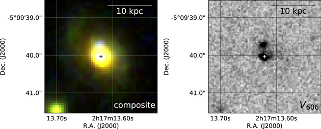
Figure 1. Left: composite image of HST WFC3/IR H160, J125, and ACS/WFC V606 (R, V, and U band in the rest-frame, respectively) images of SXDS1_13015. The cross shows the peak position of J125. Right: same as the left panel, but for the V606-band image. SXDS1_13015 has a UV clump at ∼03 north of the galactic center (cross).
Download figure:
Standard image High-resolution imageTable 1. Properties of SXDS1_13015
| R.A. (J2000) a | 02h17m13 62 62 |
| Decl. (J2000) a | −05°09'400 |
| zCO b | 1.4500 ± 0.0002 |
| Mstar (M☉) c , d |

|
| SFR (M☉ yr−1) d | 128 ± 32 |
 e
e
| 8.85 ± 0.04 |
| E(B − V) (mag) f | 0.49 |
Notes.
a Coordinate of the peak pixel of the CO(2–1) 0th moment map. b Redshift derived from the CO(2–1) line profile. c Derived from the SED fitting with optical to mid-infrared data. d A Chabrier IMF is adopted. The difference of the adopted IMF is corrected with a factor of 0.58 (Speagle et al. 2014). The SFR is derived from the extinction-corrected UV luminosity density. e Derived with the N2 method. A Pettini & Pagel (2004) calibration is adopted. f Derived from the rest-frame UV slope.Download table as: ASCIITypeset image
3. Data Sources
3.1. CO Data
Observations of 12CO(2–1) toward SXDS1_13015 were made with ALMA on 2016 August 24 and September 3 during ALMA Cycle3 (ID: 2015.1.01129.S, PI: K. Ohta). Forty-one 12 m antennas were used. The length of the longest and shortest baseline was 1.8 km and 15.1 m, respectively, corresponding to an angular resolution of ∼055 and a maximum recoverable scale of ∼11''. The observed frequency range was 93.598–94.535 GHz (band 3) to detect the 12CO(2–1) emission line (νrest = 230.538 GHz, νobs = 94.097 GHz) with a bandwidth of 937.5 MHz and a spectral resolution of 564.453 kHz, corresponding to a velocity range and resolution of 2988 km s−1 and 1.8 km s−1, respectively. The total on-source time was 4.7 hr. J0006-0623 and J0238-1636 were used as the flux, bandpass, and amplitude calibrators. The phase calibrators were J0209-0438 and J0215-0222.
The details of the CO(5–4) observations are described by Seko et al. (2016). The observation was conducted during ALMA Cycle 0 (ID: 2011.0.00648.S, PI: K. Ohta), and the angular resolution was ∼07. The observed frequency range was 222.094–252.583 GHz (band 6), the spectral resolution was 488.28 kHz (∼0.6 km s−1), and the on-source time was ∼10 minutes.
The raw visibility data of CO(2–1) were calibrated with the Common Astronomy Software Applications (CASA; McMullin et al. 2007) version 4.7.2 and the observatory-provided calibration script. The raw visibility data of CO(5–4) were calibrated with CASA version 4.2 by Seko et al. (2016). The imagings of the ALMA data were carried out using CASA version 5.4.0. In order to make cleaned channel maps of CO(2–1) and CO(5–4), we used the CASA tasks uvcontsub and tclean. First, the continuum emission in the CO(5–4) data was subtracted with the uvcontsub. After this, we made 3σ-clean channel maps of CO(2–1) and CO(5–4) using the tclean with a Briggs weighting (robust = 0.5) and a channel width of 25 km s−1. The synthesized beam sizes of the CO(2–1) and CO(5–4) channel maps were 061 × 052 (∼4.8 kpc) and 084 × 060 (∼6.0 kpc), respectively. The noise levels of CO(2–1) and CO(5–4) at the velocity width of 25 km s−1 were 0.18 mJy beam−1 and 0.91 mJy beam−1, respectively.
3.2. HST Data
SXDS1_13015 is located in the UKIDSS UDS field, and has been imaged with HST ACS, WFC3/UVIS, and WFC3/IR as part of the Cosmic Assembly Near-infrared Deep Extragalactic Legacy Survey (CANDELS; Grogin et al. 2011; Koekemoer et al. 2011) observations. We used the archival ACS V606, WFC3 J125, and H160 data on the CANDELS website.
4
The images are drizzled and the pixel scales are 003 for V606 and 006 for J125 and H160.
4. Results and Discussions
4.1. Molecular Gas Properties
The integrated CO(2–1) and CO(5–4) intensity maps (0th moment maps) and the line profiles of SXDS1_13015 are shown in Figure 2. The symmetric double-peak line profile of CO(2–1) implies that the galaxy has a rotating gas disk. The peak position of the CO(5–4) image shows a slight (∼015) offset from that of the CO(2–1) image, and an asymmetry is seen in the CO(5–4) line profile. These features originate from the presence of the UV clump, as described below (Section 4.1.2). Thus we adopt the peak in the CO(2–1) map as the center of the galaxy, and the central frequency of the observed CO(2–1) emission line (94.097 ± 0.008 GHz, corresponding to a redshift of 1.4500 ± 0.0002) is taken as the zero velocity.
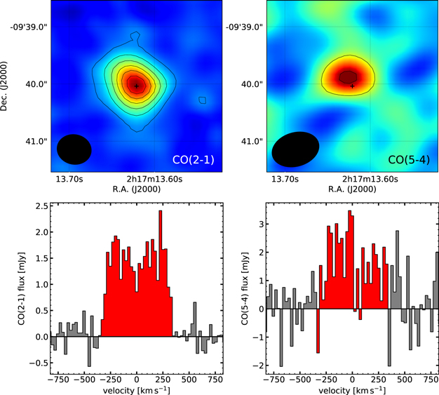
Figure 2. Top: integrated intensity maps (0th moment maps) of CO(2–1) (left) and CO(5–4) (right) integrated over the velocity range shown in red in the line profiles (bottom panels). The contours represent 3σ, 7σ, 11σ, etc. (4σ steps). The black crosses show the CO(2–1) peak position. The filled black ellipse in the bottom left corner shows the synthesized beam size. Bottom: line profiles of CO(2–1) (left) and CO(5–4) (right) in circles with 15 diameter. In the CO(2–1) profile, the emission line of SXDS1_13015 is shown in red. In the CO(5–4) profile, the same velocity range with the CO(2–1) profile is also shown in red.
Download figure:
Standard image High-resolution image4.1.1. Total Flux and Molecular Gas Mass
The total CO(2–1) and CO(5–4) fluxes of SXDS1_13015 are derived by fitting an elliptical Gaussian model to the respective integrated intensity maps. We use the data in a circle of 15 diameter centered on the peak of the CO(2–1) integrated intensity map. The total CO(2–1) and CO(5–4) fluxes of SXDS1_13015 are estimated to be (1.03 ± 0.05) Jy km s−1 and (1.16 ± 0.17) Jy km s−1, respectively. The beam-deconvolved full width at half maximum of the CO(2–1) source is 4.0 ± 0.5 kpc. The CO(5–4) flux value is different from that derived by Seko et al. (2016) because the adopted velocity width and the data reduction are different.
The CO(5–4)/CO(2–1) flux ratio (R52 = SCO(5–4)Δv/SCO(2–1)Δv) is 1.1 ± 0.2, which suggests that the CO excitation ladder of SXDS1_13015 is similar to that of the Milky Way rather than to color-selected SFGs at z ∼ 1–3 (Carilli & Walter 2013). 5 Low CO excitations like this are also reported in some SFGs at z ∼ 1–2.5 (e.g., Decarli et al. 2016).
We calculate the total CO(1–0) luminosity ( ) as
) as
where  is measured in K km s−1 pc2, νrest:CO(1–0) is the rest frequency of the CO(1–0) emission line of 115.271 GHz, DL
is the luminosity distance in Mpc, R21 is the CO(2–1)/CO(1–0) flux ratio, and SCO(2–1)Δv is the observed CO(2–1) flux in Jy km s−1. Because the CO excitation ladder of the galaxy is similar to that of the Milky Way, we assume R21 = 2. The calculated total CO(1–0) luminosity of SXDS1_13015 is (5.62 ± 0.27) × 1010 K km s−1 pc2.
is measured in K km s−1 pc2, νrest:CO(1–0) is the rest frequency of the CO(1–0) emission line of 115.271 GHz, DL
is the luminosity distance in Mpc, R21 is the CO(2–1)/CO(1–0) flux ratio, and SCO(2–1)Δv is the observed CO(2–1) flux in Jy km s−1. Because the CO excitation ladder of the galaxy is similar to that of the Milky Way, we assume R21 = 2. The calculated total CO(1–0) luminosity of SXDS1_13015 is (5.62 ± 0.27) × 1010 K km s−1 pc2.
The molecular gas mass is derived from

where αCO is the CO-to-H2 conversion factor in  . αCO in SFGs at z ∼ 1–2 is expected to depend on gas metallicity; the value of αCO is higher in galaxies with lower metallicity (Wolfire et al. 2010; Bolatto et al. 2013). As the dependence of αCO on metallicity, we adopt the Equation (7) of Genzel et al. (2015),

where αCO includes a 36% mass contribution of helium and  is the metallicity based on the Pettini & Pagel (2004) calibration. The αCO of SXDS1_13015 is calculated to be
  . The resulting total molecular gas mass is (1.45 ± 0.07) × 1011
M☉ and the gas-mass fraction is fgas = 0.55 ± 0.08. The gas-depletion time (τdepl = Mmol/SFR) of the galaxy is estimated to be = 1.1 ± 0.3 Gyr. The derived molecular gas properties of SXDS1_13015 are listed in Table 2.
. The resulting total molecular gas mass is (1.45 ± 0.07) × 1011
M☉ and the gas-mass fraction is fgas = 0.55 ± 0.08. The gas-depletion time (τdepl = Mmol/SFR) of the galaxy is estimated to be = 1.1 ± 0.3 Gyr. The derived molecular gas properties of SXDS1_13015 are listed in Table 2.
Table 2. Molecular Gas Properties of SXDS1_13015
| SCO(2–1)Δv (Jy km s−1) | 1.03 ± 0.05 |
| SCO(5–4)Δv (Jy km s−1) | 1.16 ± 0.17 |
| R52 a | 1.1 ± 0.2 |
 b
b
| (5.62 ± 0.27) × 1010 |
| Mmol (M☉) c | (1.45 ± 0.07) × 1011 |
| fgas d | 0.55 ± 0.08 |
| τdepl (Gyr) e | 1.1 ± 0.3 |
Notes.
a CO(5–4)/CO(2–1) flux ratio. b We adopt a CO(2–1)/CO(1–0) flux ratio of 2 (the Milky Way-like value). c Including a 36% mass contribution of helium. The metallicity-dependent CO-to-H2 conversion factor (Equation (7) of Genzel et al. 2015) is adopted. d Gas-mass fraction ( = Mmol/(Mmol + Mstar)). e Gas-depletion time ( = Mmol/SFR)Download table as: ASCIITypeset image
4.1.2. Spatial Distribution of R52
We made the R52 map by dividing the CO(5–4) 0th moment map by the CO(2–1) map convolved to the same beam size as the CO(5–4) data. R52 is calculated in pixels with a signal-to-noise ratio (S/N) > 2.5 in the CO(5–4) map. The resulting CO flux ratio map is shown in Figure 3. The peak of the CO(5–4)/CO(2–1) flux ratio (R52 ∼ 2.2) is significantly higher than the R52 averaged over SXDS1_13015 and that of the Milky Way. The ratio is comparable to the average R52 for sBzK galaxies at z ∼ 1.5 (Daddi et al. 2015). The peak of the flux ratio is located at ∼ 03 north of the peak of the CO(2–1) distribution (cross in Figure 3).

Figure 3. Spatial distribution of R52 in SXDS1_13015. The pixels with S/N > 2.5 in the CO(5–4) map are displayed. The contours represent 10%, 30%, etc. to 90% pixel values of the rest UV image relative to the peak of the galaxy. The black cross and ellipse show the CO(2–1) peak position and the synthesized beam size, respectively.
Download figure:
Standard image High-resolution imageInterestingly, the location coincides with the UV clump. The velocity at this position is ∼−150 km s−1 in the CO(2–1) velocity field (Figure 4), and this velocity corresponds to the peak velocity in the CO(5–4) profile (Figure 2, bottom right); the asymmetric feature of the CO(5–4) profile is presumably due to this component. We show the 0th moment maps integrated over the velocity range of −250 km s−1 to 0 km s−1 in Figure 5. The R52 map in this velocity range also peaks at the position of the UV clump. In the UV clump, it is expected that the density and/or temperature of the molecular gas are higher than those in other regions. This result, the high R52 in the UV clump, is qualitatively consistent with the CO excitation ladder modeled by a large velocity gradient analysis of the hydrodynamically simulated high-z clumpy galaxy (Bournaud et al. 2015).

Figure 4. Velocity field (1st moment map) of SXDS1_13015. The contours show the rest UV distribution (same as Figure 3). The black cross and solid line show the CO(2–1) peak position and the major axis of the galaxy, respectively. The filled black ellipse in the bottom left corner shows the synthesized beam size.
Download figure:
Standard image High-resolution image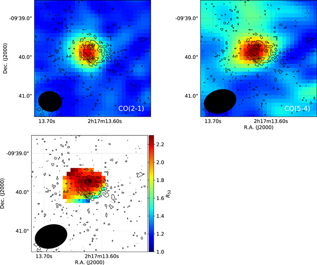
Figure 5. Top left: CO(2–1) 0th moment map integrated over the velocity range of −250 to 0 km s−1. The contours show the rest UV distribution (same as Figure 3). The black cross and the ellipse show the CO(2–1) peak position in the total integrated map and the synthesized beam size, respectively. Top right: same as the top left panel, but for CO(5–4). Bottom left: same as Figure 3, but for the velocity range of −250 to 0 km s−1.
Download figure:
Standard image High-resolution imageIt is worth noting that the spatial offset and the asymmetric profile of CO(5–4) are not results of noise. We performed simulations of the CO(5–4) observation with the CASA task simobserve assuming a Gaussian distribution, mimicking the CO(5–4) distribution and line profile. Consequently, we found that the 1σ uncertainty of the peak position of CO(5–4) is ∼004. The observed offset between the peak positions of CO(5–4) and CO(2–1) is ∼015, which corresponds to ∼3.8σ. We also found that the 1σ uncertainty of the peak velocity is ∼30 km s−1. The observed peak CO(5–4) velocity and the central CO(2–1) velocity is ∼ 150 km s−1, which corresponds to ∼5σ. Thus the offset and the peak velocity difference are considered to be real. It should also be noted here that we made astrometric corrections to the HST images with the offset shown below. We assume that the peak of J125 image coincides with the peak of the CO(2–1) 0th moment map because the CO(2–1) shows a good symmetry in the line profile and the S/N of the image is high. The offset is (ΔR. A.,Δdecl. ) = (+0058, −0198). Similar amounts of the offset between ALMA astrometry and HST astrometry are also reported in the Hubble Ultra-Deep Field and CANDELS GOODS-S region (Barro et al. 2016; Rujopakarn et al. 2016; Dunlop et al. 2017).
Cibinel et al. (2017) presented ALMA observations of CO(5–4) line toward a main-sequence clumpy galaxy at z ∼ 1.5, but no CO(5–4) emission from the UV clumps was detected. This is presumably due to the low SFR of the UV clumps (∼1–4 M⊙ yr−1). The sensitivity of their observation was not deep enough to detect the CO(5–4) emissions from the UV clumps. The SFR of the UV clump in our sample galaxy is estimated to be ∼ 30 M⊙ yr−1 from UV luminosity, and is higher than those of clumps in Cibinel et al. (2017). By assuming a depletion time of 0.5 Gyr and the sBzK-like CO J-ladder, the contribution of the UV clump to the total CO(5–4) flux is expected to be ∼20%–25% in our case.
4.1.3. Fitting a Rotating-disk Model
The velocity field of CO(2–1) (Figure 4) shows a clear velocity gradient along the major axis, indicating that the galaxy has a rotating gas disk, which is also implied by the double-peak CO(2–1) line profile. In order to eliminate the effect of beam smearing and to derive the intrinsic molecular gas distribution and kinematic properties of the galaxy, we fit a rotating-disk model by using GalPaK3D (Galaxy Parameters and Kinematics; Bouché et al. 2015). GalPaK3D is a program code that estimates morphological parameters (e.g., size and inclination) and kinematic parameters (e.g., maximum rotational velocity and velocity dispersion) of the galaxy by fitting a disk model convolved with two-dimensional point-spread function (PSF) and one-dimensional line-spread function (LSF) to a given data cube. We fit a disk model whose radial flux profile is exponential (Sérsic index n = 1), and the radial rotational velocity profile is a hyperbolic tangent to the CO(2–1) channel map. PSF and LSF correspond to the synthesized beam (061 × 053, PA = 79°) and the channel bin (velocity width is 25 km s−1), respectively. The fitting parameters are central position, central frequency, total flux, half-light radius (r1/2), inclination, position angle, turnover radius (rt
), maximum rotational velocity ( ), and velocity dispersion (σ0), which is assumed to be constant over the disk. The best-fit models as well as the input image are shown in Figure 6 (upper panels). The residual (observed − model) integrated intensity map and line profile are also shown in Figure 6 (bottom panels). The residuals demonstrate that the CO(2–1) distribution of the galaxy is well represented by the rotating-disk model. The best-fit parameters are listed in Table 3. In order to estimate the uncertainties on the best-fit parameters, we created 100 cleaned cubes by simulating observations of the best-fit disk model with simobserve by changing the noise seeds randomly. Disk models are fit to the simulated cubes by GalPaK3D, and the means and the standard deviations of the disk model parameters are derived. We adopt the square root of the sum of the square of systematic error and standard deviation as the uncertainty for each best-fit parameter derived by GalPaK3D. The best-fit flux (1.10 ± 0.05 Jy km s−1) is consistent with that derived from the two-dimensional Gaussian fitting to the integrated intensity map. The best-fit r1/2 = 2.30 ± 0.12 kpc is also consistent with the half-width at half maximum (HWHM) of the two-dimensional Gaussian fitting (∼2 kpc).
6
The best-fit
), and velocity dispersion (σ0), which is assumed to be constant over the disk. The best-fit models as well as the input image are shown in Figure 6 (upper panels). The residual (observed − model) integrated intensity map and line profile are also shown in Figure 6 (bottom panels). The residuals demonstrate that the CO(2–1) distribution of the galaxy is well represented by the rotating-disk model. The best-fit parameters are listed in Table 3. In order to estimate the uncertainties on the best-fit parameters, we created 100 cleaned cubes by simulating observations of the best-fit disk model with simobserve by changing the noise seeds randomly. Disk models are fit to the simulated cubes by GalPaK3D, and the means and the standard deviations of the disk model parameters are derived. We adopt the square root of the sum of the square of systematic error and standard deviation as the uncertainty for each best-fit parameter derived by GalPaK3D. The best-fit flux (1.10 ± 0.05 Jy km s−1) is consistent with that derived from the two-dimensional Gaussian fitting to the integrated intensity map. The best-fit r1/2 = 2.30 ± 0.12 kpc is also consistent with the half-width at half maximum (HWHM) of the two-dimensional Gaussian fitting (∼2 kpc).
6
The best-fit  and σ0 are 350 ± 30 km s−1 and 2.7 ± 8.7 km s−1, respectively. The best-fit value for σ0 is very much low and has a very large uncertainty (σ0 is derived to be ∼ 40 km s−1 from some simulated cubes). The value is considered not to be reliable. In fact, the observed line profile is well reproduced without changing other output parameters such as r1/2, even when we fit a disk model with a fixed σ0 ∼ 50 km s−1 (typical value found in Hα
observations for z < 1 disks; e.g., Wisnioski et al. 2015; Förster Schreiber et al. 2018). Because of the large beam size, the observed line width seems to be largely affected by a beam-smearing effect, and it is hard to constrain the intrinsic velocity dispersion well.
and σ0 are 350 ± 30 km s−1 and 2.7 ± 8.7 km s−1, respectively. The best-fit value for σ0 is very much low and has a very large uncertainty (σ0 is derived to be ∼ 40 km s−1 from some simulated cubes). The value is considered not to be reliable. In fact, the observed line profile is well reproduced without changing other output parameters such as r1/2, even when we fit a disk model with a fixed σ0 ∼ 50 km s−1 (typical value found in Hα
observations for z < 1 disks; e.g., Wisnioski et al. 2015; Förster Schreiber et al. 2018). Because of the large beam size, the observed line width seems to be largely affected by a beam-smearing effect, and it is hard to constrain the intrinsic velocity dispersion well.
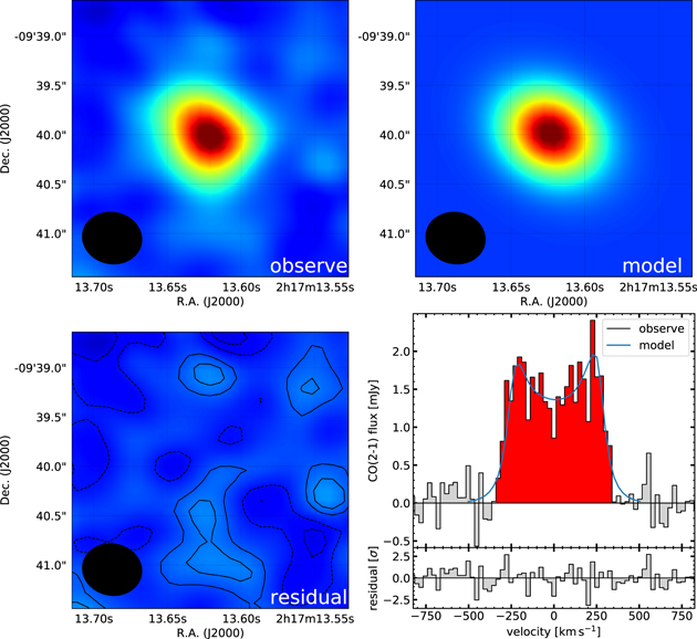
Figure 6. Top left: observed integrated intensity map of CO(2–1). The filled black ellipse in the bottom left corner shows the synthesized beam size. Top right and bottom left: Same as top left, but for the best-fit model through GalPaK3D and residual (observed − model), respectively. The contours in the residual map represent −2σ, −σ, σ, and 2σ. Bottom right: observed and modeled line profiles (red and blue solid curve, respectively). The residual normalized with 1σ noise level is shown in the lower part.
Download figure:
Standard image High-resolution imageTable 3. Best-fit Parameters Derived by GalPaK3D
| flux (Jy km s−1) | 1.10 ± 0.05 |
| r1/2 (kpc) a | 2.30 ± 0.12 |
| inclination (deg) | 47.6 ± 6.5 |
| PA (deg) | 42.8 ± 2.0 |
| rt (kpc) b | 0.48 ± 0.22 |
 c
c
| 350 ± 30 |
Notes. Uncertainties are estimated based on simulations (see text).
a Half-light radius. b Turnover radius. c Inclination-corrected maximum rotational velocity.Download table as: ASCIITypeset image
4.2. Stellar Distribution
In order to derive properties of the stellar distribution, we fit Sérsic profile models to HST WFC3/IR J125 and H160-band images using GALFIT (Peng et al. 2002). GALFIT is a program code that fits a given surface brightness model convolved with a PSF to an observed galaxy. Four (six) bright but unsaturated stars in the J125 (H160) image of the CANDELS-UDS field are stacked to construct the PSFs for the fittings. The ∼25 × 25 boxy region centered at the image peak is used for the fitting. The pixels contaminated by neighboring objects are masked out. After sky subtraction, we first fit the surface brightness with a single-component Sérsic profile. The fitting parameters are the central position, the total magnitude, the half-light radius (R1/2), the Sérsic index (n), the axial ratio, and the position angle. We also fit another surface brightness model with two-component Sérsic profiles. In this fitting, Sérsic indices are fixed to be n = 4 for the bulge and 1 for the disk because the galaxy has a rotating gas disk and seems to consist of the bulge and disk in the HST composite image (see Figure 1). The fitting parameters are the total magnitude of each component, the half-light radius of each component (R1/2;bulge, R1/2;disk), and the axial ratio of the bulge. The central position of each component, the position angle of each component, and the axial ratio of the disk are fixed to the values derived from the single-component fitting. The derived best-fit parameters are listed in Table 4. The observed and fitted radial profiles are shown in Figure 7.
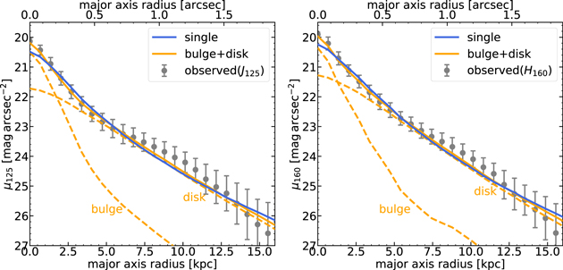
Figure 7. Left: J125 radial profiles of SXDS1_13015. μ125 is the surface brightness. Gray circles with error bars show the observed radial profile. The best-fit single-component model and two-component (bulge + disk) model are shown with the blue and orange solid line, respectively. Dashed orange lines show the bulge and disk components of the best-fit two-component model. Right: same as the left panel, but for H160.
Download figure:
Standard image High-resolution imageTable 4. Results of Fitting Sérsic Profile Models to J125 and H160 Images
| Filter | J125 | H160 |
|---|---|---|
| n a | 2.04 ± 0.19 | 1.76 ± 0.11 |
| R1/2 (kpc) a | 3.54 ± 0.15 | 3.22 ± 0.07 |
| b/a a | 0.62 ± 0.01 | 0.60 ± 0.01 |
| PA (deg) a | 32.0 ± 0.9 | 36.2 ± 0.7 |
| R1/2;bulge (kpc) b | 0.45 ± 0.23 | 0.44 ± 0.22 |
| R1/2;disk (kpc) b | 5.05 ± 0.33 | 4.49 ± 0.21 |
| Lbulge/Ldisk b |

|

|
Notes. Uncertainties are estimated by changing the sky level within its error, stars to construct the PSFs, and the size of the fitting region.
a Results of the single-component fitting. Sérsic index, half-light radius, axis ratio, and position angle, respectively. b Results of the two-component (bulge (n = 4) and disk (n = 1)) fitting.Download table as: ASCIITypeset image
Assuming a constant mass-to-luminosity ratio, we derived the stellar mass surface density profile of SXDS1_13015 from the J125 distribution modeled with the single-component model. In Figure 8 the derived profile of SXDS1_13015 is plotted with the median profiles of galaxies at different redshifts by Patel et al. (2013). The sample galaxies of Patel et al. (2013) are selected at a constant cumulative number density of 1.4 × 10⁻⁴ Mpc−3 for different redshifts (corresponding to a stellar mass of ∼1.1 × 10¹¹ M☉ for 1.0 < z < 1.5). The number of sample galaxies at 1.0 < z < 1.5 is 20 (∼65% of them are quiescent galaxies). The surface density profiles are derived by assuming a constant mass-to-luminosity ratio, and they are modeled by fitting a single-component Sérsic profile to the rest-frame optical image for each redshift using GALFIT. The standard deviations for the median profiles at z ∼ 1.0–1.5 and z ∼ 1.5–2.0 are calculated by generating 1000 median profiles based on the uncertainties of the median half-light radius and Sérsic index at each redshift provided by Patel et al. (2013). SXDS1_13015 shows a slightly higher surface density than the median of the galaxies at similar redshift, and it reaches a surface density comparable to that of galaxies at z ∼ 0.06. The surface density of SXDS1_13015 is also comparable to that of local galaxies with the stellar mass of the Milky Way (van Dokkum et al. 2013). At r ≲ 1 kpc, the surface density of SXDS1_13015 is lower than those of the median profiles. However, the scale of 1 kpc is comparable to the HWHM of the PSF for our fitting (∼0.8 kpc ∼ 1.5 pixels), and it is possible that the profile is not sufficiently recovered within this scale.
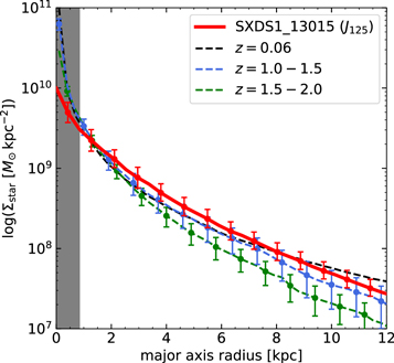
Figure 8. The red line shows the stellar mass surface density profile of SXDS1_13015 with the uncertainty derived from the error of the stellar mass and galaxy parameters of GALFIT. A constant mass-to-luminosity ratio is assumed. The green, blue, and black dashed lines show the median profiles of galaxies at z = 1.5–2.0, 1.0–1.5, and 0.06, respectively (Patel et al. 2013). The galaxies are selected at a constant cumulative number density of 1.4 × 10⁻⁴ Mpc−3 for different redshifts (corresponding to the stellar mass of ∼1.1 × 10¹¹ M☉ for 1.0 < z < 1.5). We show the standard deviation of each median profile (see text). The gray shaded region shows the HWHM of PSFs for our fitting.
Download figure:
Standard image High-resolution image4.3. Molecular Gas and Stellar Distribution in SXDS1_13015
4.3.1. Modeled Gas and Stellar Distributions
By using the modeled molecular gas distribution derived by GalPaK3D and the stellar distribution derived by GALFIT, we obtain intrinsic radial surface distributions of the molecular gas as well as the stellar component in SXDS1_13015 (Figure 9). The uncertainty on the molecular gas surface distribution is estimated with radial profiles derived from GalPaK3D fitting to the 100 simulated cubes (see Section 4.1.3). The uncertainty on the stellar surface distribution is derived from uncertainties on the total stellar mass and galaxy parameters of GALFIT. We also derive the gas-mass fraction (fgas) at each radius. The uncertainty on fgas is derived from the uncertainties on the molecular gas and stellar radial surface distributions. fgas is higher than the total galactic value (∼0.55) at r ≲ 3 kpc, and it decreases with increasing galactocentric radius from ∼0.6 at the central region to ∼0.2 at ∼ 3 × r1/2. The molecular gas is distributed farther inside the galaxy than the stars and seems to be associated with the bulge rather than the stellar disk, which is also indicated by the best-fit half-light radii.
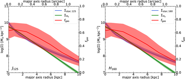
Figure 9. Left: modeled (intrinsic) molecular gas and stellar (J125) radial distributions of SXDS1_13015. The green and blue line show the molecular gas and stellar (one component) surface density profile, respectively. The shaded regions show the uncertainties. The gas-mass fraction (fgas = Mmol/(Mmol + Mstar)) is also plotted with the red line, and the shaded region shows the uncertainty on fgas. Right: same as the left panel, but for H160.
Download figure:
Standard image High-resolution imageBy using the best-fit kinematic parameters of the molecular gas disk, dynamical masses ( ) at r = r1/2, 2r1/2, 3r1/2 (r1/2 is half-light radius of molecular gas disk) are estimated to be ∼(0.7, 1.3, 2.0) × 1011
M☉. We also derive the molecular gas and stellar masses within these radii assuming that the inner mass (m( < r)) is proportional to the luminosity within the radius (L( < r)) in the J125 image,
) at r = r1/2, 2r1/2, 3r1/2 (r1/2 is half-light radius of molecular gas disk) are estimated to be ∼(0.7, 1.3, 2.0) × 1011
M☉. We also derive the molecular gas and stellar masses within these radii assuming that the inner mass (m( < r)) is proportional to the luminosity within the radius (L( < r)) in the J125 image,

The molecular gas and stellar masses within r = r1/2, 2r1/2, 3r1/2 are mmol ∼ (0.7, 1.2, 1.4) × 1011 M☉ and mstar ∼ (0.4, 0.7, 0.9) × 1011 M☉, respectively. Baryon fractions (fbaryon = (mmol + mstar)/(Mdyn + mmol + mstar)) within these radii are estimated to be ∼ 0.61, 0.59, and 0.53 within r = 3r1/2 ∼ 7 kpc.
4.3.2. CO and Optical Half-light Radii
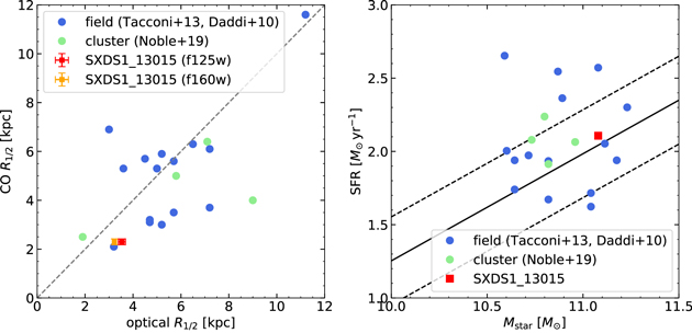
Figure 10 (left) shows the location of SXDS1_13015 in the optical versus CO half-light radius plane compared to other field and cluster galaxies at z ∼ 1–1.6. The field sample includes the 12 main-sequence galaxies at z ∼ 1–1.5 by Tacconi et al. (2013) and the 3 sBzK galaxies by Daddi et al. (2010). All galaxies of the field sample show both disk-like morphologies in HST images and clear CO velocity gradients (classified as "Disk(A)" by Tacconi et al. (2013)). The CO and optical half-light radii were estimated by fitting an n = 1 Sérsic profile to the image planes or circular Gaussians to the uv planes, and by fitting a single Sérsic profile to HST-WFC3 I814 band data using GALFIT, respectively. The typical uncertainties on both CO and the optical half-light radius are ∼25%. The cluster sample consists of the 4 cluster galaxies at z ∼ 1.6 by Noble et al. (2019) (J0225-371, J0225-460, J0225-281, and J0225-541); they are detected with high S/Ns and show clear velocity gradients in CO(2–1). The CO and optical half-light radii were estimated by fitting elliptical Gaussians to the CO(2–1) images and a single Sérsic profile to H160-band data using GALFIT, respectively. The typical uncertainty on the CO half-light radius is ∼10%. As shown in Figure 10 (right), the field and cluster sample galaxies are mostly main-sequence galaxies at a similar redshift and with a similar stellar mass to SXDS1_13015.
Figure 10. Left: distribution of the galaxies in the optical vs. CO half-light radius plane. SXDS1_13015, field galaxies, and cluster galaxies are shown as red and orange squares, blue circles, and green circles, respectively. For SXDS1_13015, the results of the single-component fit to J125 and H160 images are plotted in red and orange, respectively. The field galaxies are taken from Tacconi et al. (2013) and Daddi et al. (2010; classified "Disk(A)" in Tacconi et al. (2013)). The cluster galaxies are taken from Noble et al. (2019; with a high S/N and clear velocity gradient in CO(2–1)). The dashed line shows optical equals to CO. Right: stellar mass vs. SFR. SXDS1_13015, field galaxies, and cluster galaxies are shown in red, blue, and green, respectively. The main sequence at z = 1.5 (Speagle et al. 2014) is shown with a solid line together with the scatter (dashed lines). The difference of the adopted IMF is corrected with the factor by Speagle et al. (2014).
Download figure:
Standard image High-resolution image
Studies in rest-frame V band of galaxies at similar redshift to SXDS1_13015 show that SFGs with similar stellar mass show a half-light radius of a few to a few dozen kiloparsec and a Sérsic index of n ∼ 1.5−4 (e.g., Wuyts et al. 2011; van der Wel et al. 2014; Shibuya et al. 2015; Mowla et al. 2019). The n and half-light radius of SXDS1_13015 derived from the single-component fitting are within the range of those obtained in other main-sequence galaxies. The CO and optical half-light radii of SXDS1_13015 are, however, relatively small as compared with other main-sequence galaxies, but the half-light radius of the CO-to-optical ratio of SXDS1_13015 (R1/2,CO/R1/2,F125W = 0.65 ± 0.04, R1/2,CO/R1/2,F160W = 0.71 ± 0.04) is typical in these samples.
5. Summary
We presented the results of subarcsecond ALMA 12 CO(2–1) and 12 CO(5–4) observations toward a massive main-sequence galaxy at z = 1.45 (SXDS1_13015). These observations enabled us to study molecular gas properties, its distribution in the galaxy, and the CO(5–4)/CO(2–1) flux ratio in a UV clump detected in the rest-frame UV HST image. By fitting a rotating-gas disk model to the CO(2–1) data, we derived the molecular gas distribution and kinematics. Combining this with the HST images, we compared the properties of molecular gas and stellar distributions. The results are as follows:
- (i)CO(2–1) and CO(5–4) emission lines are clearly detected from the galaxy (Figure 2), and the symmetric and double-peak line profile of CO(2–1) implies the presence of the molecular gas disk in the galaxy. R52 of the galaxy is 1.1 ± 0.2, which suggests that the CO excitation ladder of the galaxy is similar to that of the Milky Way rather than to that of sBzK galaxies at z ∼ 1.5. The molecular gas mass of the galaxy is 1.45 × 10¹¹ M⊙, adopting R21 = 1 (the Milky Way value) and a metallicity-dependent CO-to-H2 conversion factor. The gas-mass fraction and depletion time are 0.55 ± 0.08 and 1.1 ± 0.3 Gyr, respectively.
- (ii)In the R52 map (Figure 3), the peak value of R52 is ∼2.2, comparable to that of the average of sBzK galaxies at z ∼ 1.5. R52 peaks at the position of the UV clump. These results are similar to a result of a hydrodynamic simulation of a clumpy galaxy (Bournaud et al. 2015). In the UV clump, the gas density and/or temperature are/is higher than those in the other galactic regions.
- (iii)By using GalPaK3D, the molecular gas distribution of the galaxy traced by CO(2–1) is well represented by the rotating-disk model (Figure 6). The half-light radius of the modeled gas disk is 2.3 kpc.
- (iv)When we compare the molecular gas distribution and stellar distribution derived by fitting Sérsic models to the rest-frame optical HST images, the molecular gas is more concentrated in the galactic center (Figure 9). The gas-mass fraction decreases with increasing galactocentric radius from ∼0.6 at the central region to ∼0.2 at ∼3 × r1/2, suggesting that the galaxy is forming its bulge.
We thank the anonymous referee for useful comments and suggestions that improved the paper. We are grateful to K. Nakanishi, F. Egusa, K. Saigo, and the staff at the ALMA Regional Center for their help with the data reduction. We also thank K. Tadaki for his critical comment on our earlier study of this galaxy. F.M. is supported by a Research Fellowship for Young Scientists from the Japan Society of the Promotion of Science (JSPS). K.O. is supported by JSPS KAKENHI grant No. JP19K03928. This paper makes use of the following ALMA data: ADS/JAO.ALMA#2015.1.01129.S. and #2011.0.00648.S. ALMA is a partnership of ESO (representing its member states), NSF (USA) and NINS (Japan), together with NRC (Canada), MOST and ASIAA (Taiwan), and KASI (Republic of Korea), in cooperation with the Republic of Chile. The Joint ALMA Observatory is operated by ESO, AUI/NRAO and NAOJ.
Software: GALFIT (Peng et al. 2002), GalPaK3D (Bouché et al. 2015), CASA (v4.7.2; McMullin et al. 2007).
Footnotes
- 4
- 5
- 6
Generally, the HWHM of a two-dimensional Gaussian corresponds to the half-light radius.