


Abstract
Recently, we developed the correlation-aided reconstruction (CORAR) method to reconstruct solar wind inhomogeneous structures, or transients, using dual-view white-light images. This method is proved to be useful for studying the morphological and dynamical properties of transients like blobs and coronal mass ejection (CME), but the accuracy of the reconstruction may be affected by the separation angle between the two spacecrafts. Based on the dual-view CME events from the Heliospheric Imager CME Join Catalogue in the Heliospheric Cataloguing, Analysis and Techniques Service (HELCATS) project, we study the quality of the reconstruction of CME using the CORAR method under different STEREO stereoscopic angles. We find that when the separation angle of the spacecraft is around 150°, most CME events can be well reconstructed. If the collinear effect is considered, the optimal separation angle should locate between 120° and 150°. Compared with the direction of the CME given in the Heliospheric Imager Geometrical Catalogue from HELCATS, the parameters of the CME obtained by the CORAR method are reasonable. However, the CORAR-obtained directions deviate toward the meridian plane in longitude, and toward the equatorial plane in latitude. An empirical formula is proposed to correct these deviations. This study provides the basis for the configuration of the spacecraft of our recently proposed Solar Ring mission concept.
Export citation and abstract BibTeX RIS
1. Introduction
Since the 1990s, many spacecrafts have been launched for observing various solar phenomena. One of the most solar eruptions of interest is the coronal mass ejection (CME), which injects a large amount of magnetized plasma from the corona into the heliosphere and creates major disturbances in the interplanetary medium. CMEs propagating toward Earth may couple with the Earth's magnetosphere and trigger magnetic storms (Gosling et al. 1990), bringing about difficulties in the operation of space-borne and ground-based instruments, causing potential problems for modern communications. To better understand CMEs, instruments for in situ measurements of their interplanetary signatures and remote sensing observations of their origins at/near the Sun are required. In particular, white-light observations by coronagraphs and heliospheric cameras are essential to study the morphological and dynamical properties of CMEs in three-dimensional (3D) space, e.g., the Large Angle and Spectrometric Coronagraph (Brueckner et al. 1995) on board the Solar and Heliospheric Observatory (Domingo et al. 1995), the Solar Mass Ejection Imager (Eyles et al. 2003), the coronagraphs (COR-1 and COR-2), and heliospheric imagers (H i-1 and H i-2; Harrison et al. 2005) in the SECCHI suite (Howard et al. 2008) on board the Solar Terrestrial Relations Observatory (STEREO; Kaiser et al. 2008), the Wide-field Imager for Solar Probe on board the Parker Solar Probe (Fox et al. 2016), and the coronagraph Multi Element Telescope for Imaging and Spectroscopy (METIS) and heliospheric imager SoloHi on board the Solar Orbiter (Muller et al. 2013).
Based on multi-view observations, the directions of the propagation and the velocities of solar wind transients can be calculated by comparing the tracks on the time-elongation profiles, i.e., the J-maps (Sheeley et al. 1999), from different vantage points. For CMEs with sophisticated structures, some geometrical models with different assumptions are developed to obtain the kinematic parameters of CMEs. Such forward modeling techniques include the cone or ice-cream cone models (Zhao et al. 2002; Xie et al. 2004; Xue et al. 2005; Zhao 2008), the self-similar expansion (SSE) model (Davies et al. 2012, 2013; Wang et al. 2013; Volpes & Bothmer 2015), and especially the Graduated Cylindrical Shell model (Thernisien et al. 2006, 2009; Thernisien 2011). Compared with these modeling methods, the geometric localization method (Pizzo & Biesecker 2004; de Koning et al. 2009) can reproduce the 3D shapes of CMEs by triangulating the boundary of imaging CMEs without a prior model. This was further improved by the "mask fitting" method (Feng et al. 2012, 2013), which corrects the CME shapes in accordance with images from three different points. For single-perspective polarized Thomson-scattering images, the polarization ratio technique (Moran & Davila 2004; Dere et al. 2005; Moran et al. 2010; Susino et al. 2014) can locate the center of mass along the line of sight (LOS) and thus generate a density distribution. Multi-view observations may improve the accuracy of the results from the polarimetric method. Considering the correlation between the same CME patterns from different vantage points, the local correlation tracking method (Mierla et al. 2009, 2010; Feng et al. 2013) calculates the correlation coefficients between images from different perspectives to determine the 3D structure representing CMEs. Recently, Li et al. (2018, 2020) successfully developed the so-called correlation-aided reconstruction (CORAR) method to recognize and determine the location, angular size, and directions of the propagation of solar wind transients in 3D space by using STEREO H i-1 images from two perspectives.
Different methods based on multi-view observations may require different optimal stereoscopic angles for the best results. de Koning et al. (2009) found that the geometric localization method works best when the separation angle of the spacecraft is between 30° and 150°. For the tie-pointing technique, the error in the reconstruction is inversely correlated with the base angle between the two STEREO spacecrafts (Mierla et al. 2010, 2011). Liewer et al. (2011) also studied the tie-pointing and triangulation method, which gives reliable results on the directions of the propagation of the CME when the stereoscopic angle is within 50°. The local correlation tracking plus triangulation method works well for small separation angles (Mierla et al. 2009), but does a poor job for large separation angles (Feng et al. 2013). Our previous work studied the 3D reconstruction of small-scale transients by the CORAR method with simulated blobs, and concluded that a dual-spacecraft angle of about 120° is the most suitable scheme for the CORAR technique (Lyu et al. 2020). However, different from blobs, CMEs are large-scale structures. This should be studied if the best separation angle of the two spacecrafts for more complicated CMEs is the same or similar to our previous work. Thus, in this paper, we apply the CORAR technique to the observed CMEs by H i-1 to achieve the optimal stereoscopic angle for large-scale heliospheric transients. In Section 2, we introduce the CORAR method and H i-1 data for the reconstruction, as well as an assessment and classification of the quality of the reconstruction and the effect of collinearity. Section 3 analyzes the goodness of the reconstruction in different angular intervals to achieve the optimal stereoscopic angle, and derives the deviations or errors from the directions of the propagation of the CME, which are further discussed in Section 4. Finally, we provide our conclusions in Section 5.
2. Data and Method
We use the CORAR method to process the H i-1 Level 2 white-light images from 2008 December to 2012 February for 3D reconstruction. During the interval, the two spacecrafts STEREO A and B moved away from each other at the speed of about 22° per yr, with their separation angle (the angle between two spacecrafts bisected approximately by the Sun–Earth line) increasing from about 85°–225°. The field of view (FOV) from the H i-1 cameras is 20° × 20°, observing the area from 4° to 24° outward from the Sun. The pixel resolution of the H i-1 images is 1024 × 1024, and the time interval between two successive images is 40 minutes, showing the evolution of fine structures in solar wind transients. Before the reconstruction, the H i-1 images were processed by removing starlight and noise, and the pixel shifts of continuous images were corrected for running difference.
Compared with other manual approaches for locating CME features, the CORAR method can automatically recognize the patterns belonging to the same transient in dual-view images. After data preprocessing, the selected images in the same time period are projected on 81 meridian planes from −80° to 80° in longitude of the Heliocentric Earth Ecliptic (HEE) coordinate, with the grid resolution of 1° in latitude from −80° to 80° and 0.4 solar radii (R⊙) in the radial direction. Then, the program calculates the distribution of cc, which is the Pearson correlation coefficient between the projections of the dual images and is further corrected by the local signal-noise ratios, to present the 3D structures of CMEs. The size of the sampling box searching for CME patterns during the cc calculation is 11 × 21 × 5, representing 10° in latitude, 8R⊙ in radial distance, and 160 minutes with five time steps, respectively. To save storage, we only stored effective cc data with values higher than the threshold of 0.5, which is considered as the high-cc region to match solar wind transients. More details of the CORAR process can be found in Li et al. (2020).
We use the CMEs listed in the Heliospheric Imager CME Join Catalogue (HIJoinCAT), as well as their kinematic properties in the Heliospheric Imager Geometrical Catalogue (HIGeoCAT; Barnes et al. 2019), to achieve our goal in this study. These two catalogs are both generated by the Heliospheric Cataloguing, Analysis and Techniques (HELCATS; Plotnikov et al. 2016; Harrison et al. 2018; Murray et al. 2018; Barnes et al. 2019; Pluta et al. 2019) project funded under the European Union's Seventh Framework Programme for Research and Technological Development. HIJoinCAT contains the manually observational CME events simultaneously detected by two H i cameras since 2007, and HIGeoCAT provides their kinematic properties, including the directions and speeds of the propagation, estimated by using the Fixed-Phi (FP), Harmonic-Mean (HM), and SSE techniques. During the period of interest, HIJoinCAT lists 198 CME events. But we find that images of three events are missing or damaged, and therefore exclude them. Then the other 195 events are classified into three levels based on the performance of the CORAR reconstruction (see Figure 1), by visual inspection of the completeness and distortion. For the events at Level 1, the high-cc regions are disorganized and appear as scattered dots or small parts. They do not reflect the characteristics of a CME at all, but just show many pieces. At Level 2, the high-cc regions are not as fragmented Level 1 events and propagate outward with time. They can be recognized as parts of a CME. In most cases, these parts belong to the fronts or leading edges of CMEs. For these events, we think that the CMEs are recognized but the quality is not good enough. The well-reconstructed events are classified as Level 3. In this case, the propagating high-cc regions almost cover the whole CME.
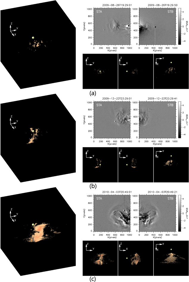
Figure 1. Panel (a): the H i-1 images and the presentation of the reconstruction in the HEE coordinate of the 2009 August 26 CME event at the Level 1 quality of reconstruction. Panel (b): 2009 December 22 CME event at the Level 2 quality of reconstruction. Panel (c): 2010 April 3 CME event at the Level 3 quality of reconstruction.
Download figure:
Standard image High-resolution imageBesides, the "collinear effect," which can cause fake high-cc regions near the connecting line of two spacecrafts, should be noted (Li et al. 2018; Lyu et al. 2020). Here, the collinear effect in the reconstruction of CMEs is also assessed and categorized into three levels by visual inspection (see Figure 2): the events at Level 1 are severely affected by the collinear effect, resulting in an artificial high-cc region extending along the connecting line; for the events at Level 2, the collinear effect results in the presence of an unreal structure, but real CME patterns can still be identified; for the events at Level 3, the reconstruction is not influenced by the collinear effect. The number of CME events at these levels are summarized in Table 1. The CME events at Level 2 or 3 of both the performance and the collinear effect are included in the following analysis of the optimal separation angle of the STEREO spacecraft, resulting in a total of 165 events; 156 of them have kinematic properties in HIGeoCAT fitted by STEREO A or B data, while 14 have results only from one spacecraft. The classification of the collinear effect is used to find CME events unsuitable for CORAR reconstruction, and the performance of the reconstruction is classified to determine the optimal angle.
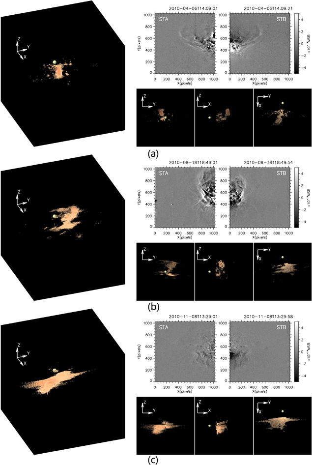
Figure 2. Panel (a): the H i-1 images and the presentation of the reconstruction in the HEE coordinate of the 2010 April 6 CME event at Level 3 of the collinear effect. Panel (b): the 2010 August 18 CME event at Level 2 of the collinear effect. Panel (c): the 2010 November 8 CME event at Level 1 of the collinear effect.
Download figure:
Standard image High-resolution imageTable 1. The Number and Proportion of Events at Each Level
| Level 1 | Level 2 | Level 3 | |
|---|---|---|---|
| Performance of the reconstruction | 10 (5.1%) | 71 (36.4%) | 114 (58.5%) |
| Collinear effect | 20 (10.2%) | 44 (22.6%) | 131 (67.2%) |
Download table as: ASCIITypeset image
3. Results
We obtained the optimal stereoscopy for CORAR according to the 3D performance of the reconstruction of CMEs in the heliosphere. Figure 3 shows the proportions of events at three levels of the collinear effect in panel (a) and of the quality of the reconstruction in panel (b) as a function of the separation angle, as well as a histogram of the total number of dual-view CME events studied. The errors are estimated by  , where p is the proportion and n is the number of events in each interval. Since the events in 2008–2009 are scarcer than those after that time period, the first two angle intervals are set at 85°–115° and 115°–135° to increase the number of events for statistical analysis, and the subsequent intervals are 10°. Note that most of the CME events were observed when the separation angle was near 180°. This possibly resulted from the increasing common space near the Thomson spheres (DeForest et al. 2013; Howard & DeForest 2012; Howard et al. 2013) of the two cameras, which makes it easier to recognize the same CME from two perspectives. When the angle is larger or smaller than 180°, the LOS from two observers tend to be perpendicular, observing different two-dimensional features of the same optically thin transient. Meanwhile, the time period selected for our study belongs to the ascending phase of Solar Cycle 24, so the frequency of the CME increases as the separation angle increases over time. The data plotted in Figure 3(b) excludes CME events at Level 1 of the collinear effect.

Figure 3. Panel (a): the proportions of CME events with error bars at different levels of the collinear effect as a function of the separation angle. Events with angles of 85°–115° and 205°–225° are at Level 3. Panel (b): the proportions of CME events at different levels of performance of the reconstruction, without events at Level 1 of the collinear effect. The number of CME events in each angle interval is plotted in light blue bars.
Download figure:
Standard image High-resolution imageFrom Figure 3(a), the proportion of CME events without the collinear effect is less than 30% when the separation angle is between 145° and 175°, especially more than 50% of events suffer from a severe collinear effect in the 155°–175° interval. Therefore, most events during this period are considered unsuitable for the CORAR reconstruction and excluded from the following analysis. There are few CME events at the Level 1 quality of reconstruction as shown in Figure 3(b), especially no events between 115° and 185°. This indicates that the dual-view CMEs can be recognized easily according to the CORAR reconstruction over the selected range of angles. With a larger or smaller separation angle, it is less likely to leave common features of a CME on the dual images, leading to an increase in Level 1 events. For events at the Level 2 and Level 3 performance of reconstruction, the proportion of curves have different tendencies: the Level 3 profile reaches the maximum at 145°–155° and has the local minimum at 155°–165°, while the case for Level 2 is the opposite. More than 85% of events between 135° and 155° are reconstructed well, implying similar features to a CME left completely in the dual-perspective images. In the range of 155°–175°, the nearly parallel LOS from two observers bring about a severe collinear effect. Although we exclude bad events, almost half of the effective CME events are at the Level 2 quality of reconstruction. Around 180°, the proportion of Level 3 events rises to 0.74, and decreases monotonously as the separation angle gets larger, with more CMEs partially reconstructed. In summary, when the stereoscopic angle is 150° ± 5°, most CME events are well reconstructed, even if influenced to some extent by the collinear effect. On the other hand, when the stereoscopic angle is around 120°, the collinear effect is minimized with all the qualities of reconstruction at Level 2 or 3. The compromise between the two factors suggests that the optimal separation angle of the two spacecrafts should locate between 120° and 150°. This result is similar to that of our previous study (Lyu et al. 2020), in which the separation angle of 120° is concluded to be the best one.
To discuss the accuracy of the location of CMEs, we select effective CME events at Level 2 or Level 3 of the reconstruction quality and the collinear effect to track the 3D trajectories of the reconstructed CMEs. Assuming that CMEs move in the radial direction, we calculate the cc-weighted center of a CME, and take the average position in longitude and latitude during its propagation as its direction. The cc-weighted longitude φ and latitude θ are calculated as follows:
where φi and θi are the latitude and longitude of any point in the high-cc region. Figure 4 compares the directions of the CME propagation in the Heliocentric Earth Equatorial (HEEQ) Coordinate system obtained by the CORAR method and by the SSE-fitting technique (Davies et al. 2012) with a fixed 30° half width from HIGeoCAT. The calculated correlation coefficient r larger than 0 indicates a positive correlation between the CORAR and SSE parameters. Meanwhile, taking the SSE parameters as the independent variable, we can obtain linear fits with positive slopes (black lines in Figure 4), implying the accuracy of the direction obtained by the CORAR method. If there was a perfect agreement, the slope should be unity. Compared with the single-view SSE parameters, the averages from two spacecrafts may be more precise. This can partially explain the larger correlation coefficients and the slopes of the fitting lines in Figures 4(c) and (f) than those in the other panels. However, as the SSE longitude of CME events increases, the increasing magnitude of the CORAR longitude is significantly smaller, revealed by the fitting slopes generally below 0.5. One possible explanation is that the SSE longitude recorded in HIGeoCAT is fitted for the apex of the CME instead of the whole CME, and fitting errors may come from the single-view fitting methods and the CORAR reconstruction method. Nevertheless, this phenomenon possibly reflects a clear deviation toward the meridian plane in longitude for the reconstructed CMEs by CORAR. It is more intuitive in Figure 5, which shows the difference between CORAR and SSE values. It is apparent that the deviation in longitude increases with the absolute longitude.

Figure 4. A comparison of the fitting longitude (panels (a)–(c)) and latitude (panels (d)–(f)) in the HEEQ coordinate from the CORAR method and from the SSE model, with the fitting profiles of all CORAR results as a function of the SSE results (black lines). The correlation coefficient r, the fitting functions as well as the coefficients of determination R2 are listed. The horizontal axes represent the SSE longitude and latitude, and the vertical axes represent the parameters obtained by the CORAR method. The SSE results are fitted from STEREO A images in panels (a) and (d) and from STEREO B images in panels (b) and (e). The SSE results in panels (c) and (f) are mean values from STEREO A and B. The CME events at the Level 3 quality of reconstruction are marked in green, and events at Level 2 in red.
Download figure:
Standard image High-resolution image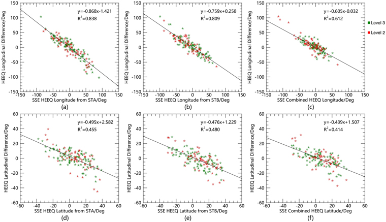
Figure 5. The errors between CORAR and SSE longitudes φCORAR − φSSE (panels (a)–(c)) and latitudes θCORAR − θSSE (panels (d)–(f)) in the HEEQ coordinate, and their fitting profiles (black lines). The fitting functions and the coefficients of determination R2 are listed. The horizontal axes represent the SSE longitude and latitude, and the vertical axes represent the CORAR results minus the SSE results. The SSE results are fitted from STEREO A images in panels (a) and (d) and from STEREO B images in panels (b) and (e). The SSE results in panels (c) and (f) are mean values from STEREO A and B. The CME events at the Level 3 quality of reconstruction are marked in green, and events at Level 2 in red.
Download figure:
Standard image High-resolution imageIn the direction of the latitude, the correlations between CORAR and SSE values are relatively stronger, and the fitting slopes in Figures 4(d)–(f) are closer to 1 than those in longitude, but there are deviations toward the equatorial plane, similar to the longitudinal deviations (see Figures 5(d)–(f)). The deviations may be related to the unphysical structures caused by the intrinsic defects of the triangulation method. A specific analysis is discussed in the next section. A large uncertainty may exist when using CORAR methods to locate CMEs with different scales and morphologies in the same direction of the propagation, because our CORAR method does not incorporate any morphological assumptions and takes the irregular structures of reconstructed CMEs for tracking trajectories. The HIGeoCAT catalog also provides the kinetic parameters of the CMEs obtained from two other fitting models: the FP model and HM model, which are considered as extreme cases of the SSE with half widths of 0° and 90°, respectively (Davies et al. 2012; Moestl & Davies 2013). Since the comparison of the values from the two fitting models and from our CORAR method is similar to the analysis above, the details are not described here.
Based on the above comparative analysis, we try to correct the direction of the CMEs obtained by the CORAR method. Since the deviation may depend on the separation angle of the spacecraft, we use piecewise functions to make the correction, as shown in Figure 6. Note that when the separation angle ranges from approximately 135° to 175°, the connecting line of the two spacecrafts basically exists in the common H i-1 FOV, so that the collinear effect is serious (Figure 3(a)). Meanwhile, this angular interval also contains the most suitable separation angle for a good reconstruction. Therefore, we divide the function interval into three: 85°–135°, 135°–175°, and 175°–225°. We take the CORAR parameters as the independent variable to linearly fit the average values from the single-view fitting models in HIGeoCAT, and get the empirical formulas for the correction of CORAR values as follows:
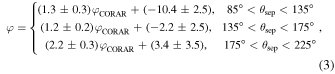
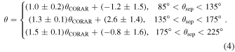
θsep is the separation angle, and φCORAR (θCORAR) and φ (θ) are the initial and corrected HEEQ longitude (latitude) obtained by the CORAR method, respectively. The fitting method is different from those used in Figures 4 and 5, considering both errors from the CORAR and modeling results. The CORAR errors measure the possible deviations of reconstructed CMEs from the average directions of propagation, and the errors of the modeling results are standard deviations of six values from three single-view techniques by fitting STEREO A and B images. The slopes of the correction lines for the HEEQ longitude and latitude are slightly larger than 1 when θsep < 175°. Above this range, the slopes of the correction formulas are apparently larger than 1, especially in longitude. This may result from the increase of events at the Level 2 quality of reconstruction, with their partial structures in smaller absolute longitude and latitude reconstructed better. This indicates that a separation angle larger than 180° may not be suitable for the reconstruction of CMEs by the CORAR method.

Figure 6. The fitting lines for the correction of the directions obtained from CORAR in the HEEQ longitude (panels (a)–(c)) and latitude (panels (d)–(f)) with the separation angle of 85°–135° (panels (a) and (d)), 135°–175° (panels (b) and (e)), and 175°–225° (panels (c) and (f)).
Download figure:
Standard image High-resolution image4. Discussion
Mierla et al. (2010) demonstrated that there are many factors that affect the quality of the reconstruction and the accuracy of the location for 3D reconstruction methods, which can be roughly divided into observational errors and methodical errors. For the CORAR method, the possible errors may arise from three aspects. First, similar features of the same 3D structure cannot be observed from dual perspectives, so the reconstruction cannot be performed. Second, similar patterns that do not belong to the same transients are mistaken for real structures, thus the reconstruction contains unreal transients. Third, similar features of the same structure can be observed in dual-view images, but fail to be reconstructed completely due to factors like too large sizes of the sampling box or grid cells. The first type is common for reconstruction methods based on multi-view observations, especially when the separation angle of the spacecraft is close to 90°. From different LOSs for the Thomson-scattering integral, the same transient may have completely different patterns, so that the errors are difficult to deal with. Considering that the characteristics of large-scale transients can be sufficiently recognized in detail based on the high resolution of H i-1 images and the control parameters can be adjusted, the third type of error is easy to control. As for the second type of error, it may be theoretically estimated and further corrected.
To analyze the second type of error, we apply a simple spherical model to simulate the 195 CME events, as shown in Figure 7. The SSE-fitting parameters of the corresponding CME event are assumed as the actual direction of the CME for the spherical model. The radial distance from the Sun is determined by the instantaneous position of the reconstructed CME from the CORAR method, and the spherical radius is determined by the half width of the reconstructed CME in latitude. The blue area is theoretically the space containing all possibly reconstructed structures in the common FOV, assuming a homogeneous distribution. To estimate the influence of these false structures, we calculate the cc-weighted center of this area so that its deviation from the center of the initial model can be obtained, as shown in Figure 8. The existence of these false structures causes the calculated directions of CMEs to shift toward the meridian plane in longitude and the equatorial plane in latitude, which is more serious for CME events with larger characteristic scales. Especially, CME events with a half width larger than 30° may produce an angular deviation of more than 10° in longitude and latitude. Furthermore, we subtract the aforementioned errors from the CORAR parameters for each CME event in Figure 4, which are shown in Figure 9. After subtracting the calculated systematic errors, the slopes of the fitting lines for the CORAR latitude and longitude approach to unity, and the correlation coefficient r and the statistical measure R2 generally increase. In particular, Figures 9(c) and (f) show fitting lines with slopes near 1 and a positive correlation larger than 0.8 for average SSE parameters. However, the corrected fitting straight lines are still less than 1. Although the single-view fitting parameters cannot be regarded as the real directions of the CME, the theoretical deviation cannot fully explain the deviation from the CORAR method shown in Figures 4 and 5. Note that the blue space in Figure 5 is an extremely ideal case. In reality, the reconstructed transients may only occupy small parts of the blue space, or even scattered points for CME events at the Level 1 performance of reconstruction. The spherical model is too simple to fit complex solar wind structures. In addition, other solar wind transients existing in the observation images, such as blobs or successive CMEs, may generate structures outside the blue space. Finally, this error analysis requires that the cc distribution, which can measure the authenticity of the reconstructed inhomogeneous transient, is approximately uniform, but this is not true for most CME events. More work is needed to analyze the source of the deviation in further detail for complete error correction.
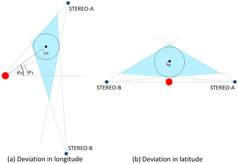
Figure 7. The principle of systematic errors modeled by a spherical shell in longitude and latitude. Panel (a): the model observed along the Z-axis in the HEE coordinate. Panel (b): the model observed along the Sun–Earth line. The red ball represents the Sun and the two blue balls mark the two STEREO spacecrafts. The black and blue point represent the center of the CME model and the blue area, respectively.
Download figure:
Standard image High-resolution image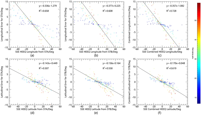
Figure 8. The systematic errors in the HEEQ longitude (panels (a)–(c)) and latitude (panels (d)–(f)) calculated by a simple spherical model for the CME events, with the fitting lines in black. The horizontal axes represent SSE-fitting longitude and latitude, and the vertical axes represent the theoretical errors. The SSE results are fitted from STEREO A data in panels (a) and (d) and from STEREO B data in panels (b) and (e). The SSE results in panels (c) and (f) are the mean values of those from STEREO A and B. The color bar represents the latitudinal half width of CME events.
Download figure:
Standard image High-resolution image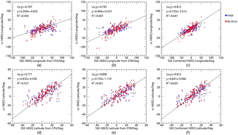
Figure 9. The CORAR-calculated longitude (panels (a)–(c)) and latitude (panels (d)–(f)) corrected by systematic error in Figure 8, as well as their fitting lines (black lines). The correlation coefficient r, the fitting functions as well as the coefficients of determination R2 are listed. The horizontal axes represent the SSE-fitting results, and the vertical axes represent the CORAR results minus errors (red) and those without error correction (blue). The SSE results are fitted from STEREO A data in panels (a) and (d) and from STEREO B data in panels (b) and (e). The SSE results in panels (c) and (f) are mean values from STEREO A and B.
Download figure:
Standard image High-resolution image
5. Conclusion
In our previous work (Lyu et al. 2020), we studied the 3D reconstruction of small-scale blobs by the CORAR method, and discussed the optimal stereoscopic angle for the Solar Ring mission (Wang et al. 2020, 2021). In this study, we use the CORAR method to reconstruct H i-1 dual-perspective images from 2008 December to 2012 February, obtain the 3D cc distribution to study the performance of the reconstruction of CME events in the heliosphere, and calculate the direction of transients. The CME events studied are from the HIJoinCAT catalog in the HICATS project, which consists of dual-view CME events, so that the theoretical 3D reconstruction is ensured.
We find that the influence of the collinear effect clashes with the variation of the quality of the reconstruction as the separation angle increases: when the stereoscopic angle rises from 90° to 180°, the patterns of the CMEs in the dual-perspective images may be more similar, suitable for CORAR reconstruction; at the same time, the spacecrafts appear in the FOV of each other, resulting in difficulty in locating the accurate position of CMEs in the direction of the connecting line and resulting in large-scale fake structures. Among the angular intervals, 120°–150° is considered as suitable for the reconstruction of CMEs. Within 145°–155°, some CME events are influenced by the collinear effect, but most cases are well reconstructed. When the separation angle is smaller, the proportion of CME events with a good quality of reconstruction decreases, while the collinear effect weakens until 115°. Below this range, CMEs may fail to be reconstructed. As the separation angle gets larger than 155°, the influence of the collinear effect becomes more serious so that a considerable amount of CME events are not reconstructed well.
We also calculate the directions of CMEs in the HEEQ coordinate and compare them with the single-view fitting results from the HIGeoCAT catalog, so as to correct the CORAR results by fitted empirical formulas in different angle intervals. We prove that the CORAR results are positively correlated with the SSE-fitting results, while apparent deviations toward the meridian plane in longitude and smaller shifts toward the equatorial plane in latitude exist. We speculate that the reason for the deviations is mainly due to the unreal structure produced by the similar characteristics of different CME patterns. For further discussion, we use a simple spherical model to calculate the theoretical error for each CME event. It can partially explain the sources of the deviation and improve the CORAR prediction of CME directions. To completely analyze and correct this deviation, distinguish the difference between the real and unreal structures, and realize absolute reconstruction for various solar wind inhomogeneous transients, further research is needed in the future.
Our work supports the spacecraft scheme of the Solar Ring mission (Wang et al. 2020). In this plan, the separation angles among the six spacecrafts orbiting the Sun have the values of 120° and 150°. According to our studies, the 120° scheme is suitable for small-scale transients, and the 150° scheme can work for large-scale CMEs. We hope our work can be helpful for the design of this mission as well as other mission concepts for solar wind observations in the future.
We acknowledge the use of the data from STEREO/SECCHI, which are produced by the consortium of RAL (UK), NRL (USA), LMSAL (USA), GSFC (USA), MPS (Germany), CSL (Belgium), IOTA (France), and IAS (France). The SECCHI data can be found in the STEREO Science Center (https://stereo-ssc.nascom.nasa.gov/data/ins_data/secchi_hi/L2/). We also acknowledge the service provided by the data repository at National Space Science Data Center (http://www.nssdc.ac.cn/eng/), where our data products are stored. This work is supported by the Strategic Priority Programs of the Chinese Academy of Sciences (XDB41000000 and XDA15017300), the National Natural Science Foundation of China (41774178, 41761134088, 41804161, and 42074222), and the fundamental research funds for the central universities (WK2080000077). Y.W. is particularly grateful for the support of the Tencent Foundation.