


Abstract
HectoMAP is a dense, red-selected redshift survey to a limiting r = 21.3 mag covering 55 deg2 in a contiguous 1 5 strip across the northern sky. This region is also covered by the Subaru/Hyper Suprime-Cam (HSC) Subaru Strategic Program photometric survey enabling a range of applications that combine a dense foreground redshift survey with both strong and weak lensing maps. The median redshift of HectoMAP exceeds 0.3 throughout the survey region, and the mean density of the redshift survey is ∼2000 galaxies deg−2. Here we report a total of 17,313 redshifts in a first data release covering 8.7 deg2. We include the derived quantities Dn4000 and stellar mass for nearly all of the objects. Among these galaxies, 8117 constitute a 79% complete red-selected subsample with r ≤ 20.5 mag, and an additional 4318 constitute a 68% complete red-selected subsample with 20.5 < r(mag) < 21.3. As examples of the strengths of HectoMAP data, we discuss two applications: refined membership of redMaPPer photometrically selected clusters and a test of HSC photometric redshifts. We highlight a remarkable redMaPPer strong lensing system. The comparison of photometric redshifts with spectroscopic redshifts in a dense survey uncovers subtle systematic issues in the photometric redshifts.
1. Introduction
Redshift surveys are a pillar of modern cosmology. They chart the way galaxies mark the distribution of matter in the universe on large scales and they hold clues to the way individual galaxies and systems of galaxies evolve.
Beginning in the 1980s, digital detector technology enabled advances in the extent and quality of redshift surveys (e.g., Davis et al. 1982; Geller & Huchra 1989; Shectman et al. 1996). Over the last 25 years, wide-field multiobject spectrographs have enabled a fantastic array of surveys that cover large regions of the universe at relatively recent epochs (e.g., Strauss et al. 2002; Colless et al. 2003; Ahn et al. 2014; Alam et al. 2015; Liske et al. 2015; Drinkwater et al. 2018) and probe the universe at redshifts z > 1 (e.g., Lilly et al. 2009; Newman et al. 2013; Silverman et al. 2015; Scodeggio et al. 2018). The next decade promises even more spectacular advances with more heavily multiplexed systems, for example, the Dark Energy Spectroscopic Instrument survey (DESI Collaboration et al. 2016), 4MOST (Finoguenov et al. 2019), MOONRISE (Maiolino et al. 2020), Maunakea Survey Explorer (Percival et al. 2019), and Subaru/Prime Focus Spectograph (Tamura et al. 2018).
Hectospec, a 300-fiber wide-field instrument on the 6.5 m MMT, has played an important role in redshift surveys of galaxies covering the most recent 7 Gyr of the history of the universe (Kochanek et al. 2012; Geller et al. 2014, 2016; Zahid et al. 2016). The SHELS survey (Geller et al. 2005, 2010) was the first to combine a foreground dense redshift survey with a weak lensing map to explore the combined power of these modern cosmological tools (see also Geller et al. 2014; Hwang et al. 2016).
The SHELS survey (Geller et al. 2016), complete to an extinction-corrected R = 20.2 mag over roughly 8 deg2, also provides a benchmark for more extensive color-selected surveys. An MMT survey of the COSMOS field, hCOSMOS, provides additional photometric and spectroscopic calibration (Damjanov et al. 2018).
HectoMAP, carried out with Hectospec on the MMT, is a red-selected redshift survey covering 55 deg2 to a limiting r = 21.3 mag in a narrow strip across the northern sky. The Subaru/Hyper Suprime-Cam (HSC) Subaru Strategic Program (SSP) (Aihara et al. 2018) also covers the HectoMAP region with deep five-band photometry. Here we describe the first data release (HectoMAP DR1) for the HectoMAP survey covering 8.7 deg2 of the survey. This region of the HectoMAP DR1 includes the region covered by the HSC SSP public DR1.
The average density of HectoMAP is ∼2000 galaxies per square degree. This high density is the signature property of the redshift survey that underlies its central scientific goals (Geller & Hwang 2015). These goals include identification and characterization of clusters (e.g., Sohn et al. 2018a, 2018b) and voids (Hwang et al. 2016) throughout the survey region. Because massive clusters accrete roughly half of their mass from a redshift of 0.5 to the present, the HectoMAP survey serves as a baseline for dynamical measures of cluster accretion history.
The powerful combination of HSC SSP imaging and HectoMAP is a foundation for exploring the way galaxies trace the large-scale matter distribution by combining a weak lensing map with the foreground redshift survey. The combined data also provide a host of strong lensing candidate systems from individual massive galaxies to massive clusters of galaxies.
The HectoMAP survey fills an interesting niche for enhanced understanding of the evolution of the quiescent galaxy population and its dependence on environment. Damjanov et al. (2019) use SHELS data for 4200 quiescent objects to investigate relationships among stellar mass, size, and stellar population age to redshift z ∼ 0.6. HectoMAP DR1 contains nearly 12,000 quiescent objects, and the entire HectoMAP survey will contain ∼70,000 for more extensive investigations in this redshift range. The density, completeness, and deep HSC photometry of the final HectoMAP sample will enable insights into the dependence of quiescent galaxy size evolution on environment (e.g., Damjanov et al. 2015; Gargiulo et al. 2019).
We provide a redshift, Dn 4000, and stellar mass for a total of 17,313 galaxies in the 8.7 deg2 HectoMAP DR1 region. Among these, there are 9775 galaxies in highly complete red subsamples of galaxies with r < 21.3 mag. Section 2 includes discussion of the Sloan Digital Sky Survey (SDSS) and Subaru HSC photometry, the spectroscopy, the derived parameters Dn 4000 and stellar mass, the completeness of the survey, and the redshift distribution. We highlight two direct applications in Section 3. Section 3.1 extends our earlier investigations of redMaPPer (RM) clusters; Section 3.2 demonstrates the power of HectoMAP for investigation of subtle systematics in photometric redshifts. We use cosmological parameters Ωm = 0.3, ΩΛ = 0.7, and H0 = 70 km s−1 Mpc−1 throughout.
2. The Data
HectoMAP is a dense redshift survey with a median redshift ∼0.3. The average number density of galaxies with spectroscopic redshifts is ∼2000 deg−2 (∼1200 galaxies deg−2 within the highly complete red-selected subsample Geller et al. 2011; Geller & Hwang 2015; Hwang et al. 2016; Sohn et al. 2018a, 2018b). The selection for the complete HectoMAP sample is (g − r)model,0 > 1 for rpetro,0 ≤ 20.5 mag; for 20.5 < rpetro,0 (mag) ≤ 21.3 we include an additional constraint, (r − i)model,0 > 0.5. Here, rpetro,0 refers to the SDSS Petrosian magnitude corrected for foreground extinction. The SDSS model colors, (g − r)model,0 and (r − i)model,0, are also corrected for foreground extinction. Hereafter we designate r = rpetro,0, (g − r) = (g − r)model,0, and (r − i) = (r − i)model,0 in the text; we retain the full notation in the figure captions for clarity.
The full HectoMAP survey covers 54.64 deg2 within the boundaries 200 < R.A. (deg) < 250 and 42.5 < decl. (deg) < 44.0. Here we include redshifts, stellar masses, and Dn 4000 for galaxies in the region 242 < R.A. (deg) < 250 and 42.5 < decl. (deg) < 44.0, an area of 8.7 deg2 that includes the HSC SSP public DR1 region (Aihara et al. 2018). The median redshift for HectoMAP in this data release is z = 0.31. Hereafter we refer to this data release as HectoMAP DR1. Figure 1 shows the location of HectoMAP on the sky.
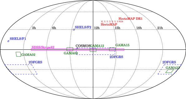
Figure 1. Redshift survey coverage in equatorial coordinates. Red squares indicate the HectoMAP redshift survey. The locations of some other example spectroscopic surveys are also displayed: 2DFGRS (Colless et al. 2003), SDSS/Stripe82 (Abazajian et al. 2009), GAMA (Liske et al. 2015), COSMOS (Lilly et al. 2009), and SHELS/F1 and F2 (Geller et al. 2016). The sky coverage of the SDSS spectroscopic survey can be found here: https://www.sdss.org/wp-content/uploads/2015/01/dr12_legacy_plus_segue_coverage.png.
Download figure:
Standard image High-resolution imageIn 2009 we observed the GTO2deg2 field (Miyazaki et al. 2007) as a test of the feasibility of the HectoMAP project. We acquired 4405 redshifts (out of 4541) with Hectospec covering this 2.1 deg2 field (Kurtz et al. 2012), which overlaps slightly with HectoMAP DR1. The original selection for red objects in this region was (r − i) > 0.4 throughout the apparent magnitude range, r < 21.3 mag. In the full HectoMAP survey we have no (r − i) cut for galaxies with r ≤ 20.5 mag and a tighter (r − i) > 0.5 for objects with apparent magnitudes between 20.5 and 21.3.
We reduced the Hectospec spectroscopy in the GTO2deg2 field (Kurtz et al. 2012) with an IRAF-based pipeline (Kurtz & Mink 1998) including the RVSAO cross-correlation package (Kurtz & Mink 1998). We have rereduced these data with the current pipeline, HSRED v2.0; we include the rereduced results for the 505 galaxies in the small overlap region here. There is essentially no difference between the redshifts returned by the two pipelines. We discuss the overall HectoMAP sample selection based on SDSS photometry (Section 2.1), the available HSC photometry (Section 2.2), and the MMT Hectospec spectroscopy (Section 2.3). We discuss the completeness of the survey and the redshift distribution in Section 2.4. Sections 2.5 and 2.6 include descriptions of the parameters we derive from the spectroscopy: Dn 4000 and stellar mass.
2.1. SDSS Photometry
The SDSS provides the photometric basis for HectoMAP. Because observations for HectoMAP extend over 10 yr, we used the SDSS data releases beginning with DR7 (Abazajian et al. 2009) and progressing to DR9 (Ahn et al. 2012). We have now updated all of the catalogs to SDSS DR16 (Ahumada et al. 2020), the basis for all of the quantities quoted here.
The primary HectoMAP survey targets are red galaxies with (g − r) > 1.0 for r ≤ 20.5 mag (the bright red subsample) and galaxies with 20.5 < r(mag) ≤ 21.3, (g − r) > 1 and (r − i) > 0.5 (the faint red subsample). We select galaxies based on the SDSS probPSF = 0, where probPSF is the probability that the object is a star. The color cut for the faint red sample removes the galaxies with z ≲ 0.2; the cut is necessary because the observing time required without it is prohibitive. For both the bright and faint subsamples we remove low surface brightness objects that are generally beyond the limits of the MMT spectroscopy by requiring rfiber,0 < 22.0 mag. Table 1 lists the number of photometric objects in the entire sample and in various subsamples.
Table 1. Number of Galaxies in Subsamples
| Subsample | Nphot | Nspec,Hecto a | Nspec,SDSS b | Nspec,NED c | Nspec,total d | Completeness (%) |
|---|---|---|---|---|---|---|
| Entire Sample (r ≤ 23.0) | ⋯ | 14767 | 2409 | 137 | 17313 | ⋯ |
| Supplementary (21.3 < r ≤ 23.0) | ⋯ | 1083 | 384 | 0 | 1467 | ⋯ |
| Main (r ≤ 21.3) | 41006 | 13684 | 2025 | 137 | 15846 | 38.6 |
| Main (g − r > 1.0, r ≤ 21.3) | 20526 | 11509 | 1441 | 43 | 12993 | 63.3 |
| Main (g − r > 1.0, r − i > 0.5, r ≤ 21.3) | 12164 | 8561 | 1211 | 3 | 9775 | 80.4 |
| Main (g − r ≤ 1.0) | 20480 | 2175 | 584 | 94 | 2853 | 13.9 |
| Bright (r ≤ 20.5) | 20076 | 9015 | 1590 | 135 | 10740 | 53.5 |
| Bright (g − r > 1.0) | 10305 | 7051 | 1023 | 43 | 8117 | 78.8 |
| Bright (g − r > 1.0, r − i > 0.5) | 5837 | 4660 | 794 | 3 | 5457 | 93.5 |
| Bright (g − r ≤ 1.0) | 9771 | 1964 | 567 | 92 | 2623 | 26.8 |
| Faint | 20930 | 4669 | 435 | 2 | 5106 | 24.4 |
| Faint (g − r > 1.0) | 10221 | 4458 | 418 | 0 | 4876 | 47.7 |
| Faint (g − r > 1.0, r − i > 0.5) | 6327 | 3901 | 417 | 0 | 4318 | 68.2 |
| Faint (g − r ≤ 1.0) | 10709 | 211 | 17 | 2 | 230 | 2.1 |
Notes.
a Number of spectroscopic redshifts from MMT/Hectospec. b Number of spectroscopic redshifts from SDSS and BOSS. c Number of spectroscopic redshifts from NASA Extragalactic Database including Gronwall et al. (2004), Jaffé et al. (2013). d Total number of spectroscopic redshifts.Download table as: ASCIITypeset image
Figure 2(a) shows the color–magnitude diagram for HectoMAP DR1 galaxies. The contours show all photometric galaxies in the field, and the red squares mark the spectroscopic targets with redshifts (Section 2.3). In Figure 2(b), the filled and open histograms display the r-band magnitude distributions for galaxies with (g − r) > 1.0 and for those with (g − r) > 1.0 and rfiber < 22 mag, respectively. More than 92% of the galaxies with (g − r) > 1.0 and r ≤ 21.3 mag, the main targets of the redshift survey, are rfiber < 22 mag. The HectoMAP DR1 completeness quoted below refers to completeness above our explicit limiting surface brightness.
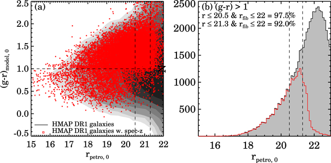
Figure 2. (a) Color–magnitude (g − r vs. r) diagram for galaxies in the HectoMAP DR1 region. Red squares show the galaxies with spectroscopic redshifts. The horizontal line indicates the color selection limit, (g − r) = 1. The vertical lines show the magnitude selections of r = 20.5 mag and r = 21.3 mag, respectively. We apply the (r − i) > 0.5 selection for selecting targets in between the two vertical lines. (b) The r-band magnitude distribution for HectoMAP DR1 galaxies with (g − r) > 1 (black filled histogram) and those with (g − r) > 1 and rfiber < 22 mag (red open histogram).
Download figure:
Standard image High-resolution image2.2. HSC Photometry
The HectoMAP region is included in the Wide portion of the Subaru/HSC (Miyazaki et al. 2012) SSP. The first public HSC SSP data release (Aihara et al. 2018) includes 4.7 deg2 of the HectoMAP region. Figure 3 shows the HectoMAP DR1 region, 242 < R.A. (deg) < 250 and 42.5 < decl. (deg) < 44.0, along with the 4.7 deg2 footprint of the included HSC SSP DR1 (red points). The total area covered by the HectoMAP release is 8.7 deg2.
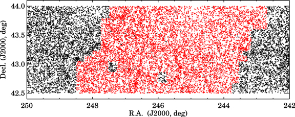
Figure 3. HectoMAP DR1 footprint. Black points are galaxies with spectra in the HectoMAP DR1. Red points are galaxies with photometric counterparts in the HSC SSP DR1 catalog. Note the two significant islands of black within the red patch where HSC data are missing.
Download figure:
Standard image High-resolution imageThe HSC Wide photometry includes data in g, r, i, z, and y to 5σ depths of 26.8, 26.4, 26.2, 25.4, and 24.7 mag, respectively, for point sources. Because our main goal is to provide spectroscopic data and because our observations were based on SDSS photometry, we do not use the HSC photometry explicitly here.
There are two sizeable missing patches (black islands in Figure 3) in the HectoMAP HSC DR1 region in all bands. Aihara et al. (2018) also highlight several general issues that affect the relatively bright (i < 19 mag) galaxies in HectoMAP. For example, some galaxies in the HectoMAP magnitude range are shredded, and most galaxies with i < 19 mag have composite model magnitudes inconsistent with the SDSS.
We take advantage of the public release of photometric redshifts in the HSC SSP public DR2 (Aihara et al. 2019). Here we use HSC SSP DR2 because it provides photometric redshifts for galaxies in the entire HectoMAP DR1 region. Tanaka et al. (2018) derive photometric redshifts based on a variety of techniques ranging from classical template-fitting to machine-learning techniques. They test these techniques against available spectroscopy. Although the test samples used by Tanaka et al. (2018) are large, they emphasize the need for additional dense, complete, independent spectroscopic data. HectoMAP DR1 is much shallower than the HSC SSP data, but the density and completeness of the spectroscopy over its depth and area are unique. We discuss the HSC photometric redshifts in Section 3.2.
2.3. Hectospec Spectroscopy
We measured redshifts with the 300-fiber Hectospec mounted on the MMT 6.5 m telescope (Fabricant et al. 2005) from 2009 to 2019. Hectospec deploys 300 fibers over a 1° diameter field of view and covers the wavelength range of 3700–9100 Å. The standard total exposure time for a HectoMAP observation is 1 hour in three 20-minute segments to enable cosmic-ray removal. In good conditions a single Hectospec observation returns ∼250 redshifts. The typical yield is ∼200 reliable redshifts.
Obtaining a uniformly complete redshift survey over the large HectoMAP field is a major observational challenge. To position Hectospec for each run, we first evaluated the spectroscopic completeness of the survey at the beginning of the run in 0.25° × 0.25° pixels. We then ranked the pixels from the least to most complete. Finally, we chose a set of Hectospec positions that maximized coverage of the highly ranked (most incomplete) pixels. Variable observing conditions affected the yield for each position. Over the 10-year survey we revisited each position in the entire survey ∼10 times. In the DR1 region, the typical number of revisits is ∼9.
It is not always possible to fill all of the Hectospec fibers with survey targets. We used the remaining fibers to observe bluer objects prioritized by apparent magnitude (brighter objects without a redshift had higher priority). This approach yielded 2205 Hectospec redshifts for unique objects bluer than the survey selection limits (Table 1).
Figure 4 shows three absorption line spectra (panels (a)–(c)) for galaxies at z ∼ 0.25 covering the range of the cross-correlation quality measure, RXC (Tonry & Davis 1979). In all cases the H and K break is apparent. These absorption line objects are the main focus of HectoMAP. In the lower right panel (d) we show an emission line spectrum at lower redshift; the object has negligible continuum and strong lines.
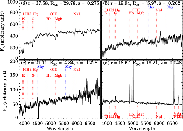
Figure 4. Sample spectra for galaxies in the HectoMAP DR1 region.
Download figure:
Standard image High-resolution imageWe show the spectra for a fixed window in the rest frame. The variation in the quality of the spectra is driven largely by observing conditions including lunar phase (for the bright portion of the survey), seeing, and transparency. The pipeline provides a standard indicator of the quality of the spectrum, RXC, a measure of the significance of the cross-correlation peak (Tonry & Davis 1979).
Figure 5 shows RXC as a function of extinction-corrected r. We show the distribution of RXC for galaxies with a redshift derived from an absorption line template (red points) and for galaxies with redshifts derived from an emission line template (blue points). The emission line templates are overrepresented among the brightest and faintest galaxies and among galaxies with the highest and lowest RXC. At bright apparent magnitudes we sample relatively more blue objects; at the faintest magnitudes, objects with strong emission lines are more likely to yield a reliable redshift (e.g., Glazebrook et al. 2007). At the lowest RXC, we identify objects with a reliable redshift by visual inspection. The presence of more than one emission line makes the visual identification more likely. The highest RXCs reflect the presence of strong emission lines (see the example in Figure 4).
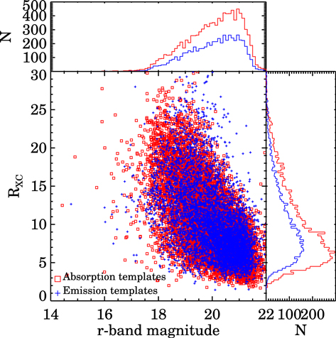
Figure 5. RXC from RVSAO as a function of rpetro,0. Red and blue points show redshifts derived from emission and absorption line spectral templates, respectively. The histograms display rpetro,0 and RXC distributions for emission (blue) and absorption (red) line redshifts.
Download figure:
Standard image High-resolution imageAlthough we could use RXC alone to select reliable redshifts, we inspect each spectrum visually after the pipeline processing. Visual inspection recovers or discards (1) spectra with badly subtracted night sky lines, (2) spectra where there are two objects at different redshifts in the same fiber aperture, and (3) active galactic nuclei and quasars that do not match the templates. On the basis of the visual inspection we classify objects as “Q” for high quality, “?” for doubtful cases, and “X” for complete failures. We conservatively report a redshift only for a spectrum classified as Q.
Table 1 lists the number of photometric objects in various color and magnitude ranges (main, bright red, faint red, blue). For each sample in the table, we list the number of unique Hectospec spectra with Qs (column 3) and the additional number of unique objects from the combination of SDSS and BOSS in each sample (column 4). Column 5 lists the number of reliable redshifts in each subsample. In some cases this number exceeds the sum of columns 3 and 4 because we include a small number of redshifts from the NASA Extragalactic Database (NED, including Gronwall et al. 2004; Jaffé et al. 2013). We highlight (boldface) the sample and subsamples where we strive for completeness within the magnitude and color limits. Although we select extended sources with probPSF = 0, 524 objects turn out to be stars. In other words, among the objects with Q quality spectra, ∼3% are actually stars listed in the Appendix. Thus the estimates of completeness based on the sets of photometric SDSS extended objects (Table 1) are probably slight underestimates because some fraction of the remaining objects are also stars.
Table 2 compiles the 17313 HectoMAP DR1 redshifts. Among the galaxies in Table 2, 1467 are fainter than r = 21.3 mag. These faint objects account for the excess relative to the 15,846 objects in Table 1, which reviews the main survey targets. We include the SDSS ID (column 1), the R.A. and decl. (columns 2 and 3), the SDSS r, (g − r), and (r − i) (columns 4–6), the redshift with its error (column 7), the source of the redshift (column 8), the stellar mass and Dn 4000 (columns 9 and 10), and an RM cluster membership indicator (column 11). The error in the redshift in column 8 is the formal error returned by cross correlation. The median formal error is 28 km s−1; (24 km s−1 and 31 km s−1 for emission and absorption line spectra, respectively).
Table 2. HectoMAP DR1 Catalog
| SDSS Object ID | R.A. | Decl. | rpetro,0 | (g − r) a | (r − i) a | z | z Source | Ma | Dn 4000 | redMaPPer |
|---|---|---|---|---|---|---|---|---|---|---|
| 1237659326027596446 | 243.530137 | 42.506127 | 20.56 ± 0.11 | 1.66 | 0.54 | 0.31258 ± 0.00029 | MMT |

| 2.17 ± 0.24 | ⋯ |
| 1237659326564205123 | 243.530863 | 43.202909 | 20.00 ± 0.17 | 0.81 | 0.09 | 0.13372 ± 0.00002 | MMT |

| 1.12 ± 0.03 | ⋯ |
| 1237659327100945547 | 243.531558 | 43.757552 | 21.33 ± 0.08 | 1.98 | 1.01 | 0.74919 ± 0.00026 | BOSS |

| 1.54 ± 0.09 | ⋯ |
| 1237659327100945058 | 243.531600 | 43.778505 | 20.53 ± 0.04 | 1.56 | 0.78 | 0.49998 ± 0.00021 | MMT |

| 1.52 ± 0.05 | ⋯ |
| 1237659326564205607 | 243.531601 | 43.259037 | 20.42 ± 0.13 | 0.94 | 0.45 | 0.25664 ± 0.00012 | MMT |

| 1.67 ± 0.05 | HMRM05629 |
Note.
a Foreground extinction-corrected model colors.Only a portion of this table is shown here to demonstrate its form and content. A machine-readable version of the full table is available.
Download table as: DataTypeset image
An earlier Hectospec redshift survey, SHELS, provides a measure of the internal error based on a set of repeat measurements intended for this purpose (Geller et al. 2014). SHELS is composed of two fields, F1 and F2. In the F2 field a set of repeat measurements for 1651 unique objects provides the internal estimate (normalized by (1 + z)); for emission line objects the internal error is 24 km s−1, and for absorption line objects (the bulk of the HectoMAP sample) the internal error is 48 km s−1. In their Hectospec survey of the COSMOS field based on the same observing protocols followed for HectoMAP, Damjanov et al. (2019) obtain similar internal errors for emission and absorption line redshifts, 26 km s−1 and 42 km s−1, respectively. It is interesting that these internal errors are essentially identical to the XCSAO estimate for emission line objects but that they exceed it by about 50% for absorption line spectra.
As a measure of the external error, Figure 6 examines the HectoMAP DR1 overlap with SDSS/BOSS. There are 129 and 852 objects with Hectospec observations that overlap SDSS and BOSS observations, respectively. Figure 6(a) compares redshifts from SDSS/BOSS and Hectospec. Figure 6(b) shows redshift differences in the rest frame. The black histogram in Figure 6(b) shows the distribution of redshift differences (Δc(zSDSS/BOSS − zHecto)/(1 + zHecto)) between Hectospec and SDSS (or BOSS) for all overlaps. We derive the best-fit Gaussian for this distribution (dashed curve). The mean and standard deviation for the total overlapping sample are 39 km s−1 and 44 km s−1, respectively. There is a small systematic offset of 39 km s−1 between Hectospec and SDSS/BOSS redshifts in the sense that Hectospec redshifts are slightly larger, but this offset is comparable to the 1σ standard deviation, 44 km s−1. We note that the offset is somewhat smaller at low redshift: Δc(zSDSS/BOSS − zHecto/(1 + zHecto)) = 26 ± 32 km s−1 at z < 0.15. However, the fraction of HectoMAP DR1 galaxies with z < 0.15 is only ∼10%.
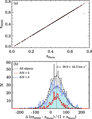
Figure 6. (a) Comparison between Hectospec and SDSS/BOSS redshifts for galaxies with overlapping measurements in the HectoMAP DR1 region. (b) Distributions of the redshift differences for the same objects. The black filled histogram shows all objects with both Hectospec and SDSS/BOSS redshifts. Red open and blue hatched histograms show spectra with high signal to noise (S/N > 5) or low S/N, respectively. The dashed curves show the best-fit Gaussians for each distribution. The vertical dotted line indicates the Gaussian mean for the entire sample (black histogram).
Download figure:
Standard image High-resolution imageWe also plot redshift differences for overlapping objects with high (red histogram) and low (blue histogram) S/N Hectospec spectra in Figure 6. Both distributions are well represented by Gaussians. The best-fit Gaussian mean and standard deviation for the high S/N and low S/N overlapping samples are 38 ± 29 km s−1 and 40 ± 51 km s−1, respectively. The mean redshift offset between Hectospec and SDSS/BOSS is insensitive to the S/N of the Hectospec spectra; the external error increases with decreasing S/N as expected. Damjanov et al. (2018) use 2661 overlapping objects to find that Hectospec redshifts exceed their zCOSMOS counterparts by a small zero-point offset of 17 ± 2 km s−1.
The small systematic offsets between HectoMAP and SDSS/BOSS and between Hectospec and zCOSMOS redshifts are comparable with or less than the 1σ error in HectoMAP redshifts based on the sum in quadrature of the internal and external errors. In fact, for the entire HectoMAP sample, the external error alone (Figure 6) slightly exceeds the systematic shift. We used both XCSAO and template fitting applied to the data and to a set of simulated spectra to try to identify the source of these systematics, but the tests failed to reveal the underlying, fundamental cause. Because these small systematics are irrelevant for most applications of the survey, we simply summarize them here for completeness.
2.4. Survey Completeness and Redshift Distribution
The upper panel of Figure 7 shows the differential completeness of the redshift survey as a function of r for the entire DR1 and for subsamples segregated by (g − r) (see Table 1). We made no attempt to obtain a complete blue sample ((g − r) < 1). We show the curve merely to indicate the content of the data set. The differential completeness of the red-selected (g − r) ≥ 1 subsample exceeds ∼75% for r < 20 and drops to 50% for r < 20.9.
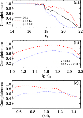
Figure 7. (a) Spectroscopic survey differential completeness as a function of rpetro,0. Solid, dashed, and dotted lines show the completeness for all, red ((g − r)model,0 ≥ 1.0), and blue ((g − r)model,0 < 1.0) galaxies. (b) Survey completeness as a function of (g − r)model,0 for the bright (rpetro,0 ≤ 20.5 mag) and faint (20.5 < rpetro,0(mag) ≤ 21.3) subsamples. (c) Same as (b) but as a function of (r − i)model,0.
Download figure:
Standard image High-resolution imageDense redshift surveys that overlap the redshift range of HectoMAP include the 2dF Galaxy Redshift Survey (Colless et al. 2001, 2003), SDSS/BOSS (Ahn et al. 2014; Alam et al. 2015), GAMA (Liske et al. 2015), and SHELS (Geller et al. 2016). The 2dF survey obtained redshifts for ∼250,000 objects brighter than bJ = 19.45 mag over ∼2000 deg2 of the sky; the typical survey density is ∼150 galaxies deg−2. The SDSS Main Galaxy sample (Strauss et al. 2002) is ≳94% complete to a limiting r = 17.77 mag over a large region with a typical density ∼70 galaxies deg−2; there is no color selection. BOSS (Ahn et al. 2014; Alam et al. 2015) covers the magnitude range, but it is color selected and sparse (see Figure 10 below). GAMA (Liske et al. 2015) covers about 5.5 times the area of HectoMAP to a limiting r = 19.8 in five regions of the sky (Figure 1). The completeness of GAMA generally exceeds 94%, and there is no color selection. The typical density of GAMA is ∼1000 galaxies deg−2. Finally, SHELS covers ∼8 deg2 with a completeness ≳94% to R ∼ 20.2 mag (r ∼ 20.5 mag) with an average density ∼2000 galaxies deg−2 in two well-separated fields. The depth is comparable to the bright portion of HectoMAP, and there is no color selection. The set of overlapping surveys with no color selection provides a basis for assessing the impact on scientific results resulting from the red color selection in HectoMAP.
Figures 7(b) and (c) show the fractional completeness of the r ≤ 20.5 mag (red dashed line) and the 20.5 < r(mag) ≤ 21.3 (blue dotted line) subsamples of HectoMAP as a function of (g − r) (b) and (r − i) (c). For the faint subsample, the completeness declines for lower values of (g − r) as a result of the cut in (r − i). In the brighter portion with r ≤ 20.5 mag, the completeness also declines for bluer (g − r) because we initially prioritized galaxies with (r − i) > 0.5 (Hwang et al. 2016; Sohn et al. 2018a, 2018b). In general, the completeness declines for the reddest galaxies because they are at redshifts ≳0.5 and thus tend to be faint, lower surface brightness objects (see Figure 1 of Hwang et al. 2016).
Figure 8(a) shows the completeness of the red-selected sample with r ≤ 20.5 mag as a function of position on the sky. The bins are 025 × 025. The completeness is remarkably uniform (>80%). Only 15% of the pixels are less than 70% complete; there are no pixels with a completeness <50%.
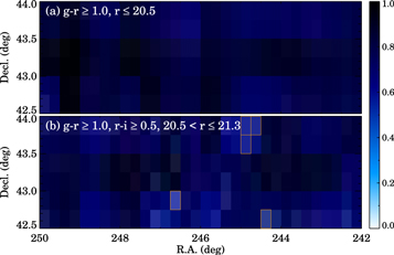
Figure 8. (a) Survey completeness in 025 × 025 pixels for red-selected galaxies with rpetro,0 ≤ 20.5 mag in HectoMAP DR1. Darker colors indicate more complete pixels. (b) Survey completeness as in (a) but for red-selected objects with 20.5 < rpetro,0(mag) < 21.3 mag.
Download figure:
Standard image High-resolution imageFigure 8(b) shows the completeness on the sky for red-selected galaxies with 20.5 < r ≤ 21.3 mag. For this magnitude range there is an (r − i) selection in addition to the constraint (g − r) ≥ 1. Only 29% of the pixels are less than 70% complete; 5% of the pixels have a completeness less than 50%. The fainter portion of HectoMAP is less complete because of the greater sensitivity to observing conditions. In particular, the observations are more sensitive to seeing. The survey is also less complete near the decl. boundaries where observations are inefficient.
Figure 9 shows the redshift distribution for the HectoMAP DR1 sample and for two subsamples segregated by (g − r). In each panel, the blue hashed histogram shows redshifts from SDSS/BOSS. From the upper to lower panel, the median redshifts are ∼0.31, ∼0.36, and ∼0.16, respectively.
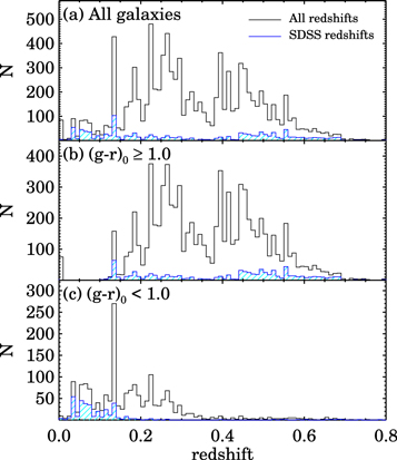
Figure 9. Redshift distribution for HectoMAP DR1 (open histogram): (a) all galaxies, (b) (g − r)model,0 ≥ 1.0, and (c) (g − r)model,0 < 1.0. Blue hatched histograms show the corresponding SDSS/BOSS redshift distributions.
Download figure:
Standard image High-resolution imageThe sharply defined peaks are the signature of the large-scale structure of the universe. It is striking that the peaks appear clustered over broad redshift ranges. The low-density region in the redshift range ∼ 0.30–0.38 is remarkable. The spatial scale corresponding to this deficit is an impressive ∼290 Mpc in the radial direction. This scale is comparable to the largest HectoMAP void found by Hwang et al. (2016) (see their Figure 16). Voids with this extent occupy a long tail in the N-body simulations explored by Hwang et al. (2016).
Figure 10 contrasts the dense sampling of the HectoMAP survey (right) with the combined SDSS/BOSS (left). In the redshift range 0.1 < z < 0.8, there are 17,202 galaxies in the HectoMAP cone and 2518 in the SDSS/BOSS display. The HectoMAP survey clearly delineates voids, filaments, walls, and clusters (as a guide, RM clusters are indicated by red circles in each panel); these structures are barely visible in the SDSS/BOSS display.
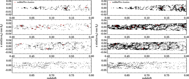
Figure 10. Cone diagrams for HectoMAP DR1: (left) galaxies from SDSS/BOSS and (right) HectoMAP. Red circles indicate redMaPPer clusters (Section 3.1).
Download figure:
Standard image High-resolution imageSutter et al. (2014) emphasize the importance of dense sampling for the definition of void sizes, shapes, and density profiles. Hwang et al. (2016) compare a volume-limited subsample of the HectoMAP data with the 300 mock surveys drawn from the Horizon Run 4 N-body simulation to show the efficacy of HectoMAP in defining the elements of the large-scale structure in the universe. The data and the models are in excellent agreement. The full HectoMAP sample will provide a test bed for void evolution for z ≲ 0.7.
HectoMAP has already provided a test (Sohn et al. 2018b) of the photometric RM cluster catalog (Rykoff et al. 2014, 2016) over the redshift range 0.08 < z < 0.6. About 90% of the RM systems in the HectoMAP footprint correspond to systems in the HectoMAP survey. This test included even low-richness RM systems. On average HectoMAP provides a spectroscopic redshift for ∼20 cluster members. At redshift z > 0.35, the HectoMAP spectroscopic richness does not correlate well with the RM richness, but the HectoMAP target selection could be an issue (Sohn et al. 2018b). We reconsider the RM systems in HectoMAP DR1 in Section 3.1 below.
2.5. Dn 4000
We compute the stellar population age-sensitive indicator Dn 4000. This spectral index is the flux ratio between two spectral windows (3850–3950 Å and 4000–4100 Å) near the 4000 Å break (Balogh et al. 1999). Fabricant et al. (2008) show that the typical error in Dn 4000 is 0.045 times the value of the index, and for spectra overlapping with the SDSS, agreement is excellent. We include a value of Dn 4000 for more than 99% of the objects in both the bright and faint red-selected subsamples of HectoMAP (Table 3). For 1% of objects, we could not measure Dn 4000 because the redshifts come from the NED.
Table 3. Completeness of Stellar Mass and Dn 4000 Measurements
| Subsample | Nspec |
 a | fM* b |
 c |
|---|---|---|---|---|
| All | 17313 | 99.0 | 99.9 | 64.3 |
| g − r > 1, r < 20.5 | 8117 | 99.3 | 99.9 | 78.3 |
| g − r > 1, 20.5 ≤ r < 21.3 | 4876 | 99.8 | 100.0 | 64.6 |
Notes.
a is the fraction of galaxies with Dn
4000 measurements.
b
fM* is the fraction of galaxies with stellar mass estimates.
c
 is the fraction of galaxies with Dn
4000 > 1.5 among the galaxies with spectroscopic redshifts.
Download table as: ASCIITypeset image
Panels (a) and (b) of Figure 11 show the redshift and absolute magnitude distributions for the entire HectoMAP DR1 sample (black), the bright red-selected sample (red hatched histogram), and the faint red-selected sample (blue). The faint sample includes mostly galaxies at z > 0.4 with a tail of intrinsically lower luminosity (lower stellar mass) objects toward lower redshift; these objects are evident in panel (d). The bright red-selected sample peaks around the z ∼ 0.3 with a significant extension of intrinsically luminous galaxies at z > 0.4. These fiducial distributions underlie the distributions of other derived physical properties in panels (c) and (d).
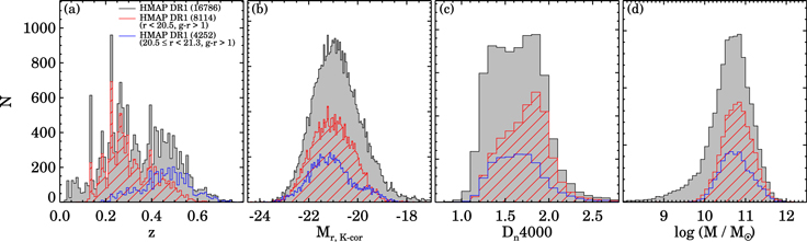
Figure 11. Distributions of HectoMAP DR1 galaxy properties: (a) redshift, (b) K-corrected absolute magnitude, (c) Dn 4000, (d) stellar mass. Black shaded histograms show all HectoMAP DR1 galaxies. Red hatched and blue open histograms display galaxies in the bright red subsample (r < 20.5 mag and (g − r)model,0 > 1.0) and in the faint red subsample (20.5 ≤ rpetro,0 (mag) < 21.3, (g − r)model,0 > 1.0, (r − i)model,0 > 0.5), respectively.
Download figure:
Standard image High-resolution imageFigure 11(c) shows the Dn 4000 distribution for all of the galaxies in HectoMAP DR1 (open histogram). The red hatched histogram shows the Dn 4000 distribution for the bright red-selected subsample with r < 20.5 and (g − r) > 1.0. The red color selection moves the Dn 4000 distribution for bright red-selected sample toward higher Dn 4000 as expected. The blue histogram shows the Dn 4000 for the faint red-selected sample. The peak shifts toward lower Dn 4000, an indication of the younger stellar age of the galaxies.
Table 3 lists the fraction of galaxies with Dn 4000 > 1.5 in each subsample. We use this cut as a proxy for identifying the quiescent population (e.g., Moresco et al. 2013; Damjanov et al. 2018). Because of the red selection, quiescent galaxies dominate HectoMAP DR1. For the bright sample, the fraction of Dn 4000 > 1.5 galaxies exceeds that for the fainter sample primarily as a result of the combination of the fixed observed color cuts and the lower median redshift of the subsample.
2.6. Stellar Mass
For consistency with previous MMT redshift surveys (e.g., Geller et al. 2014; Zahid et al. 2016), we calculate stellar masses based on SDSS ugriz model magnitudes corrected for foreground extinction. We fit the observed spectral energy distribution (SED) with the Le PHARE fitting code (Arnouts et al. 1999; Ilbert et al. 2006). We use the stellar population synthesis models of Bruzual & Charlot (2003), and we assume a universal Chabrier initial mass function (Chabrier 2003). We consider a suite of models with two metallicities and with exponentially declining star formation rates. The e-folding times for the star formation ranges from 0.1 to 30 Gyr. Model SEDs include various extinction levels and stellar population ages. We explore the internal extinction range E(B − V) = 0 − 0.6 based on the Calzetti et al. (2000) extinction law. The population age range is 0.01–13 Gyr. We normalize each SED to solar luminosity. The ratio between the observed and synthetic SED is the stellar mass. We take the median of the distribution of best-fit stellar masses as the estimate of the stellar mass for a particular object.
Figure 11(d) shows the stellar mass distribution for HectoMAP DR1. Figure 12 displays the stellar mass as a function of redshift for HectoMAP DR1 objects. The lower stellar mass objects at fixed redshift have lower Dn 4000. Essentially all of the galaxies in HectoMAP DR1 have a stellar mass estimate (Table 3); the few objects without stellar mass estimates have inconsistent photometry (particularly in the u band). The stellar mass distribution for the bright red-selected subsample (red hashed histogram) contains a relatively larger fraction of massive objects than the entire DR1 sample (black histogram). Bluer objects with lower stellar mass dominate the low stellar mass tail of the black histogram; for these objects HectoMAP is not complete. In contrast, the red hashed histogram represents a highly complete subsample (Table 1).
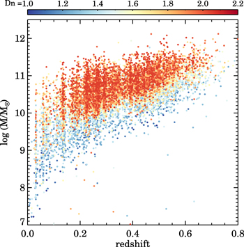
Figure 12. Stellar mass as a function of redshift for the HectoMAP DR1 objects, color coded by Dn 4000.
Download figure:
Standard image High-resolution image3. Two Examples of HectoMAP Applications
The HectoMAP survey has broad applications including computation of statistical measures of large-scale structure and comparison of the large-scale matter distribution as traced by galaxies and by weak lensing. We plan to address these and other issues in future work.
Here we highlight two straightforward applications of HectoMAP: details of photometrically identified RM clusters of galaxies as revealed by spectroscopy and a test of HSC photometric redshifts at bright magnitudes. The dense sampling of HectoMAP is designed for examining the properties and evolution of clusters of galaxies at redshifts from 0.2 to 0.7. Section 3.1 uses the current larger HectoMAP data set to enhance the results of Sohn et al. (2018b) and Sohn et al. (2018a). Section 3.2 tests the power of HectoMAP as a probe of the accuracy of HSC SSP photometric redshifts. These applications highlight both the strengths (e.g., density, depth, and completeness) and limitations (e.g., color selection) of the HectoMAP survey.
3.1. redMaPPer Clusters
One of the central goals of HectoMAP is construction of a spectroscopy-based catalog for systems with M ≳ 1014 M⊙ and redshift z ≤ 0.5. Ultimately HectoMAP will be the basis for a cluster catalog based on a robust combination of photometric, X-ray, weak lensing, and spectroscopic methods. In fact, application of a friends-of-friends algorithm (e.g., Huchra & Geller 1982; Ramella et al. 2002; Robotham et al. 2011; Tempel et al. 2016) applied to an earlier version of the entire HectoMAP catalog provided 166 friends-of-friends systems for comparison with existing X-ray catalogs (Sohn et al. 2018a).
Sohn et al. (2018b) use HectoMAP to test the RM catalog (Rykoff et al. 2014, 2016), a prototype for photometric cluster identification and cluster membership probabilities. In that study, the median number of spectroscopic HectoMAP members of the 104 RM clusters is ∼20. Even at the lowest RM richness, the fraction of real systems (purity) of the RM catalog is impressively high, ∼90%. Figure 10 shows the 23 RM clusters in HectoMAP DR1 superimposed on the redshift survey cone diagram. The correspondence between the two catalogs is striking. In many cases the finger (elongation) in redshift space that corresponds to the cluster is apparent.
At the time of the Sohn et al. (2018b) analysis, the HectoMAP selection included a restriction on (r − i) for galaxies with r < 20.5. This cut led to a systematic undersampling of clusters at redshift z < 0.2. Removal of this cut improved the sampling as expected; the enhanced observations add 114 (∼9%) redshifts for RM cluster member candidates with Pmem > 0 (Pmem is the radial and luminosity weighted RM membership probability; Rykoff et al. 2014) in the HectoMAP DR1 region along with 25 new spectroscopic members not identified by RM.
The (r − i) selection remains an issue for one RM cluster candidate, HMRM13503 (Table 4). The typical spectroscopic survey completeness for RM member candidates with (r − i) < 0.5 and Pmem > 0.5 is ∼70%. However, the completeness for HMRM13503 is only ∼21% because HMRM13503 is near the survey boundary. We have spectroscopic redshifts for only two member candidates with Pmem > 0.5. The low survey completeness prevents derivation of a spectroscopic redshift for this cluster candidate. Thus, we use the photometric redshift of the system from the RM catalog. We include HMRM13503 in Figures 13 and 14, but we limit further comments to the 22 more uniformly sampled systems.
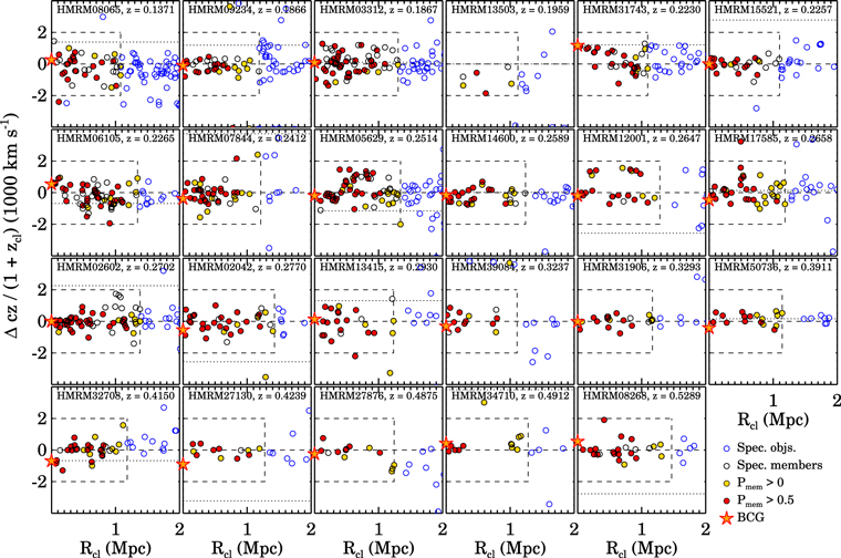
Figure 13. R–v diagrams for redMaPPer cluster candidates in HectoMAP DR1. Red and yellow filled circles indicate member candidates with Pmem ≥ 0.5 and 0.5 > Pmem > 0.0, respectively, identified by redMaPPer. Blue open circles show additional galaxies with spectroscopy at large projected radius. The orange star indicates the central galaxy identified by redMaPPer. The dashed box indicates the limits of member selection for the DR1-redMaPPer comparison in Table 4. Open circles inside this box indicate spectroscopic members identified by HectoMAP. The dashed horizontal line shows the mean spectroscopic redshift of the system, and the dotted line shows the photometric redshift determined by redMaPPer. Note that the redMaPPer photometric redshift may lie outside the display box (see Table 4).
Download figure:
Standard image High-resolution image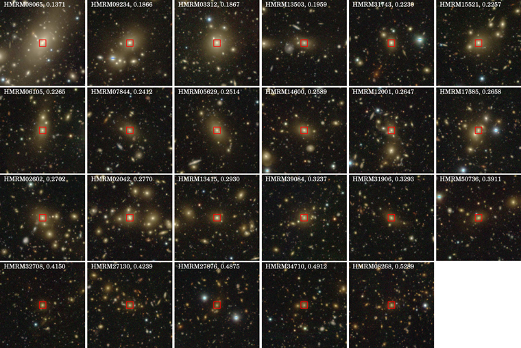
Figure 14. Subaru/HSC images of the 23 redMaPPer clusters in HectoMAP DR1. Each image shows a  field. A red square marks the central galaxy in each image. The labels indicate the redMaPPer ID and the redshift of the system. The color channels R, G, and B of the thumbnails are HSC-i, HSC-r, and HSC-g, respectively.
Download figure:
Standard image High-resolution imageTable 4. redMaPPer Clusters in HectoMAP DR1
| ID | R.A. | Decl. | Nmem>0 a | Nmem>0.5 b | Nspec,mem c | λd | zphot | zspec e |
|---|---|---|---|---|---|---|---|---|
| HMRM08065 | 245.362203 | 42.761316 | 40/28/24 | 25/19/17 | 39 | 26.55 ± 2.39 | 0.1424 ± 0.0045 | 0.1371 |
| HMRM09234 | 246.598995 | 42.889029 | 52/49/24 | 24/24/16 | 33 | 24.92 ± 2.46 | 0.1913 ± 0.0053 | 0.1866 |
| HMRM03312 | 246.677190 | 42.669934 | 56/49/43 | 45/42/40 | 63 | 41.28 ± 3.09 | 0.1871 ± 0.0050 | 0.1867 |
| HMRM13503 | 244.826793 | 42.769710 | 38/13/ 4 | 24/ 5/ 2 | 6 | 23.37 ± 2.20 | 0.1959 ± 0.0060 | 0.1959 |
| HMRM31743 | 248.862917 | 43.163936 | 35/33/26 | 24/23/21 | 33 | 20.17 ± 2.30 | 0.2279 ± 0.0080 | 0.2230 |
| HMRM15521 | 246.874333 | 42.896084 | 37/31/18 | 25/19/16 | 26 | 24.46 ± 2.64 | 0.2371 ± 0.0085 | 0.2257 |
| HMRM06105 | 248.785849 | 42.800077 | 72/52/39 | 43/32/29 | 60 | 40.45 ± 3.45 | 0.2237 ± 0.0068 | 0.2265 |
| HMRM07844 | 245.321364 | 42.954352 | 58/50/34 | 32/31/25 | 40 | 31.25 ± 2.64 | 0.2566 ± 0.0097 | 0.2412 |
| HMRM05629 | 243.443971 | 43.268378 | 73/57/44 | 40/35/31 | 57 | 38.78 ± 3.10 | 0.2466 ± 0.0083 | 0.2514 |
| HMRM14600 | 242.339068 | 42.919114 | 58/43/24 | 28/22/17 | 28 | 28.29 ± 2.90 | 0.2590 ± 0.0100 | 0.2589 |
| HMRM12001 | 246.508451 | 43.704142 | 70/43/22 | 34/24/17 | 24 | 32.16 ± 3.27 | 0.2539 ± 0.0094 | 0.2647 |
| HMRM17585 | 245.464063 | 43.093565 | 56/44/34 | 26/24/19 | 36 | 27.05 ± 2.86 | 0.2664 ± 0.0103 | 0.2658 |
| HMRM02602 | 248.482328 | 43.091167 | 81/62/47 | 53/46/39 | 59 | 49.48 ± 3.49 | 0.2798 ± 0.0106 | 0.2702 |
| HMRM02042 | 247.063222 | 43.813437 | 98/66/30 | 52/41/24 | 34 | 49.29 ± 3.37 | 0.2660 ± 0.0093 | 0.2770 |
| HMRM13415 | 244.422275 | 42.539315 | 54/29/19 | 32/21/16 | 22 | 30.56 ± 2.86 | 0.2987 ± 0.0125 | 0.2930 |
| HMRM39084 | 248.935265 | 42.628005 | 64/27/12 | 22/11/10 | 14 | 23.19 ± 2.83 | 0.3769 ± 0.0194 | 0.3237 |
| HMRM31906 | 248.205718 | 43.390310 | 62/36/16 | 24/17/11 | 20 | 24.05 ± 2.81 | 0.3532 ± 0.0184 | 0.3293 |
| HMRM50736 | 247.060881 | 43.217691 | 57/26/18 | 20/12/11 | 18 | 24.58 ± 3.45 | 0.3919 ± 0.0153 | 0.3911 |
| HMRM32708 | 247.752305 | 43.033666 | 50/34/28 | 21/20/17 | 32 | 23.37 ± 3.45 | 0.4118 ± 0.0147 | 0.4150 |
| HMRM27130 | 249.234246 | 43.923393 | 52/23/12 | 26/10/ 8 | 13 | 27.46 ± 3.38 | 0.4086 ± 0.0155 | 0.4239 |
| HMRM27876 | 243.171435 | 43.416313 | 46/15/12 | 24/ 9/ 8 | 13 | 44.21 ± 8.56 | 0.5200 ± 0.0168 | 0.4875 |
| HMRM34710 | 243.046178 | 43.658707 | 48/22/12 | 17/ 8/ 6 | 12 | 38.05 ± 7.60 | 0.5102 ± 0.0155 | 0.4912 |
| HMRM08268 | 247.456116 | 43.839720 | 69/28/20 | 38/19/16 | 24 | 68.94 ± 10.86 | 0.5147 ± 0.0142 | 0.5289 |
Notes.
a Number of member candidates/number of candidates with spectroscopy/spectroscopically identified members with Pmem > 0. b Number of member candidates/number of candidates with spectroscopy/spectroscopically identified members with Pmem > 0.5. c Number of spectroscopically identified members within ∣Δcz/(1 + zcl)∣ < 2000 km s−1. d Richness from the redMaPPer catalog. e HectoMAP spectroscopic redshift of the system.Download table as: ASCIITypeset image
Figure 13 shows phase space diagrams for all of the HectoMAP DR1 RM cluster candidates (ordered by redshift) with richness larger than 20. To derive the mean spectroscopic redshift for a system, we first select probable cluster members with Pmem > 0.5 that have spectroscopic redshifts. We compute the median redshift of these probable members and iterate by removing 3σ outliers. The median redshift of the remaining spectroscopically confirmed RM members is the cluster spectroscopic redshift.
In Figure 13, red and yellow filled circles show member candidates identified by the RM algorithm: red circles indicate an RM membership probability Pmem > 0.5, and yellow circles indicate 0.5 > Pmem > 0, respectively. In general, the RM candidate members with Pmem > 0.5 are closer to the cluster center (see also Sohn et al. 2018b). The photometric redshift from the RM catalog indicated by the dotted line is often offset from the spectroscopic redshift. The mean (median) offset is 1300 km s−1 (1200 km s−1), and the dispersion in the offset is 3500 km s−1. This difference and scatter result from error in the photometric redshift (∼3000 km s−1) and from the impact of foreground/background structures unresolved by RM.
The membership identification window finds members within a projected separation RRM and a rest-frame radial velocity difference Δ = ∣(c(zgalaxy − zcl)/(1 + zcl)∣ < 2000 km s−1, where RRM is a projected clustercentric radius, zgalaxy is the spectroscopic redshift of the potential cluster member, and zcl is the spectroscopically determined cluster central redshift. We set the RRM limit to match the maximum RRM of the RM candidate members in each cluster (Rykoff et al. 2014). This boundary tends to be larger for richer systems. We choose the relative rest-frame velocity limit by assessing the maximum range of spectroscopically identified members in known massive clusters (e.g., HeCS, Rines et al. 2013, 2016, 2018). The resulting spectroscopic membership is insensitive to variations in Δ over the range 1500–2500 km s−1. Column 11 of Table 2 indicates spectroscopically determined RM cluster membership.
The RM candidate member list includes galaxies with r < 22 mag. Thus HectoMAP with its limit of r = 21.3 mag does not include the apparently faintest candidates. HectoMAP also does not generally include objects bluer than (r − i) = 0.5 for r > 20.5 mag. Table 4 shows that the fractional completeness of the HectoMAP census of cluster member candidates generally decreases with the cluster redshift; HMRM13503 is an exception as a result of observational issues as discussed above. The number of cluster members identified by spectroscopy generally increases with the RM richness at a given redshift. The number of spectroscopically identified members ranges from 50 to 60 for richer systems (RM richness λ ≳ 40) at low redshift to 12–24 for systems of similar richness at redshift z ≳ 0.3. At z ≳ 0.3 the HectoMAP sampling is often limited because most of the candidate members are fainter than the HectoMAP apparent magnitude limit. As expected, throughout the sample, a higher fraction of RM Pmem > 0.5 candidates are confirmed by spectroscopy.
In a few cases apparently rich RM systems are inflated by structure superposed along the line of sight (e.g., HMRM12001, where only ∼50% of the RM Pmem > 0 candidates are spectroscopic members). At lower redshift, the broader color selection for galaxies with r < 20.5 in HectoMAP yields a larger sample of cluster members identified by spectroscopy but not included as RM candidate members. A median 32 RM members are confirmed by spectroscopy in the 22 RM clusters (column 6 of Table 4).
The RM central galaxies are obvious in the Subaru HSC images (Figure 14). Each HSC image shows a  region centered on the RM central. Four clusters, 31743, 06105, 07844, and 08268, contain a spectroscopic member brighter than the RM central in the SDSS r band. The fraction of RM clusters with a galaxy brighter than the central is 18%, consistent with the estimates by Rykoff et al. (2016) and Sohn et al. (2018b). In three of these systems, the brightest galaxy is significantly offset (∼370 kpc) from the RM center and the density of cluster members around the RM central is greater than that around the brighter member. For the cluster HMRM08268, the brightest galaxy is possibly a better choice for the cluster center.
Figure 15 displays the HSC image of HMRM08268 (at z = 0.528). A red square marks the RM central, and a red circle indicates the brightest spectroscopic member. Surprisingly, there are apparent strong lensing arcs associated with both the RM central and the brightest member. The projected separation between the two bright galaxies is ∼560 kpc, and their relative rest-frame velocity is ∼675 km s−1. In this system, clustering around the brightest member is more impressive than it is around the RM central. HMRM08268 is the subject of an intensive spectroscopic campaign with the MMT and Keck (J. Sohn et al. 2021, in preparation); it is a candidate merging cluster.
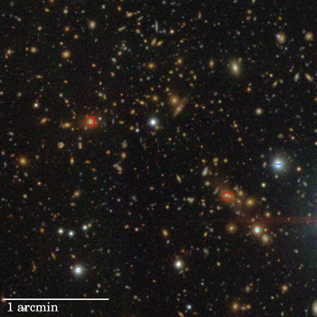
Figure 15. Subaru/HSC image of HMRM08268 (z = 0.528). The red square indicates the RM central galaxy, and the red circle indicates the brightest member. Both the RM central and the brightest galaxy are associated with several strong lensing arc candidates.
Download figure:
Standard image High-resolution imageThe census of RM candidate systems in the HectoMAP DR1 confirms that these richness λ > 20 are bona fide clusters of galaxies. The spectroscopy provides important refinements of system membership by eliminating foreground/background contamination and by identifying additional members not included in the RM member candidate lists (Table 4). The survey also underscores the reliability of the RM central identification as an excellent proxy for the Brightest Cluster Galaxy; the most striking departure, HMRM08268, is an interesting case that highlights the impact of spectroscopy in a comprehensive survey.
The RM systems are one element of the multitechnique cluster catalog enabled by HectoMAP. We plan to combine a redshift-based catalog, X-ray detections from e-ROSITA (Finoguenov et al. 2019; Sohn et al. 2019), and weak lensing detections from HSC data to construct this catalog of clusters with z ≲ 0.55. The HSC imaging also makes a platform for identifying a set of strong lensing system candidates like HMRM08268.
Stacked sets of clusters from this HectoMAP cluster catalog combined with lower-redshift systems sampled well to large radius (e.g., Rines & Diaferio 2006; Rines et al. 2013, 2016) enable investigations of cluster growth. The redshift range encompasssed by HectoMAP is interesting because simulations and analytic models show that z = 0 clusters with masses of 1014-15 M⊙ accreted half of their mass at an approximately constant rate between z ∼ 0.5 and the current epoch (van den Bosch et al. 2014; Correa et al. 2015; Pizzardo et al. 2021). Pizzardo et al. (2021) develop a technique for direct measurement of the cluster accretion rate as a function of cluster mass and epoch. The small subset explored here predicts the rough number of spectroscopic members in stacked systems, the platform for a first direct dynamical test of the accretion history models in the HectoMAP redshift range.
3.2. Test of HSC Photometric Redshifts
Increasingly extensive photometric surveys make use of photometric redshifts (hereafter, zphots) imperative for studying galaxy evolution and for limiting the cosmological parameters. Larger and larger surveys with well-calibrated photometry in five or more bands have prompted more and more sophisticated development of zphot estimators. Template fitting along with more recent applications of machine learning provide platforms for analyzing the challenging current and future data sets. Tanaka et al. (2018) also develop a hybrid technique they call FrankenZ that combines the strengths of template fitting and machine learning.
Tanaka et al. (2018) train a variety of zphot estimators with a large, careful compilation of 170,000 spectroscopic redshifts (zspec) extending to z ∼ 4. They then provide a variety of performance tests and demonstrate the efficacy of zphot over the redshift range 0.2 < z < 1.5. Here we complement their investigation with HectoMAP DR1. The entire HectoMAP survey will provide a uniform sample of more than 110k redshifts for detailed tests of zphot for z ≲ 0.7.
We compare the HectoMAP DR1 zspec with HSC zphot. We use zphots from the public HSC SSP DR2 catalog. The catalog provides only two of the zphot estimators explored by Tanaka et al. (2018): DeMP and Mizuki, a template-fitting code (Tanaka 2015). Because of its better performance (Tanaka et al. 2018), we examine ∼110,000 zphot computed with the DeMP code (Hsieh & Yee 2014) for objects brighter than r = 22 mag in the HectoMAP DR1 region. The DeMP code fits each input galaxy based on a subset of the training set with photometry and colors closest to the target object. Tanaka et al. (2018) use their dense training set to apply this regional polynomial fitting to the HSC data.
Among the HSC SSP public DR2 objects, 17,040 (∼10% of the number of galaxies in the Tanaka et al. (2018) spectroscopic training sample) have a HectoMAP zspec. The dense, relatively bright, red-selected HectoMAP sample complements the generally deeper data sets used by Tanaka et al. (2018). HectoMAP provides a test bed largely independent of the Tanaka et al. (2018) training sets, thus complementing their results.
Figure 16(a) shows the DeMP zphot as a function of the HectoMAP zspec. The two redshifts generally follow a one-to-one relation, but the scatter is large. Circles mark the median of the photo-z distribution in each zspec bin. There are small systematic shifts as a function of redshift. Extensions along the zphot direction occur where zphot differs substantially from zspec.
Figure 16(b) shows the difference between the photometric and spectroscopic redshifts as a function of spectroscopic redshift. The red symbols show the median redshift difference. In the zspec interval 0.2–0.4, the median zphot exceeds zspec. Overall, the median redshift difference is 0.004 ± 0.047. This typical redshift difference (∼1100 km s−1) corresponds to the line-of-sight velocity dispersion of massive galaxy clusters.
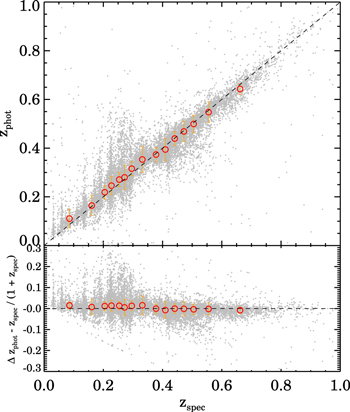
Figure 16. (a) Comparison between spectroscopic redshifts and DeMP zphots from the HSC catalog in HectoMAP DR1. Red circles show the median of the distribution in each spectroscopic redshift bin. (b) Difference between zspec and zphot as a function of zspec.
Download figure:
Standard image High-resolution imageThe accuracy of the zphot measurements is a strong function of apparent magnitude. Figure 17 shows the difference between photometric and spectroscopic redshifts as a function of r-band magnitude for galaxies in the spectroscopic redshift range 0.2 < zspec < 0.3. The red squares indicate the median difference. The redshift difference increases at fainter magnitude (r > 20 mag). Furthermore, the number of outliers (∣Δz∣ > 0.15) is also high at r > 20. A similar test at higher redshift requires a survey to a fainter magnitude limit.
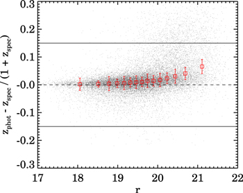
Figure 17. Difference between photometric and spectroscopic redshifts as a function of rpetro,0 for HectoMAP DR1 galaxies with 0.2 < zspec < 0.3 (gray points). The red symbols show the median and 1σ standard deviation.
Download figure:
Standard image High-resolution imageFigure 18 is a visual demonstration of the impact of zphot on the large-scale structure. For ease of direct comparison, the left-hand panel of the figure shows the cone diagrams of Figure 10. The points indicate individual galaxies, and the red dots show the positions of RM clusters in redshift space. The right-hand panel shows the cone diagrams based on DeMP zphot. The error in a typical DeMP zphot is 0.05 ± 0.12 or, equivalently, ∼15,000 km s−1. Overall large-scale density gradients are approximately preserved, but the filaments, walls, and voids characteristic of the large-scale structure of the universe become invisible.
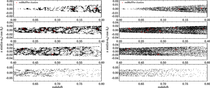
Figure 18. Cone diagrams for HectoMAP DR1 based on spectroscopic redshifts (left) and photometric redshifts (right).
Download figure:
Standard image High-resolution imageTanaka et al. (2018) use a variety of metrics to test their zphot algorithms (see also Pasquet et al. 2019). For comparison with their analysis, we compute three metrics for the HectoMAP DR1 sample: the bias, dispersion, and loss rate.
The bias measures the systematic offset, if any, between the photometric and spectroscopic redshifts. As in Tanaka et al. (2018) we compute

Figure 19 shows the median value of this offset as a function of i, zphot, and zspec (red points). Lines in the left-hand panel of Figure 19 show the analogous results of Tanaka et al. (2018) (their Table 2). For this measure, the agreement between the HectoMAP DR1 test and the Tanaka et al. (2018) test bed is remarkable. There is essentially no dependence of the bias on either the apparent magnitude or the photo-z (central panel of Figure 19). In contrast with Tanaka et al. (2018), we also plot the metrics as a function of zspec (right-hand panel of Figure 19). Over the redshift range we sample, the bias changes systematically with zspec; at lower redshifts the photometric estimate overestimates the redshift, and at the highest redshift, the zphot is an underestimate. This behavior is also evident in Figure 16.
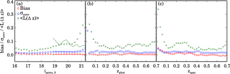
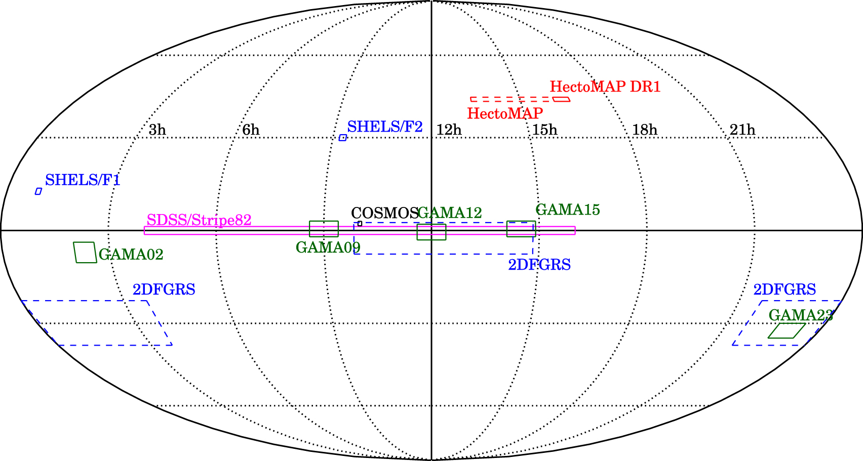
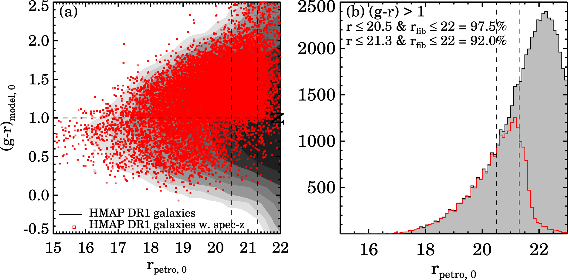
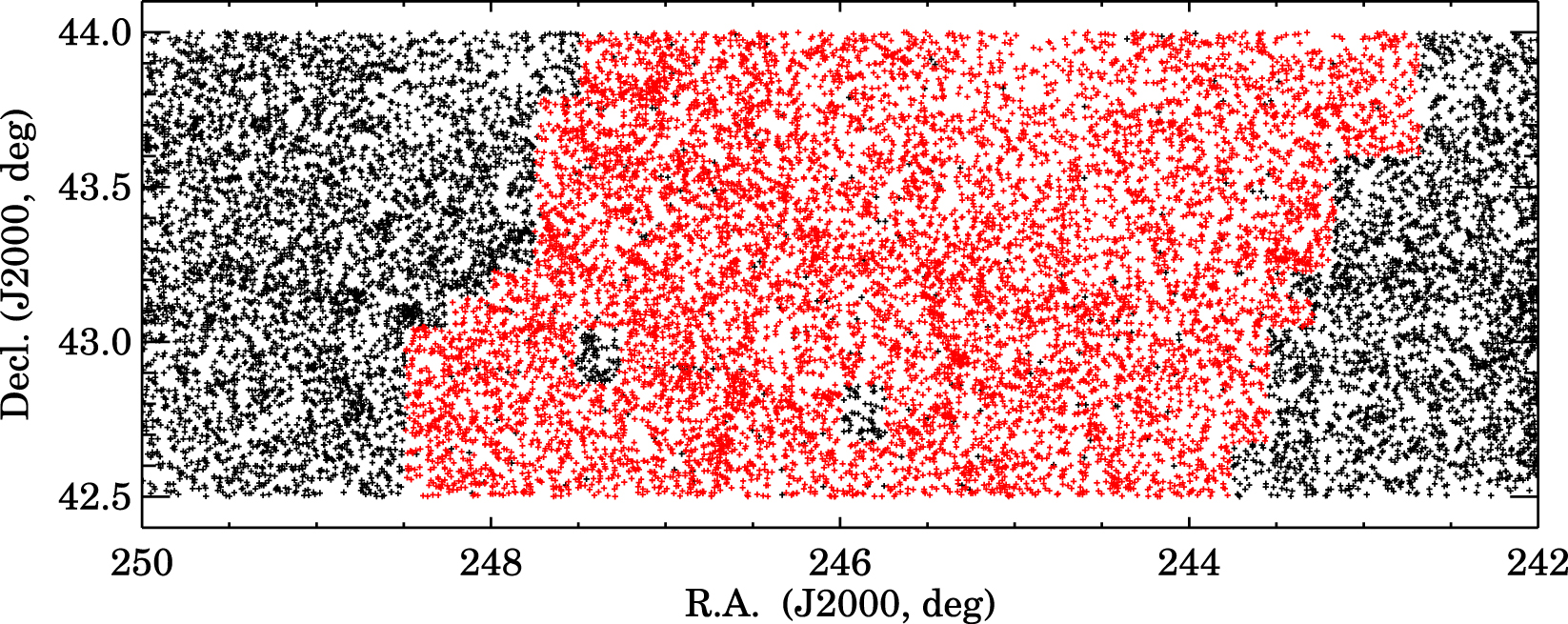
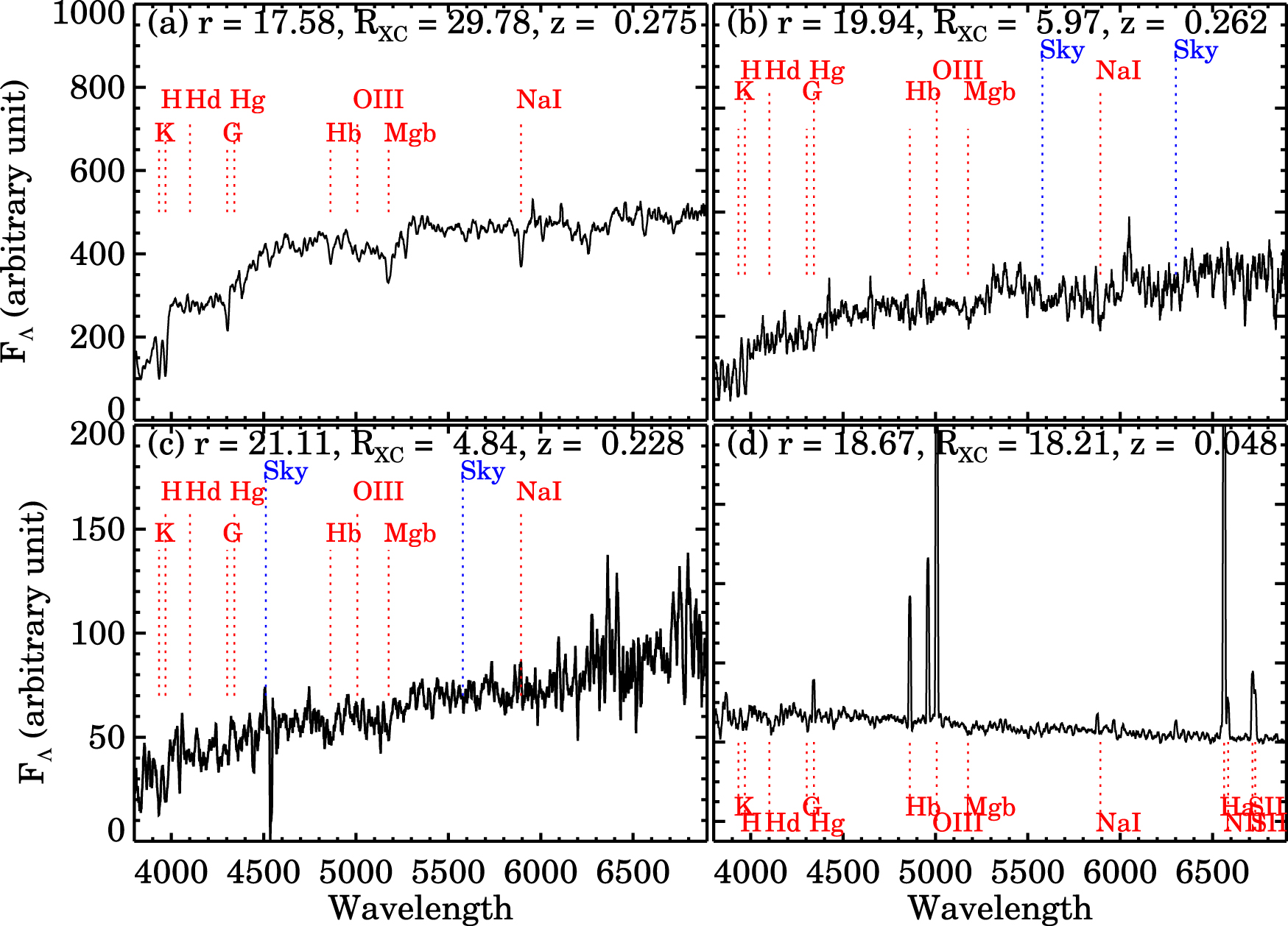
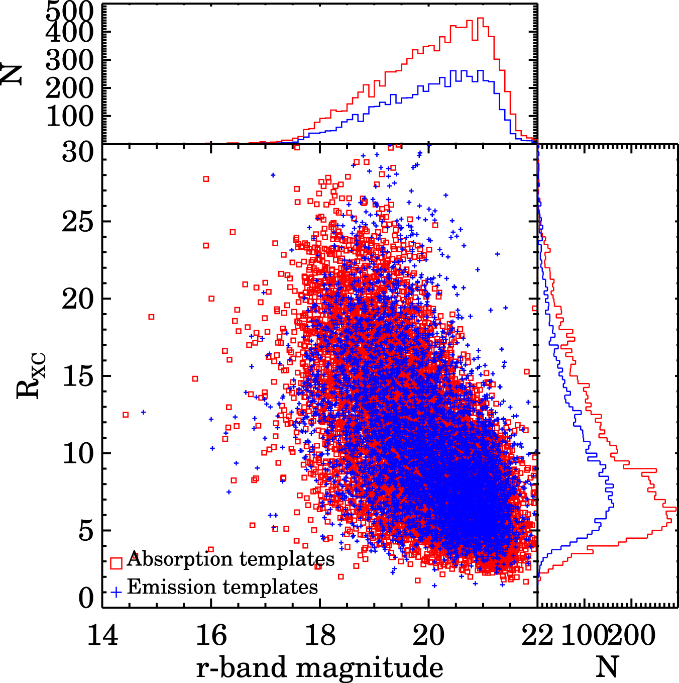
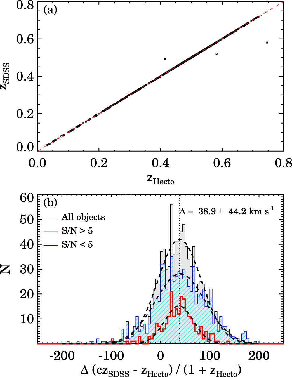
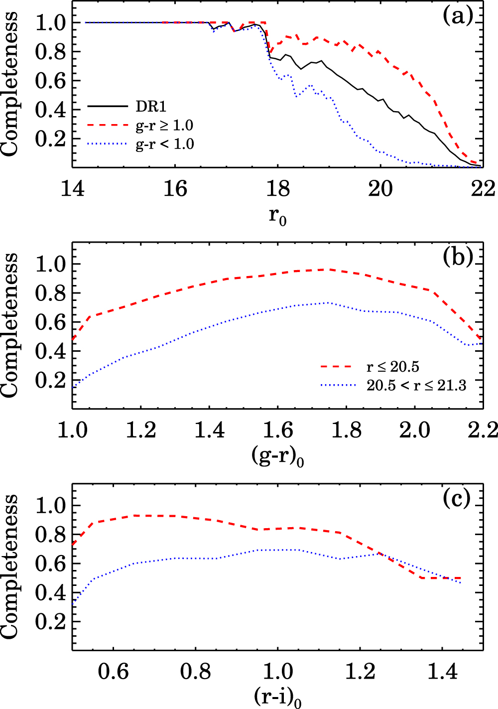
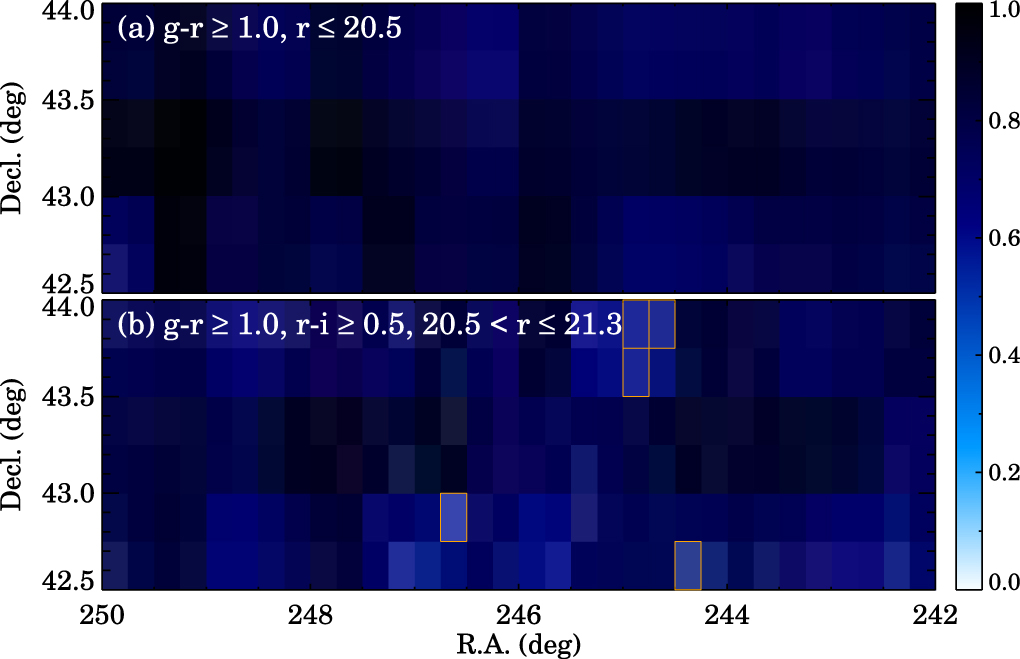
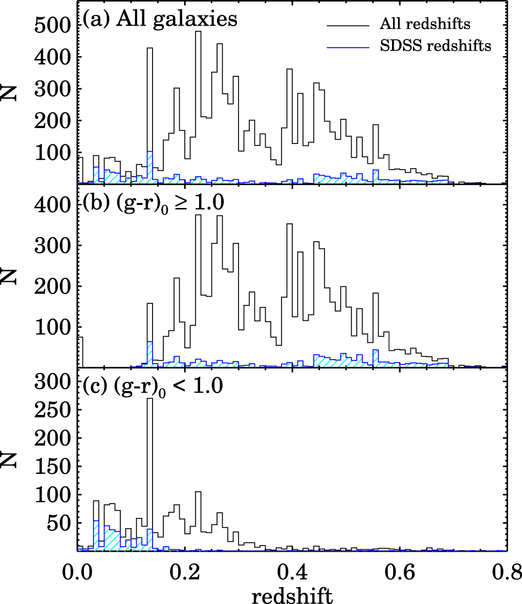
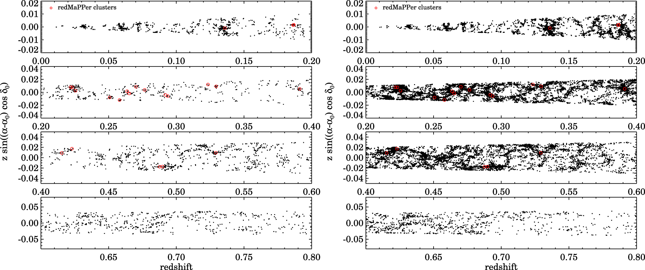
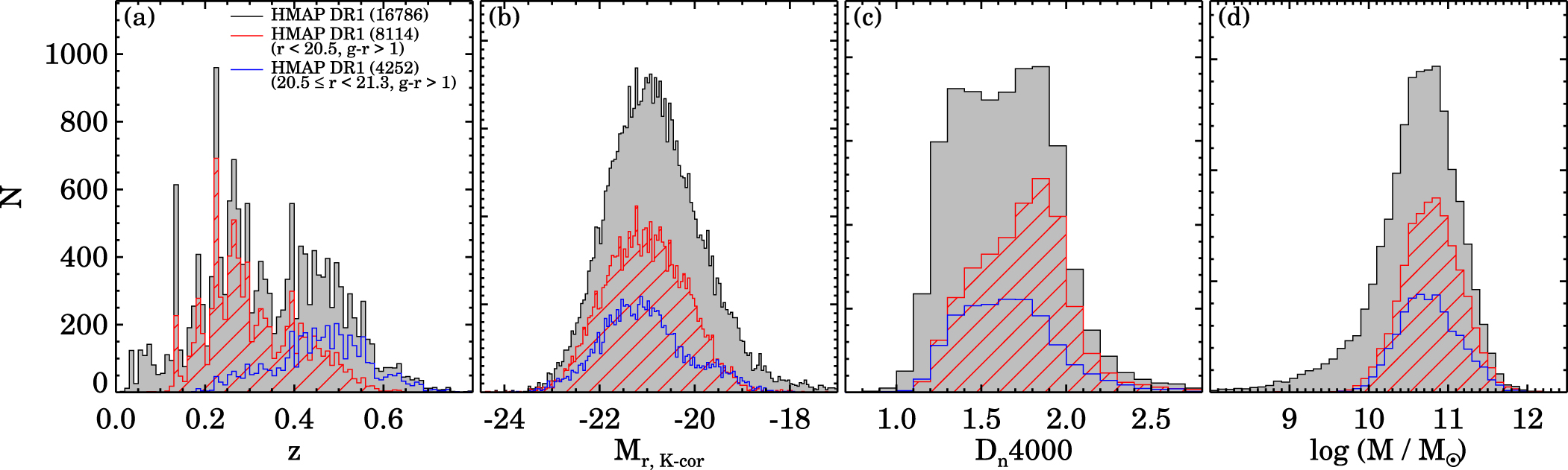
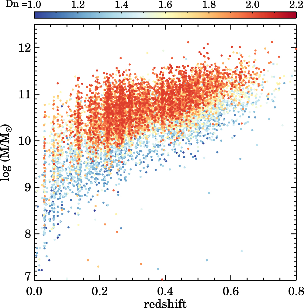
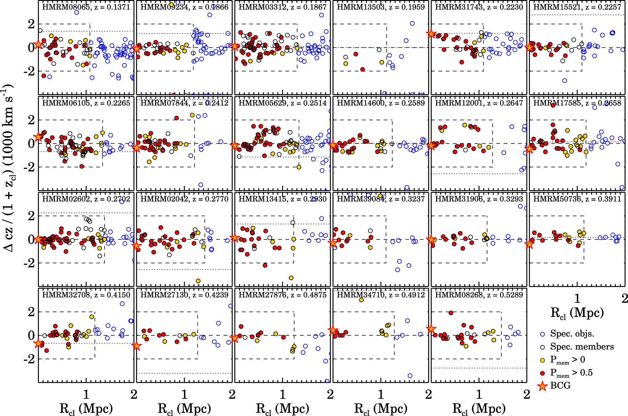
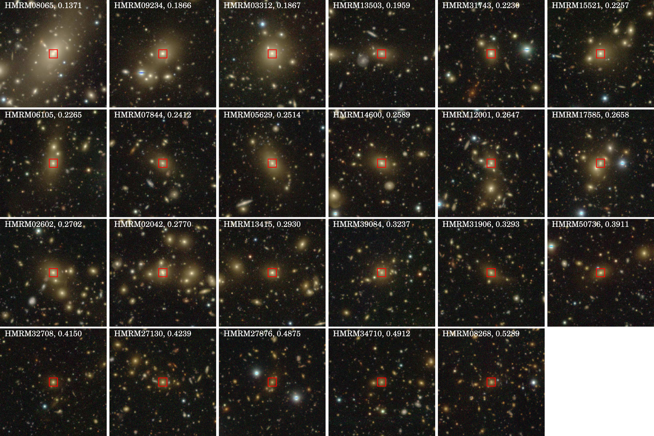
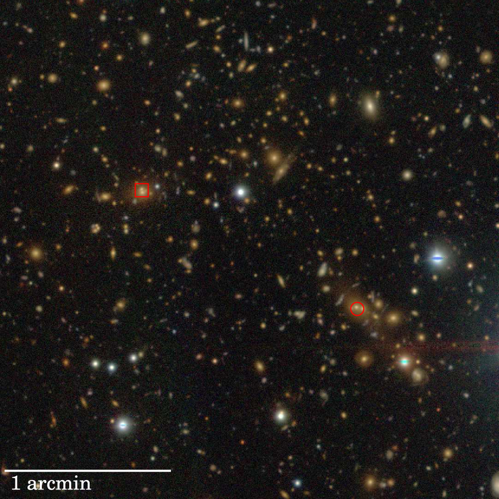
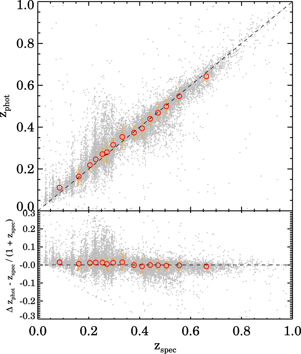
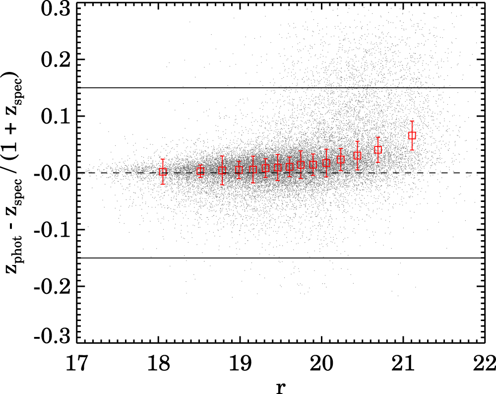
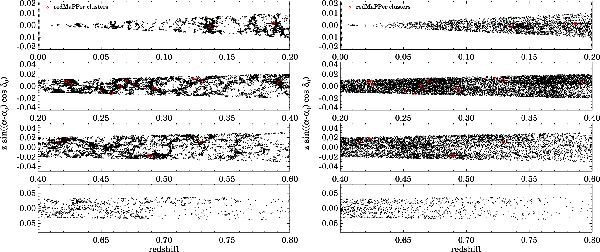
Figure 19. Left: bias (red points), σconv (blue points), and < L(Δz) > (green points) of zphot,DeMP as a function of SDSS i-band magnitude. The correspondingly colored lines show comparable results from Tanaka et al. (2018). Middle: same as the left panel but as a function of zphot. Right: same as the left panel but as a function of zspec.
Download figure:
Standard image High-resolution image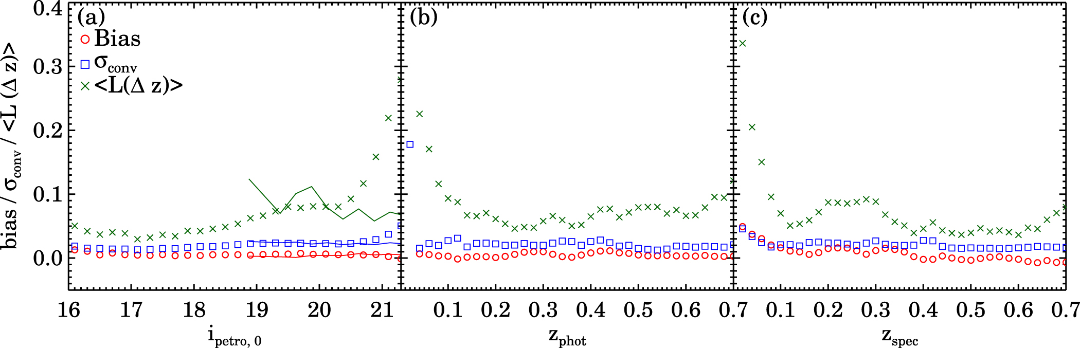
Next we compute the conventional dispersion

The MAD (Δz) is the median absolute Δz. Blue points in Figure 19 show the result. In the overlapping apparent magnitude range, the agreement with Tanaka et al. (2018) is excellent. The dispersion increases slightly for fainter apparent magnitudes as expected. The large dispersion at low spectroscopic redshift in the right-hand panel may result from the inclusion of more blue emission line objects at this redshift. At larger redshift, the HectoMAP DR1 test sample is dominated by absorption line objects as a result of the red selection.
Tanaka et al. (2018) develop a metric they call the loss function. This metric has the advantage of combining traditional metrics in a single function. The loss function is a continuous version of the outlier fraction that incorporates the impact of both the bias and dispersion. The expression for the loss function is

where Tanaka et al. (2018) adopt γ = 0.15 to reflect the standard limit Δz = 0.15 in the calculation of the outlier fraction.
Figure 19 shows the loss function for HectoMAP DR1 (green points) compared with the Tanaka et al. (2018) result (green line). For i-band magnitudes between 19 and 20, the results agree. At fainter magnitudes the loss function for HectoMAP exceeds the Tanaka et al. (2018) result. This difference is driven primarily by faint galaxies with spectroscopic redshifts in the range 0.2 < zspec < 0.3 (Figure 17). These galaxies have relatively low absolute luminosities, and some have low surface brightness.
The dependence of the loss function on photometric and spectroscopic redshift (center and right-hand panels of Figure 19) provides further insight into the subtleties of the relative behavior of the two measures. The loss function increases at zphot < 0.1. It rises slowly from zphot = 0.2 to zphot = 0.7, reflecting the large scatter visible in Figures 16 and 17. The scatter around the one-to-one correspondence between photometric and spectroscopic redshifts in Figure 16 is most pronounced in the redshift range 0.2 < zspec < 0.3. In the central panel of Figure 19 this scatter spreads the data over a wide range of zphot; in the right-hand panel where we display the dependence of the loss function of zspec, there is an obvious positive bump in the loss function confined to this range. The cleaner dependence of the loss function on spectroscopic redshift highlights the impact of the larger photo-z scatter and bias for faint objects in a relatively narrow redshift range (Figure 17).
Exploration of the HSC SSP zphot based on HectoMAP DR1 shows both the power and subtle limitations of the zphot. The HectoMAP analysis confirms and amplifies the results of Tanaka et al. (2018) for bright magnitudes and low redshifts. Comparison of spectroscopic and photometric redshifts as a function of spectroscopic redshift reveals a systematic bias that is a function of redshift; this bias does not appear either as a function of apparent magnitude or as a function of photometric redshift.
Investigation of other metrics, particularly the loss function, as a function of zspec shows that at least for red objects, the zphot perform well down to a redshift z = 0.15, in slight contrast to the z = 0.2 limit stated by Tanaka et al. (2018). The HectoMAP study complements Tanaka et al. (2018) by highlighting the impact of the increased bias and scatter of zphot for faint objects in a fixed spectroscopic redshift range. The full HectoMAP sample will enable this kind of detailed investigation over the redshift range 0.1–0.7.
4. Conclusion
HectoMAP is a dense red-selected redshift survey covering 54.64 deg2 to a limiting r = 21.3 mag in a narrow strip across the northern sky. The complete survey will include ∼110,000 redshifts. The first data release (HectoMAP DR1) covers 8.7 deg2. HectoMAP DR1 includes 17,313 galaxy redshifts along with stellar mass and Dn 4000 for nearly all of the galaxies. Among these galaxies, we acquired 14,767 redshifts with the Hectospec wide-field fiber instrument on the MMT.
The HSC SSP survey (Aihara et al. 2018) covers the entire HectoMAP region; HectoMAP DR1 encompasses the smaller area HSC SSP DR1 region. The combination of deep photometry and dense spectroscopy enables investigations that combine both strong and weak lensing with spectroscopy. The excellent seeing over large portions of the HSC SSP data also enables detailed investigations of the size evolution of the quiescent galaxy population.
We outline the quality and completeness of the HectoMAP DR1 data with an eye toward demonstrating its applications to problems in cosmology and large-scale structure. We emphasize the power of a dense survey in the study of the definition and evolution of voids and massive clusters over the redshift range 0.2–0.7.
As a demonstration of the applicability of HectoMAP to astrophysical and technical issues in large-scale structure we revisit the properties of RM clusters. The typical number of spectroscopic members of the 22 uniformly surveyed clusters is ∼31. The HectoMAP observations combined with the HSC SSP photometry highlight a fascinating merging system, HMRM08268 at z = 0.528. This system contains two luminous galaxies associated with strong lensing arcs. HMRM08268 is already the subject of a Keck telescope campaign.
We also highlight the insights HectoMAP provides on HSC SSP photometric redshifts. Dense coverage of the redshift range uncovers a subtle systematic bias in the median photometric redshift as a function of spectroscopic redshift. The HectoMAP data also show that in a fixed spectroscopic redshift range, 0.2–0.3, both the bias and the scatter in photometric relative to spectroscopic redshifts increase significantly for fainter objects. The full HectoMAP survey will provide similarly detailed tests for redshifts from 0.2 to 0.7.
HectoMAP currently fills a niche between large-volume surveys at lower redshift and surveys that reach to much greater redshift. Over the next few years a remarkable array of multiobject spectrographs on large facilities will provide dense surveys with much larger areal coverage in the HectoMAP range and beyond. HectoMAP enables initial explorations of many astrophysical issues that can inform the design of these future surveys.
We thank Perry Berlind and Michael Calkins for operating Hectospec. We also thank Susan Tokarz and Jaehyon Rhee for their important contributions to the data reduction. We thank Antonaldo Diaferio, Ken Rines, and Scott Kenyon for discussions that clarified the paper. This paper uses data products produced by the OIR Telescope Data Center, supported by the Smithsonian Astrophysical Observatory. J.S. gratefully acknowledges the support of a CfA Fellowship. The Smithsonian Institution supported the research of M.J.G., D.F., and S.M.M. This research has made use of NASA's Astrophysics Data System Bibliographic Services.
Funding for the SDSS-IV has been provided by the Alfred P. Sloan Foundation, the U.S. Department of Energy Office of Science, and the Participating Institutions. SDSS-IV acknowledges support and resources from the Center for High Performance Computing at the University of Utah. The SDSS website is www.sdss.org. SDSS-IV is managed by the Astrophysical Research Consortium for the Participating Institutions of the SDSS Collaboration including the Brazilian Participation Group, the Carnegie Institution for Science, Carnegie Mellon University, Center for Astrophysics ∣ Harvard and Smithsonian, the Chilean Participation Group, the French Participation Group, Instituto de Astrofísica de Canarias, Johns Hopkins University, Kavli Institute for the Physics and Mathematics of the Universe (IPMU)/University of Tokyo, the Korean Participation Group, Lawrence Berkeley National Laboratory, Leibniz Institut für Astrophysik Potsdam (AIP), Max-Planck-Institut für Astronomie (MPIA Heidelberg), Max-Planck-Institut für Astrophysik (MPA Garching), Max-Planck-Institut für Extraterrestrische Physik (MPE), National Astronomical Observatories of China, New Mexico State University, New York University, University of Notre Dame, Observatário Nacional/MCTI, Ohio State University, Pennsylvania State University, Shanghai Astronomical Observatory, United Kingdom Participation Group, Universidad Nacional Autónoma de México, University of Arizona, University of Colorado Boulder, University of Oxford, University of Portsmouth, University of Utah, University of Virginia, University of Washington, University of Wisconsin, Vanderbilt University, and Yale University.
The Hyper Suprime-Cam (HSC) collaboration includes the astronomical communities of Japan and Taiwan as well as Princeton University. The HSC instrumentation and software were developed by the National Astronomical Observatory of Japan (NAOJ), the Kavli Institute for the Physics and Mathematics of the Universe (Kavli IPMU), the University of Tokyo, the High Energy Accelerator Research Organization (KEK), the Academia Sinica Institute for Astronomy and Astrophysics in Taiwan (ASIAA), and Princeton University. Funding was contributed by the FIRST program from the Japanese Cabinet Office, the Ministry of Education, Culture, Sports, Science and Technology (MEXT), the Japan Society for the Promotion of Science (JSPS), Japan Science and Technology Agency (JST), the Toray Science Foundation, NAOJ, Kavli IPMU, KEK, ASIAA, and Princeton University. This paper makes use of software developed for the Large Synoptic Survey Telescope (LSST). We thank the LSST Project for making their code available as free software at http://dm.lsst.org. This paper is based [in part] on data collected at the Subaru Telescope and retrieved from the HSC data archive system, which is operated by Subaru Telescope and Astronomy Data Center (ADC) at National Astronomical Observatory of Japan. Data analysis was in part carried out with the cooperation of Center for Computational Astrophysics (CfCA), National Astronomical Observatory of Japan.
Facilities: MMT Hectospec - , Subaru Hyper Suprime Cam. -
Appendix
We identify 524 stars in the HectoMAP DR1 region based on spectroscopy. These objects are classified as galaxies in the SDSS photometric catalog, but their absolute radial velocities are < 730 km s−1. Table 5 lists these stars including the SDSS object ID, R.A., decl., and the redshift (or blueshift) and its uncertainty.
Table 5. Spectroscopically Identified Stars in HectoMAP DR1
| ID | R.A. | Decl. | z |
|---|---|---|---|
| 1237651250442732340 | 247.644228 | 43.681899 | −0.00007 ± 0.00015 |
| 1237651250442731853 | 247.668384 | 43.773074 | −0.00020 ± 0.00018 |
| 1237651250442732438 | 247.578860 | 43.610764 | −0.00065 ± 0.00014 |
| 1237651250442732509 | 247.633911 | 43.609529 | −0.00015 ± 0.00028 |
| 1237655347284213786 | 244.386122 | 42.925257 | −0.00011 ± 0.00001 |
Only a portion of this table is shown here to demonstrate its form and content. A machine-readable version of the full table is available.
Download table as: DataTypeset image