


Abstract
Ultra-diffuse galaxies have generated significant interest due to their large optical extents and low optical surface brightnesses, which challenge galaxy formation models. Here we present resolved synthesis observations of 12 H i-bearing ultra-diffuse galaxies (HUDs) from the Karl G. Jansky Very Large Array, as well as deep optical imaging from the WIYN 3.5 m telescope at Kitt Peak National Observatory. We present the data processing and images, including total intensity H i maps and H i velocity fields. The HUDs show ordered gas distributions and evidence of rotation, important prerequisites for the detailed kinematic models of Mancera Piña et al. We compare the H i and stellar alignment and extent, and find that H i extends beyond the already extended stellar component and the H i disk is often misaligned with respect to the stellar one, emphasizing the importance of caution when approaching inclination measurements for these extreme sources. We explore the H i mass–diameter scaling relation, and find that, although the HUDs have diffuse stellar populations, they fall along the relation with typical global H i surface densities. This resolved sample forms an important basis for more detailed study of the H i distribution in this extreme extragalactic population.
1. Introduction
Very low surface brightness (vLSB) galaxies are essential to our understanding of questions ranging from galaxy formation (e.g., Agertz & Kravtsov 2016) to cosmology (e.g., Giovanelli & Haynes 2015), but can be difficult to study at optical wavelengths. While vLSB galaxies have been studied for decades (e.g., Disney 1976; Ellis et al. 1984; Sandage & Binggeli 1984; see also reviews by, e.g., Bothun et al. 1997; Impey & Bothun 1997), more recent advances in low surface brightness detection techniques (see Abraham & van Dokkum 2014; Greco et al. 2018) have revealed increased numbers of vLSB galaxies, with particular interest in a subset with stellar masses of dwarf galaxies ( ∼ 108 M⊙) but radii comparable to Milky Way-sized (L⋆) galaxies (half-light radii of several kpc; e.g., van Dokkum et al. 2015). Dubbed "ultra-diffuse" galaxies (UDGs), these galaxies have generated significant attention for, among other things, their potentially extreme dark matter properties (e.g., van Dokkum et al. 2016, 2018; see also Trujillo et al. 2019), and their implications for galaxy formation models, since they make up a non-negligible fraction of the total galaxy population (Jones et al. 2018; Danieli & van Dokkum 2019; Prole et al. 2019).
Galaxies fitting this loose definition of "ultra-diffuse" have been detected in cluster environments (e.g., Koda et al. 2015; Mancera Piña et al. 2019a), and the field (e.g., Román & Trujillo 2017; Greco et al. 2018), though whether these are completely analogous populations remains unclear. To date, the distance measurements for most isolated UDGs come from neutral hydrogen (H i) redshifts, since optical spectra are difficult to obtain at these low surface brightnesses, and isolated galaxies tend to be gas-rich. For example, the Arecibo Legacy Fast ALFA blind H i survey (ALFALFA; Giovanelli et al. 2005; Haynes et al. 2018) revealed 253 galaxies (Leisman et al. 2017; Janowiecki et al. 2019) out of its over 31,000 extragalactic detections with rr,eff > 1.5 kpc, and mag arcsec−2. In addition to having readily obtained redshift measurements, these H i-bearing ultra-diffuse sources (HUDs) provide an opportunity to probe both their gas content and their dynamics through H i measurements. Indeed, Leisman et al. (2017) and Janowiecki et al. (2019) note that HUDs appear to have narrow H i velocity widths and elevated gas fractions relative to other H i selected populations of similar H i mass.

However, these and other single-dish H i observations of HUDs (e.g., Papastergis et al. 2017; Spekkens & Karunakaran 2018) do not resolve these sources, leaving the H i radii, density, and rotation poorly constrained. Though Leisman et al. (2017) present resolved synthesis imaging of three HUDs, which tentatively suggested lower than typical gas densities and rotation speeds, their small sample size prevented them from drawing more general conclusions.
Here we present resolved H i and deep optical observations of additional sources from Leisman et al. (2017), that expand the resolved sample, and allow for more robust analysis and broader conclusions. We give a detailed presentation of the data and observations, and focus our analysis on the H i mass–diameter relation, and the diffuseness of the gas in relation to the diffuseness of the stellar population. Analysis of the rotation of the HUDs in a subset of this expanded sample, including their position off the baryonic Tully–Fisher relation (BTFR; Mancera Piña et al. 2019b), and their angular momentum content (Mancera Piña et al. 2020) are presented elsewhere.
This paper is organized as follows. In Section 2 we discuss the optical and H i observations of our sample, and in Section 3 we present the results of those observations. We discuss where the HUDs fall on the H i mass–diameter relation and the implications of such in Section 4, and then present our conclusions in Section 5. For all calculations we assume H0 = 70 km s−1 Mpc−1, Ωm = 0.3, and ΩΛ = 0.7.
2. Observations and Analysis
2.1. H i Data
We observed 11 sources using the Karl G. Jansky Very Large Array (VLA) in 2017 March–August (proposal 17A-210; P.I. Leisman), and include one additional source (AGC 219533) observed during a previous set of VLA observations (proposal 14B-243; Leisman et al. 2017), for a total sample of 12 galaxies (Table 1). Two of the sources (AGC 334315 and AGC 122966) also have data from the Westerbork Synthesis Radio Telescope (WSRT) presented in Leisman et al. (2017). We note that these sources were chosen from early versions of the Leisman et al. (2017) catalog, which required rr,eff > 2 kpc, and mag arcsec−2, as measured SDSS data, nearest-neighbor separations >350 kpc on the sky and >500 km s−1, and distances <120 Mpc. The observed sample size was further restricted by requiring that sources had MH I > 108 M⊙, that they fell in fields where mid-depth GALEX data were available, and did not have missing or bad SDSS data (due to, e.g., nearby bright stars). The GALEX and SDSS data requirements are approximately random across the region covered by ALFALFA, thus the synthesis sample should be approximately representative of the broader ALFALFA sample from Leisman et al. (2017).

Table 1. Observation Details
| AGC ID a | OC R.A. b | OC Decl. b | WIYN c | VLA d | VLA e | tH I f | FVLA/ g | σ cube h | Beam i |
|---|---|---|---|---|---|---|---|---|---|
| J2000 | J2000 | Date | Date | Config | hr | FALFA | mJy bm−1 | '' × '' | |
| 114905 | 21.3271 | 7.3603 | 2016 Oct | 2017 Jul | C | 6 | 0.98 | 0.82 | 14.5 × 13.0 |
| 122966 | 32.3708 | 31.8528 | 2013 Nov (pODI) | 2017 Aug | C | 6 | 1.07 | 0.88 | 16.7 × 13.6 |
| 198596 | 147.0300 | 16.2606 | 2018 Apr | 2017 Aug | C | 4 | ⋯ | ⋯ | ⋯ |
| 219533 | 174.9867 | 16.7214 | 2017 Mar, 2018 Apr | 2014 Dec | C | 6 | 1.05 | 0.79 | 14.9 × 13.6 |
| 229110 | 191.5362 | 28.7508 | 2018 Apr | 2017 Aug | C | 6 | 0.87 | 0.77 | 15.8 × 13.8 |
| 238764 | 204.9063 | 6.9961 | 2018 Apr | 2017 Aug | C | 6 | 0.55 | 0.83 | 18.0 × 14.4 |
| 248937 | 216.4779 | 12.9189 | 2018 Apr | 2017 Aug | C | 6 | 0.98 | 1.12 | 15.9 × 13.9 |
| 248945 | 221.7479 | 13.1697 | 2018 Apr | 2017 Aug | C | 6 | 0.59 | 0.85 | 18.1 × 14.1 |
| 334315 | 350.0492 | 22.4019 | 2017 Sep | 2017 Jun | C | 6 | 1.17 | 0.76 | 15.8 × 13.9 |
| 748738 | 346.2167 | 14.0181 | 2016 Oct, 2018 Sep | 2017 Jul | C | 6 | 1.01 | 0.79 | 17.1 × 14.5 |
| 749251 | 113.7513 | 26.6589 | 2018 Apr | 2017 Apr, Aug | C, D | 6, 2 | 0.94 | 0.73 | 16.4 × 15.2 |
| 749290 | 139.0046 | 26.6497 | 2018 Apr | 2017 Mar, Apr, Jul | C, D | 6, 2 | 1.01 | 0.83 | 17.6 × 14.5 |
Notes.
a Galaxy identifier from the Arecibo General Catalog b Galaxy coordinates based on the centroid of the optical component of the emission, in decimal degrees. c Observation dates for optical observations with the WIYN 3.5 m at KPNO. d Observation dates for radio observations with the VLA. e VLA configuration(s) used for the H i imaging. f The number of hours observed with the VLA in the given configurations, including time on calibrators. g Ratio of the recovered VLA flux to the measured ALFALFA flux. h rms noise in the final cleaned VLA images. i Major and minor axes of the H i beam in the final cleaned VLA images.Download table as: ASCIITypeset image
We observed all sources in "C" configuration, and two sources in "D" configuration due to scheduling pressure constraints; details for each galaxy are listed in Table 1. We typically observed the sources for three two-hour observing blocks in C-configuration, or for two one-hour observing blocks in D-configuration. We observed the nearest of the standard flux calibrators, 3C 48, 3C 147, or 3C 286, for approximately 10 minutes at the beginning or end of each observation and observed the nearest appropriate phase calibrator from the VLA catalog with a conservative cadence of approximately 2 minutes of phase calibration for every 18 minutes of time on source. We used the WIDAR correlator in dual polarization mode with a single 8 MHz wide sub-band with 1024 channels, giving a native channel width of 1.7 km s−1, which we smoothed to a velocity resolution of 4 km s−1.
The data reduction process followed standard methods in the Common Astronomy Software Application (CASA; McMullin et al. 2007). Flagging of the visibilities was done by hand, and standard cross-calibration was performed with the primary calibrator used to determine the flux scale and bandpass. The phase calibrator was used to determine the complex gains over the course of the observation, and continuum subtraction in the uv plane was applied to each source. We created data cubes by combining all calibrated data sets using the CASA task CLEAN in interactive mode. We used a Briggs robust weighting of 0.5, a cleaning threshold of 3.0 mJy or 3σ, and the multiscale clean option, creating images with 3'' pixels and 4 km s−1 channels. The resulting noise and beam size from each cube are listed in Table 1.
We note that four of these resulting VLA image cubes (AGC 114905, AGC 219533, AGC 248945, and AGC 749290) were used in the analysis of Mancera Piña et al. (2019b) (which also included WSRT observations of AGC 334315 and AGC 122966 from Leisman et al. 2017), and six in Mancera Piña et al. (2020) (the four above, plus AGC 334315 and AGC 122966).
We created moment 0 and moment 1 maps using masked data cubes, with masks calculated at 2σ (for moment 0) and 3σ (for moment 1) on data cubes smoothed to twice the beam size (we used a higher masking threshold for moment 1 analysis to reduce noise near the edge of the maps), and using only channels in the velocity range of the source. We converted the moment 0 total flux maps to H i column density maps assuming optically thin H i gas that fills the beam, and performed a final masking on the resulting maps (using a mask calculated at the 3σ level from a smoothed moment 0 map) to create the images presented below. We note that our masking technique is different from that used in Mancera Piña et al. (2019b), resulting in some visual differences in the resulting moment maps, but having little impact on the measured parameters, as discussed in Section 4.1. We extracted spectra from the unmasked data cubes within the spatial region defined by the moment 0 maps, and fit the resulting line profiles to obtain measurements of total flux, redshift, and line width, which we report in Table 3. We compared the resulting recovered VLA flux to that of ALFALFA as additional verification of our reduction; this ratio is also reported in Table 1.
We computed H i masses from the VLA flux measurements assuming that the H i is optically thin using the standard formula (e.g., Roberts et al. 1975):

where D is the distance in Mpc and ∫SdV is the integrated H i line flux in Jy km s−1. We assumed distances from the ALFALFA catalog (Haynes et al. 2018) as reported in Table 3. We calculated uncertainties on the H i mass following Haynes et al. by combining the uncertainty in the distance, the integrated line flux, and a 10% systematic flux calibration uncertainty.
We note that we were unable to recover an image of AGC 198596, and thus exclude it from our analysis. One of the three C-configuration observations of this source was corrupted and unusable, and the other two observations had extreme radio frequency interference, such that over 60% of the data had to be flagged in both observations.
2.2. Optical Data
We observed 11 of the 12 sources in our sample between 2016 and 2018 using the One Degree Imager (ODI; Harbeck et al. 2014) on the 3.5 m WIYN telescope at Kitt Peak National Observatory, and one source in 2013 using ODI when it was partially populated (pODI; see Table 1). Each source was observed in the g and r bands for a total exposure time of 45 minutes per filter. The observations typically consisted of a nine-point dither pattern of 300 s exposures in order to fill in gaps between the CCD detectors.
We reduced the images using the Quick Reduce (Kotulla 2014) data reduction pipeline through the One Degree Imager Pipeline, Portal, and Archive (ODI-PPA; Gopu et al. 2014) science gateway. This pipeline performs the following tasks: masks saturated pixels, corrects crosstalk and persistence, subtracts the overscan signal, corrects for nonlinearity, applies the bias, dark, and flat-field corrections, corrects for pupil ghosts, and removes cosmic rays. We also performed an illumination correction, subtracted the sky background, and scaled the images to a common flux level. The scaling factors for the images were calculated based on measurements of the peak fluxes in a few dozen bright, unsaturated stars distributed across all areas of the field. We then stacked the scaled images and restored the appropriate background level to the final, stacked image. The same set of bright stars was again used to measure the typical full width at half-maximum of the point-spread function (FWHMPSF) in the images. The average FWHMPSF for all images in our sample was 08 in g and 09 in r, with a range of 06–17 in both bands.
We measured simplistic optical surface brightness profiles (Figure 1) following the procedure presented in Mancera Piña et al. (2019b). In brief, we performed background subtraction, noise estimates, and masking following the procedure detailed in Marasco et al. (2019), and determined position angles and axial ratios using SExtractor. We then fit ellipses using a fixed position angle, centered on optical centers (determined either from SExtractor or the SDSS optical coordinates from the ALFALFA catalog; Haynes et al. 2011) of the galaxy. We note that the centroid position from SExtractor and from Haynes et al. (2011) mostly agree, except in cases where the center of light is not the brightest point in the galaxy. The choice of centroid makes very little difference to our measured magnitudes (∼0.02 mag), but can have an impact of ∼0.1 mag arcsec−2 on the measured central surface brightness, and of ∼0.4 kpc on the effective radii.
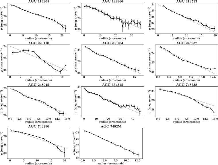
Figure 1. Surface brightness profiles from ellipses fit to r band One Degree Imager (ODI) and partially populated ODI images. Data are shown in black; exponential fits are shown as gray dashed lines.
Download figure:
Standard image High-resolution imageWe masked the images in a semi-automatic fashion, modifying the signal-to-noise threshold for applying masks to nearby sources as appropriate. When in doubt, we chose to be conservative with our masking, not masking features that might be part of the galaxy. We then computed total magnitudes, surface brightnesses, and radii using exponential fits to the resulting profiles; these values are given in Table 2.
Table 2. Observed Optical Properties of H i-bearing Ultra-diffuse Sources
| AGC ID | μg,0 a | reff b | r25 c | g − rd | mr e | Mr f | g | Ag h | Ar i |
|---|---|---|---|---|---|---|---|---|---|
| (mag arcsec−2) | (kpc) | (kpc) | (mag) | (mag) | (mag) | (mag) | (mag) | ||
| 114905 | 23.74 ± 0.13 | 2.99 ± 0.08 | 2.69 | 0.30 ± 0.12 | 18.02 ± 0.09 | −16.47 ± 0.17 | 8.30 ± 0.17 | 0.119 | 0.082 |
| 122966 | 25.65 ± 0.23 | 6.59 ± 0.20 | 3.27 | -0.10 ± 0.22 | 18.47 ± 0.15 | −16.49 ± 0.19 | 7.73 ± 0.12 | 0.273 | 0.189 |
| 219533 | 24.14 ± 0.33 | 3.75 ± 0.13 | 2.05 | 0.12 ± 0.12 | 18.62 ± 0.08 | −16.34 ± 0.23 | 8.04 ± 0.12 | 0.077 | 0.053 |
| 229110 | 24.33 ± 1.70 | 5.26 ± 0.84 | 2.72 | 0.19 ± 0.11 | 18.80 ± 0.08 | −16.47 ± 0.13 | 8.20 ± 0.13 | 0.037 | 0.026 |
| 238764 | 23.76 ± 0.18 | 3.34 ± 0.13 | 2.70 | 0.13 ± 0.11 | 18.87 ± 0.08 | −16.27 ± 0.13 | 8.06 ± 0.12 | 0.074 | 0.051 |
| 248937 | 23.65 ± 0.29 | 4.62 ± 0.28 | 4.40 | 0.23 ± 0.12 | 18.19 ± 0.07 | −17.24 ± 0.12 | 8.54 ± 0.14 | 0.102 | 0.070 |
| 248945 | 23.38 ± 0.35 | 3.83 ± 0.15 | 4.02 | 0.32 ± 0.11 | 17.35 ± 0.07 | −17.32 ± 0.15 | 8.52 ± 0.17 | 0.063 | 0.044 |
| 334315 | 24.74 ± 0.13 | 6.32 ± 0.22 | 0.63 | −0.08 ± 0.18 | 18.23 ± 0.15 | −16.24 ± 0.21 | 7.93 ± 0.12 | 0.223 | 0.154 |
| 748738 | 23.79 ± 0.41 | 1.90 ± 0.13 | 1.56 | 0.16 ± 0.12 | 18.51 ± 0.09 | −15.77 ± 0.21 | 7.89 ± 0.14 | 0.785 | 0.543 |
| 749251 | 23.99 ± 0.18 | 3.01 ± 0.05 | 2.32 | 0.15 ± 0.12 | 19.02 ± 0.08 | −16.20 ± 0.13 | 8.06 ± 0.12 | 0.138 | 0.095 |
| 749290 | 24.75 ± 0.30 | 4.00 ± 0.24 | 1.77 | 0.17 ± 0.12 | 18.18 ± 0.08 | −16.83 ± 0.14 | 8.32 ± 0.13 | 0.108 | 0.075 |

Notes.
a Central surface brightness in the g band, uncorrected for Galactic extinction or surface brightness dimming; obtained by fitting an exponential profile to the observed g band surface density profile. b Effective radius, assuming an exponential profile, derived from the r band surface brightness profile. c Isophotal radius as measured at the 25 mag arcsec−2 isophote. d Color, corrected for Galactic extinction. e Apparent r band magnitude, uncorrected for Galactic extinction or surface brightness dimming. f Absolute r band magnitude, corrected for Galactic extinction, and including a distance error of 5 Mpc. g Stellar mass, estimated from our (Galactic-extinction-corrected) colors and absolute magnitudes, by means of the color–M/L relations from Herrmann et al. (2016). h Galactic extinction correction (Schlafly & Finkbeiner 2011) from the NASA Extragalactic Database in the g band, respectively. i Galactic extinction correction (Schlafly & Finkbeiner 2011) from the NASA Extragalactic Database in the r band, respectivelyDownload table as: ASCIITypeset image
We estimate stellar masses using the color–M/L relation from Herrmann et al. (2016). This relation is calibrated for dwarf irregular-like galaxies, which have many similarities in their stellar properties with field UDGs (though see Du et al. 2020, published after original submission of this work, for a discussion of potential systematic offsets). The uncertainties in our colors, magnitudes, and the color–M/L relation result in Gaussian distributions for each stellar mass estimate; the value reported in Table 2 corresponds to the median of this distribution, and its uncertainties represent the difference of this median with the 16th and 84th percentiles.
3. Results
3.1. The Resolved H i in HUDs
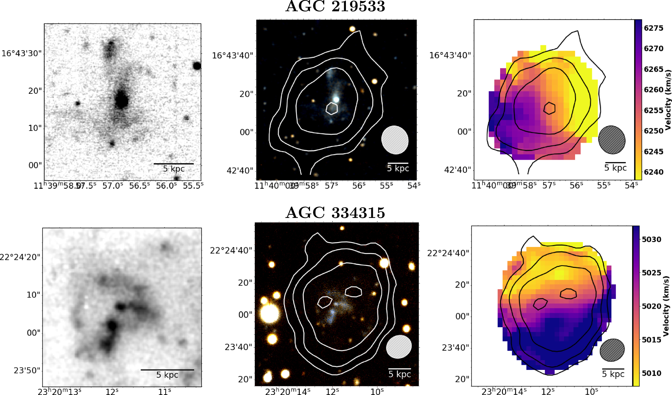
Figures 2–5 show the data for the HUDs in our sample. The central panels show ODI color images of the optical components of the HUDs, with H i column density contours overlaid as white lines, representing contours at the column density levels detailed in the figure captions. The figures are organized in order of ascending peak column density, with galaxies of similar peak column densities grouped with the same contour levels. The left-most column in each figure shows zoomed-in gray-scale g-band ODI images of each galaxy. The right-hand panels show the moment 1 velocity maps, with the black lines representing the same contours as in the optical images. The gray circles represent the size of the beam for each source, and the color gradient represents the line-of-sight velocity in km s−1.

Figure 2. Optical and velocity map comparisons for galaxies AGC 248945, AGC 749251, and AGC 748738 from top to bottom, showing clear velocity gradients across most galaxies and H i gas extending well past the visible optical component. The far left column shows zoomed-in gray scale g-band optical images to show detail. The center column shows color optical images with H i contours overlaid in white, and the right hand column shows H i velocity maps, with column density contours shown in black. The contour overlays represented with the white and black lines in the center and right panels are at column density levels of 0.43, 0.85, 1.7, and 3.4 × 10²⁰ atoms cm−2 for each galaxy. The gray ellipses represent the size of the beam. The R.A. and decl. are in J2000 coordinates.
Download figure:
Standard image High-resolution image
Figure 3. Optical and velocity map comparisons for galaxies AGC 238764, AGC 229110, and AGC 248937. The contour overlays represented with the white and black lines are at column density levels of 1.0, 2.0, 3.0, and 4.0 × 10²⁰ atoms cm−2 for each galaxy. See Figure 2 for details.
Download figure:
Standard image High-resolution image
Figure 4. Optical and velocity map comparisons for galaxies AGC 749290, AGC 122966, and AGC 114905. The contour overlays represented with the white and black lines are at column density levels of 0.56, 1.13, 2.25, and 4.50 × 10²⁰ atoms cm−2 for each galaxy. See Figure 2 for details.
Download figure:
Standard image High-resolution image
Figure 5. Optical and velocity map comparisons for galaxies AGC 219533 and AGC 334315. The contour overlays represented with the white and black lines are at column density levels of 0.81, 1.63, 3.25, and 6.50 × 10²⁰ atoms cm−2 for each galaxy. See Figure 2 for details.
Download figure:
Standard image High-resolution imageIn the H i maps, most sources are resolved with three or four independent beams across the full extent of detected H i emission. Beam sizes range from 145 to 181 in major axis, which corresponds to physical resolutions from 4.6 to 9.1 kpc at the distances of the sources (details listed in Tables 1 and 3).
Table 3. Observed H i Properties of HUDs
| AGC ID | Distance a | V21 b | W50 c | FVLA | log(MH I/M⊙) | a × bd | a × be | σa f | Npeak g |
|---|---|---|---|---|---|---|---|---|---|
| Mpc | km s−1 | km s−1 | Jy km s−1 | arcsec × arcsec | kpc × kpc | kpc | 1020 cm−2 | ||
| 114905 | 76 | 5429.4 ± 0.64 | 34.1 ± 1.6 | 0.94 ± 0.04 | 9.10 ± 0.05 | 29.3 × 26.6 | 10.3 × 9.3 | 1.1 | 5.9 |
| 122966 | 90 | 6517.4 ± 0.90 | 42.5 ± 2.2 | 0.57 ± 0.02 | 9.03 ± 0.05 | 24.5 × 22.1 | 9.9 × 7.8 | 1.3 | 5.6 |
| 219533 | 96 | 6381.5 ± 1.8 | 60.7 ± 5.0 | 0.73 ± 0.04 | 9.24 ± 0.06 | 29.1 × 22.3 | 12.8 × 9.6 | 1.4 | 7.5 |
| 229110 | 112 | 7552.8 ± 1.6 | 45.3 ± 4.2 | 0.36 ± 0.03 | 9.03 ± 0.06 | 18.3 × 14.5 | 8.9 × 5.2 | 1.6 | 5.0 |
| 238764 | 104 | 7010.7 ± 1.6 | 38.5 ± 3.8 | 0.25 ± 0.02 | 8.81 ± 0.06 | 14.4 × 11.3 | 5.9 × 3.9 | 1.5 | 4.8 |
| 248937 | 118 | 8024.54 ± 0.85 | 30.6 ± 2.0 | 0.60 ± 0.04 | 9.29 ± 0.05 | 24.9 × 18.5 | 13.2 × 9.4 | 1.7 | 5.1 |
| 248945 | 84 | 5709.9 ± 1.6 | 47.7 ± 3.9 | 0.37 ± 0.03 | 8.78 ± 0.06 | 17.8 × 14.4 | 6.4 × 4.8 | 1.2 | 4.0 |
| 334315 | 73 | 5108.3 ± 0.52 | 46.4 ± 1.3 | 1.32 ± 0.04 | 9.22 ± 0.05 | 39.1 × 30.6 | 13.4 × 10.0 | 1.0 | 7.3 |
| 748738 | 56 | 3896.5 ± 0.9 | 29.2 ± 2.1 | 0.54 ± 0.03 | 8.61 ± 0.06 | 24.7 × 19.4 | 6.3 × 4.7 | 0.80 | 4.4 |
| 749251 | 106 | 7262.2 ± 0.8 | 33.6 ± 1.9 | 0.38 ± 0.02 | 9.01 ± 0.05 | 17.9 × 15.2 | 8.1 × 6.5 | 1.5 | 4.1 |
| 749290 | 97 | 6512.5 ± 1.0 | 42.7 ± 2.5 | 0.40 ± 0.02 | 8.95 ± 0.05 | 19.8 × 15.4 | 8.3 × 6.1 | 1.4 | 5.2 |
Notes.
a Distances calculated from ALFALFA flow model (see Haynes et al. 2011). b H i recessional velocity measured at 50% of the peak flux; errors are statistical errors from the fit. c H i line width measured at 50% of the peak flux; errors are statistical errors from the fit. d Semimajor and semiminor axis of the H i measured at a column density of 1.25 × 10²⁰ atoms cm−2 as discussed in the text. DH I is 2 × a. e Semimajor and semiminor axis as in note d, converted to physical units using the assumed distance. f Uncertainty in the semimajor axis, in physical units. Uncertainties for the semiminor axis are similar. g Peak column density measured in the moment 0 images.Download table as: ASCIITypeset image
Sources AGC 238764 and AGC 248945 are only marginally resolved, with measured H i semimajor axes at 1 M⊙ pc−2 equal to or less than the beam size, and with only around two beams across the full detected extent of the galaxies. These two sources are also the only two with recovered fluxes FVLA/FALFA well below 1 (0.55 and 0.59 respectively).
Most HUDs in our sample appear to have regular H i gas morphologies. While this is to be expected at our relatively low physical resolution, it indicates these sources are not likely disturbed clouds of debris, and are presumably disks, allowing for reasonable estimates of the inclinations of these HUDs, which we discuss further in Section 4.1.
All HUDs presented exhibit H i gas distributions that extend well beyond their observed optical counterparts. This is characteristic of typical H i-bearing galaxies (e.g., Boomsma et al. 2008; Lelli et al. 2016), but is interesting given the extended "ultra-diffuse" nature of the stellar populations in question. We return to this point in Section 4.2. We also find that the gas is most dense in the center of these galaxies and becomes less dense as the H i radius increases from the center. Peak H i surface densities range from 3.98 to 7.50 × 10²⁰ atoms cm−2, though it is important to note that this measurement assumes the gas fills the beam, and thus depends heavily on our resolution; the true peak density is almost certainly higher.
We estimate the H i diameter at an H i surface density of 1 M⊙ pc−2 along the major axis using a second-moment analysis method, as described in Banks et al. (1995). Specifically, we measure the elliptical shape of emission above the 1 M⊙ pc−2 level by applying a column density threshold of 1.25 × 10²⁰ atoms cm−2 to the moment 0 map. We then calculate the first- and second-order moments of the 3'' pixels at or above the threshold, which we then use to calculate the position angle and major and minor axes of the resulting fitted ellipse. Following Wang et al. (2016), we then correct the major axis diameter for beam smearing by

and perform an analogous correction for the minor axis to obtain the final values for the H i sizes of our sources. The H i radii measurements range from 6.7 to 13.9 kpc along the major axis; details are reported in Table 3 for each source.
The right-hand panels in Figures 2–5 show the derived moment 1 maps, representing the velocity field for the galaxies in our sample, with the same total flux column density contours from the center panels overlaid in black to allow for direct comparison. 7 We see velocity gradients and evidence of ordered rotation in the moment 1 maps for all of the sources. While there is little evidence for irregular motions in their H i gas, some sources (e.g., AGC 248945 and AGC 334315) have very regular gradients, while others (e.g., AGC 749251 and AGC 748738) show gradients that are somewhat less regular, though the low resolution of our images does not allow for a more detailed analysis. In most cases, the orientation of the velocity gradient appears aligned along the H i major axis though, in three cases (AGC 229110, AGC 749251, AGC 749290), there is a moderate offset in measured position angles based on the kinematics and the morphology (see Section 4.1).
Gaussian fitting to the global H i line profiles extracted from the data cubes gives measured line widths for the HUDs that range from 29.2 to 47.6 km s−1, as listed in Table 3. As noted in Leisman et al. (2017), these velocity widths are lower than typically seen in galaxies of similar mass; Mancera Piña et al. (2019b, 2020) show that, when corrected for inclination (Section 4.1), these sources fall off the BTFR (e.g., McGaugh et al. 2000; McGaugh 2005).
3.2. The Stellar Populations of Resolved HUDs
The left-hand and center panels in Figures 2–5 show the optical data for the 11 galaxies in our sample. The left-hand panels are g-band images with contrast chosen to highlight the low surface brightness features of the galaxies, while the center panels show color images with H i contours at column density levels based on peak column density overlaid in white.
All sources have very low surface brightness, with clearly detected stellar features that are nearly invisible in SDSS imaging. Similar to the result reported in Leisman et al. (2017), most HUDs appear blue in color with mostly irregular morphologies without well defined features. Two sources, AGC 334315 and AGC 749251, have some arc-like features reminiscent of spiral arms, but without distinct patterns or strong evidence of a stellar disk. Three sources, AGC 114905, AGC 748738, and AGC 749290, have observed optical components that loosely resemble stellar disks in our optical images, but still would be better classified as irregular galaxies at the detected level. Also, one source, AGC 219533, has a bright, very blue higher surface brightness clump superimposed on its low surface brightness emission; it is not fully clear whether it is a bright star-forming region associated with the galaxy, or if it is a foreground or background source.
In many cases the centroid of the stellar population is aligned with the peak in the H i column density, but there are several exceptions, including AGC 114905, AGC 238764, and AGC 248945. However, we note that AGC 238764 and AGC 248945 are less well resolved and have lower signal-to-noise detections than the other sources in the sample, so the position of their peak column density is somewhat less well defined.
Importantly, we note that we only poorly constrain the galaxies' inclinations using the stellar populations. Part of this is that the irregular morphologies make it difficult to accurately estimate the structural parameters used to constrain inclination and construct surface brightness profiles (Section 2.2). While the process of azimuthally averaging the light tends to mitigate the effect of these structural uncertainties on the measurements of magnitude, surface brightness, and effective radius (especially as we hold the position angle and axial ratio fixed), these uncertainties strongly affect the reliability of estimates of the major and minor axis. Moreover, the patchiness of the stellar light suggests that it may not be true that the apparent axial ratio of the light from the most visible stars actually traces the stellar disk, thus only providing at best a loose constraint on the systemic inclination. Only three of the sources have morphologies that loosely resemble stellar disks, AGC 114905, AGC 748738, and AGC 749290; for these three sources we find that attempts to measure their inclination optically always differs considerably from the value found using the H i gas. Additionally, we note a significant difference between the optical and H i position angles in AGC 749290. We come back to these points and their implications in Section 4.1.
3.3. H i Mass–Diameter Relation
The H i mass–diameter relation is an observed tight correlation between the H i mass of a galaxy and its H i radius measured at an isophotal level of 1 M⊙ pc−2 (e.g., Broeils & Rhee 1997; Lelli et al. 2016; Wang et al. 2016). Given that the HUDs are selected to have extended optical counterparts, it is a natural question to ask if they also have extended H i disks for their mass. Indeed, we may expect HUDs to fall off the relation, having larger H i sizes for their mass if the formation mechanism responsible for their extended optical size also affects the gas disk (though the physical interpretation of the H i mass–diameter relation is complex; see, e.g., Stevens et al. 2019). If any of the HUDs are "failed" L⋆ galaxies (e.g., van Dokkum et al. 2015, 2016), an extended gas disk could help to explain their low surface brightness nature: an extended H i disk for a given H i mass implies a lower average surface density of gas, which could affect the ability of the neutral gas to condense and cool to form stars (e.g., Bacchini et al. 2019). The H i maps presented in Section 3 are sufficiently resolved to begin to address this question, with the H i disks typically resolved with two to five resolution elements across the whole disk.
Figure 6 shows the MH I–DH I relation from Wang et al. (2016), with a red solid line indicating the linear fit to their relation

and with dashed lines showing their estimated 3σ scatter (σ ∼ 0.06 dex) around the mean relation. Yellow stars show the HUDs from our sample plotted on the relation, with errors in the H i diameters statistically estimated to be approximately 6'' (the size of two pixels). These sources all fall on the relation; despite being selected for extended optical sizes, their H i disks are indistinguishable from other galaxies of similar H i mass.
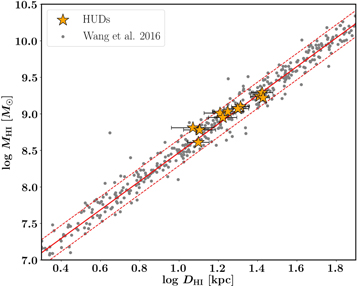
Figure 6. DH –MH relation, with the H i-bearing ultra-diffuse galaxies (HUDs) overplotted on data from Wang et al. (2016). The HUDs, despite having an extended, "ultra-diffuse" stellar population, are H i normal, with typical H i radii and global gas densities. The solid line shows the linear fit from Wang et al. (2016). The dotted lines show the 3σ scatter around the relation. H i mass errors are smaller than the size of the markers.
Download figure:
Standard image High-resolution imageWe note that the H i masses in this plot are measured from the VLA flux, which was consistent with the ALFALFA flux for all but two sources, as discussed in Section 3.1. If one instead uses the single-dish fluxes for AGC 238764 and AGC 248945, they move up slightly (∼0.2 dex), making them just barely consistent with the relation.
We interpret this result further in Section 4.2.
4. Discussion
Here we discuss our results, noting the importance of resolved H i imaging for measuring inclinations, H i radii, and column densities, as well as deep optical imaging for measuring optical sizes at low surface brightness. We explore the implications of the ultra-diffuse sources falling on the MH I–DH I relation, finding that though their stellar disks have extremely low surface brightness, and though they are dark matter poor inside their disks (Mancera Piña et al. 2019b), their H i radii are typical for their optical effective radii. However, their H i radii are large for their stellar mass, suggesting these galaxies are quite gas rich, consistent with the findings from Leisman et al. (2017).
4.1. H i Inclination Measurements
One of the main results from this sample, presented in detail in Mancera Piña et al. (2019b) is that these isolated, very low surface brightness sources appear to be rotating too slowly for their baryonic mass, i.e., they lie off the BTFR. Leisman et al. (2017) found low velocity widths for the larger parent sample, but resolved measurements are necessary to constrain the source inclinations and ensure against inclination selection bias.
A number of methods can be employed for measuring the inclination of galactic disks (see, e.g., Garcia-Gomez & Athanassoula 1991; Andersen & Bershady 2013). Mancera Piña et al. (2019b) determine inclinations by minimizing the residuals between observed moment 0 maps and model galaxies projected across a range of inclinations, including a convolution step that makes the measurement of the inclination largely unbiased by the shape of the beam (see Mancera Piña et al. 2020 for a detailed description).
Another common method is to use ellipses fit to 2D H i or optical photometric images to derive position angles and axial ratios, which are then converted to inclination assuming disks of some estimated thickness (see e.g., Boroson 1981). In the cases where the minor axis of our galaxies is resolved with at least two beams, we estimate axial ratios with our beam corrected major and minor axis measurements, and use these to compute inclinations using the standard formula (e.g., Jacoby et al. 1992)

assuming two representative values for thin and thick disks, q0 = 0.1 and 0.4. We report these, along with the measurements from Mancera Piña et al. (2019b), in Table 4. For the galaxies included in both samples, our measurements are consistent with those derived from Mancera Piña et al. except in two cases: AGC 248945 and AGC 334315. These two galaxies had inclinations that were more than 10° different (smaller) from those found in Mancera Piña et al., though are still within 2σ given uncertainties due to beam smearing.
Table 4. H i Morphological Parameters
| AGC ID | H i PA a | H i i0.1 b | H i i0.4 c | H i iMP d | Enclosed e |
|---|---|---|---|---|---|
| Degrees | Degrees | Degrees | Degrees | Fraction | |
| 114905 | 79 | 26 ± 19 | 28 ± 19 | 33 ± 5 | 0.86 ± 0.04 |
| 122966 f | 67 | 39 ± 15 | 43 ± 15 | 34 ± 5 | 0.87 ± 0.05 |
| 219533 | 138 | 41 ± 12 | 46 ± 12 | 42 ± 5 | 0.85 ± 0.04 |
| 229110 f | 142 | 54 ± 15 | 62 ± 15 | ⋯ | 0.77 ± 0.07 |
| 238764 | 27 | 48 ± 23 | 54 ± 23 | ⋯ | 0.76 ± 0.08 |
| 248937 f | 22 | 44 ± 13 | 49 ± 13 | ⋯ | 0.83 ± 0.06 |
| 248945 | 268 | 41 ± 20 | 46 ± 20 | 66 ± 5 | 0.78 ± 0.07 |
| 334315 | 165 | 41 ± 8 | 46 ± 8 | 52 ± 5 | 0.91 ± 0.03 |
| 748738 | 30 | 41 ± 14 | 45 ± 14 | ⋯ | 0.74 ± 0.05 |
| 749251 | 5 | 36 ± 23 | 40 ± 23 | ⋯ | 0.72 ± 0.08 |
| 749290 | 118 | 44 ± 17 | 49 ± 17 | 39 ± 5 | 0.79 ± 0.06 |
Notes.
a Position angle estimated from the H i morphological fitting. Uncertainties in the position angles are ∼6°. b Morphological inclination estimated from the H i axial ratio assuming q0 = 0.1. c Morphological inclination assuming q0 = 0.4 d Inclination estimates from Mancera Piña et al. (2019b). e The fraction of H i flux within the measured H i radius. f For these galaxies the observed morphological axis does not coincide with the rotational gradient; the inclination estimates assuming nicely rotating disks should be treated with cautionDownload table as: ASCIITypeset image
We find that the estimated inclinations for our 11 sources tend to cluster around 40°, ranging only from 26° to 54°. Though our inclinations are only somewhat weakly constrained due to our comparatively low resolution, these constraints still give physically interesting results. First, this inclination distribution seems inconsistent with the assumption of randomly oriented oblate spheroids. More specifically, we would expect randomly oriented oblate spheroids to be evenly distributed in bins of (that is, for the number of galaxies in each inclination bin to increase from face on (0°) to edge on (90°) as a function of ; see, e.g., Binney & Merrifield 1998). This distribution can be modified somewhat by diameter and magnitude selection effects (e.g., Jones et al. 1996), though these effects are modest for optically thin disks. Even with just 11 sources, our measured inclinations seem inconsistent with a random distribution (even accounting for magnitude or diameter selection effects); a Kolmogorov–Smirnov (KS) test gives a probability that the sources in our sample have a random underlying distribution of p < 0.001.


That our galaxies are not randomly distributed is in itself not surprising: the surface brightness criteria used in Leisman et al. (2017), along with the visual elimination of sources, could easily bias the sample against edge-on galaxies. This may in part explain our observed distribution.
However, while these results may suggest an inclination-dependent selection bias in Leisman et al. (2017) and Janowiecki et al. (2019), they also support the conclusion that their observed low velocity width distribution for the full sample of HUDs cannot be explained by inclination effects. A KS test comparing our observed inclination distribution with the distribution necessary to make the Leisman et al. (2017) HUDs lie on the BTFR gives a probability p = 9 × 10⁻⁷ of being drawn from the same distribution. This result thus supports the argument from Mancera Piña et al. (2019b) that HUDs indeed do have abnormally low rotation velocities for their mass.
Yet, it is also possible that our observed inclination distribution indicates that the assumption of thin oblate spheroids may not be appropriate for this sample of galaxies. A number of authors (e.g., van den Bergh 1988) have pointed out that dwarf irregular galaxies may not be well represented by spheroids with some intrinsic flattening, and may rather be triaxial, or at least have thicker disks. While the freefall time for H i makes a thick H i disk unlikely, a triaxial or otherwise irregular disk may be reasonable in light of their irregular stellar properties. Thus, we emphasize the importance of caution when approaching inclination measurements for these extreme sources.
As a further note of caution, we compare the H i inclination estimates to estimates of optical inclination. As discussed in Section 3.2, most sources in our sample have irregular optical morphologies, precluding accurate optical measurements of inclination. However, for the three sources with the most regular morphologies in our sample, AGC 114905, AGC 748738, and AGC 749290, we estimate stellar inclinations to compare to our H i measurements. In all three cases, the inclination estimate from the stellar population is ∼20° different from the estimates from H i, with the stellar disk giving larger inclinations than the H i (which, we note, would place them even further off the BTFR). We find the offsets in the HUDs sample are even more extreme than those in Verheijen & Sancisi (2001), who also found a significant difference between inclinations measured optically, and using H i.
Further, there appears to be a 90° difference between the position angle measurements for AGC 749290 with the optical being 289° and H i being 28°. These differences may be because the observed optical morphology in HUDs is likely dominated by patchy star formation. Therefore, we reiterate that the stellar population of H i-bearing UDGs is, in general, a poor indicator of inclination; we must also consider the H i component when attempting to understand the orientation of HUDs.
This note is especially important given the draw to inclination selection of edge-on HUDs (e.g., He et al. 2019), since this, in principle, removes the problem of inclination correction for rotational (and surface brightness) studies. Since HUDs are likely a heterogeneous population including both irregular and spiral-like disks, it may or may not be that sources with high axial ratios are edge-on disks where inclination corrections can be ignored. Our work confirms that the optical morphologies are not necessarily aligned with the kinematics of the gas, so one should exercise caution in interpreting unresolved kinematic information.
4.2. Implications of HUDs on the H i Mass–Diameter Relation
The results presented in Section 3.3 and Figure 6 show that the HUDs in this sample are all consistent with the H i mass–diameter relation of Wang et al. (2016). Another way of exploring this result is to calculate the average H i surface density for our sample, which should give a result similar to other H i-bearing galaxies, regardless of mass. Following Broeils & Rhee (1997), we compute a characteristic surface density , which is slightly higher than, but consistent with, their value of 3.8 ± 0.1 M⊙ pc−2. 8 Like other authors, we note that this characteristic ΣH I,c is actually slightly higher than the actual average ΣH I, because we use the full measured MH I rather than MH I enclosed within DH I to most accurately compare with previous works.

Given the lower stellar surface density of these sources, the "normal" H i surface density may be somewhat surprising (e.g., de Blok & McGaugh 1996). One potential explanation is that the H i radii are isophotal radii, measured at one position along the surface density profile, whereas the effective radius measurement used to define the optical radius is related to the slope of the light profile. Thus, these sources could still have larger than typical effective H i radii if they have shallower slopes.
We explore this by measuring the flux enclosed within the H i radius, compared with the flux outside the radius. We compute the fraction of the total flux enclosed within the H i radius, and report the values in Table 4. We find that our sources contain an average of ∼81% of the total H i flux within the measured H i radius, with a sample standard deviation 6% (though we note the individual uncertainties based on the rms in our flux measurements are typically closer to 10%). This is consistent with the estimates from Wang et al. (2016) of ∼83% ± 10%.
We also confirm that this technique can differentiate between samples with different slopes by applying this method to nine ATLAS 3D (Serra et al. 2012) sources used in the Wang et al. (2016) sample which have significantly shallower H i profiles (see their Figure 2). We find that these galaxies contain an average of 62% of the total H i flux within the H i radii reported in Wang et al., with a standard deviation of 14% (though we note that this comparison is somewhat limited since a number of the ATLAS 3D sources are disrupted, making estimation of the H i radius more difficult (see Serra et al. 2012, 2014).
To determine whether our masking procedure introduces a systematic bias, we also compute this enclosed fraction on our unmasked cubes. We find this decreases our average measured gas fraction to 76% ± 9%, though most of this change is driven by two sources with additional positive flux at large radii in the unmasked cubes, which changes their estimated gas fractions by ∼16%. If we remove these sources the average value is 79% ± 6%. Though it provides a less direct comparison, we also note that we recover, on average, 96% of the ALFALFA flux, so if we instead use ALFALFA fluxes, this could further decrease the gas fraction by an average of ∼4%, still consistent with, but lower than, the value measured by Wang et al. (2016).
Thus, we suggest that the consistency of our measured enclosed fractions with Wang et al. (2016) implies that the slope of the H i profiles is not significantly different from typical H i-bearing sources. However, higher-resolution, well resolved H i profiles will be necessary to confirm this result.
We also explore measuring optical isophotal radii for this sample of galaxies, and present the radii measured at 25 mag arcsec−2 in the r band in Table 2. However, while for typical gas-bearing galaxies radii measured at 25 mag arcsec−2 contain most of the optical light, for our galaxies, with peak surface brightness near 24 mag arcsec−2, this estimate misses most of the light of the galaxy. In fact, while for typical galaxies r25 is 3–5× larger than the effective radius (i.e., the radius containing half the light), for our sources we find that r25 is approximately 2/3 of the effective radius (). This means that for our sample, measurements of RH I/ropt,25 are significantly elevated compared with other samples. We find 〈RH I/ropt,25〉 = 5.1 ± 1.6, compared to, e.g., 1.7 ± 0.5 as measured by Broeils & Rhee (1997) for spiral galaxies, or 1.9 ± 1.0 from Lelli et al. (2016) for the SPARC sample (disk galaxies).

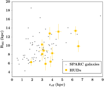
If instead we compare H i radii to optical effective radii, we find the effective radii are only somewhat larger than predicted by their H i extent. Figure 7 shows the H i radii compared with the stellar effective radii for our sample and the SPARC sample of disk galaxies (Lelli et al. 2016), selected to have the same H i mass range (though a much larger stellar mass range). The HUDs fall in a similar parameter space, though with an elevated average effective radius (matching their initial selection). This is understandable, given that Leisman et al. (2017) reported that these sources all have larger than usual gas fractions (see, e.g., their Figure 4).
Figure 7. H i radius (measured at 1 M⊙ pc−2) vs. optical effective radius for our sample (yellow squares), compared with disk galaxies from the SPARC sample (Lelli et al. 2016). The SPARC galaxies are selected to have the same H i mass range, but have a wide range of stellar masses. The HUDs have elevated, but not extreme, stellar effective radii from an H i perspective.
Download figure:
Standard image High-resolution image
Thus, when considered from the H i perspective, our sample of HUDs appears H i normal at our current resolution, with slightly elevated stellar radii, but very small stellar masses and low surface brightnesses. HUDs do not significantly differ from typical galaxies in their average H i surface densities and, at the resolution of our data, appear to have normal H i gas distributions. While higher-resolution observations will be required to confirm the full mass–density profiles of these galaxies, the results presented here suggest that, though their stellar populations are ultra-diffuse, the H i gas in HUDs is not.
5. Conclusions
In this paper we present deep optical and resolved H i imaging of a sample of 11 isolated H i-bearing ultra-diffuse galaxies selected from the ALFALFA survey. These sources are notable because of their extreme low surface brightnesses, large optical sizes, and their relative isolation from other sources.
We find that the sources have irregular optical morphologies with generally blue colors, consistent with the findings in Leisman et al. (2017). We note that the stellar populations in these irregular sources, perhaps not unexpectedly, often give inconsistent inclination measurements with the H i; thus resolved H i measurements are essential for inclination-dependent studies. However we also caution that our observed inclination distribution seems inconsistent with a random distribution, potentially due to selection effects, or H i distributions that deviate from circular disks.
We further find that, at the level of our resolution, the sources in this sample appear to have normal H i morphologies, with the H i extending beyond the observed diffuse stellar population in all cases.
We plot these extreme sources on the MH I–DH I relation, and find that they are all consistent with the relation, and that they have normal global H i surface densities. We explore the gas fraction enclosed within the H i radius, and find it consistent with normal H i disks, suggesting that though their stellar populations are ultra-diffuse, the H i in HUDs is not. This suggests that, globally, their extreme surface brightness may not be driven by low or anomalous H i densities or distributions, though higher-resolution observations will be necessary to confirm this suggestion.
This publicly available, 9 rich data set provides an important baseline for future exploration of these mechanisms and other questions relying on resolved studies of HUDs (e.g., their dark matter content; Mancera Piña et al. 2019b), and for direct comparisons between theoretical models and observations.
The authors acknowledge the work of the entire ALFALFA collaboration in observing, flagging, and extracting sources, and would like to thank the anonymous referee for useful suggestions that improved the quality of the paper. The ALFALFA team at Cornell has been supported by grants NSF/AST 0607007, 1107390 and 1714828 and by the Brinson Foundation. P.E.M.P. and F.F. are supported by the Netherlands Research School for Astronomy (Nederlandse Onderzoekschool voor Astronomie, NOVA), Phase-5 research program Network 1, Project 10.1.5.6. E.A.K.A. is supported by the WISE research program, which is financed by the Netherlands Organization for Scientific Research (NWO). Worked carried out by N.J.S., H.J.P., and K.L.R. for this project is supported by NSF grant AST-1615483. L.G. and L.L. acknowledge support from Valparaiso University. K.R. and L.L. acknowledge support from NSF/AST-1637339.
J.M.C. is supported by NSF/AST-2009894. J.M.C. and Q.S. acknowledge support from Macalester College.
This work is based in part on observations made with the VLA, Arecibo Observatory, and WSRT. The VLA is a facility of the National Radio Astronomy Observatory (NRAO). NRAO is a facility of the National Science Foundation operated under cooperative agreement by Associated Universities, Inc. The Arecibo Observatory is operated by SRI International under a cooperative agreement with the National Science Foundation (AST-1100968), and in alliance with Ana G. Mèndez-Universidad Metropolitana, and the Universities Space Research Association. The Westerbork Synthesis Radio Telescope is operated by the ASTRON (Netherlands Institute for Radio Astronomy) with support from NWO.
Observation presented in this paper were obtained with the WIYN Observatory, which is a joint facility of the NSF's National Optical-Infrared Astronomy Research Laboratory, Indiana University, the University of Wisconsin-Madison, Pennsylvania State University, the University of Missouri, the University of California-Irvine and Purdue University.
Footnotes
- 7
We note that the velocity maps are masked on smoothed images, which means that some of the noise outside the lowest signal-to-noise contour is displayed in each image.
- 8
Broeils & Rhee (1997) report a standard deviation of 1.1 which, for their sample of 108 galaxies, gives a standard error on the mean of 0.11. The error on our characteristic surface density of 0.27 is the standard error on the mean.
- 9
Final reduced H i and optical data products are available at https://scholar.valpo.edu/phys_astro_fac_pub/186/.