


Abstract
Horizon Run 5 (HR5) is a cosmological hydrodynamical simulation that captures the properties of the universe on a Gpc scale while achieving a resolution of 1 kpc. Inside the simulation box, we zoom in on a high-resolution cuboid region with a volume of 1049 × 119 × 127 cMpc3. The subgrid physics chosen to model galaxy formation includes radiative heating/cooling, UV background, star formation, supernova feedback, chemical evolution tracking the enrichment of oxygen and iron, the growth of supermassive black holes, and feedback from active galactic nuclei in the form of a dual jet-heating mode. For this simulation, we implemented a hybrid MPI-OpenMP version of RAMSES, specifically targeted for modern many-core many-thread parallel architectures. In addition to the traditional simulation snapshots, lightcone data were generated on the fly. For the post-processing, we extended the friends-of-friend algorithm and developed a new galaxy finder PGalF to analyze the outputs of HR5. The simulation successfully reproduces observations, such as the cosmic star formation history and connectivity of galaxy distribution, We identify cosmological structures at a wide range of scales, from filaments with a length of several cMpc, to voids with a radius of ∼ 100 cMpc. The simulation also indicates that hydrodynamical effects on small scales impact galaxy clustering up to very large scales near and beyond the baryonic acoustic oscillation scale. Hence, caution should be taken when using that scale as a cosmic standard ruler: one needs to carefully understand the corresponding biases. The simulation is expected to be an invaluable asset for the interpretation of upcoming deep surveys of the universe.
Export citation and abstract BibTeX RIS
1. Introduction
Understanding the cosmic origin of the observed diversity of galaxies is an interesting and challenging problem. While baryonic matter accounts for only about 5% of the energy budget of the universe, its impact on galaxy formation is critical and must be accounted for statistically. Over the last decade, a plethora of cosmological simulations reaching typically kiloparsec resolution have been produced to address this challenge, e.g., MareNostrum (Ocvirk et al. 2008), Horizon-AGN (Dubois et al. 2014b), Illustris (Genel et al. 2014), MassiveBlack-II (Khandai et al. 2015), EAGLE (Schaye et al. 2015), Magneticum (Dolag et al. 2016), Romulus (Tremmel et al. 2017), BAHAMAS (McCarthy et al. 2017), IllustrisTNG (Marinacci et al. 2018; Naiman et al. 2018; Nelson et al. 2018, 2019; Pillepich et al. 2018b; Springel et al. 2018), and SIMBA (Davé et al. 2019). They aim to model as accurately as possible the intricate physical processes occurring on multiple scales, either by resolving them (using refinement techniques) or using so-called subgrid models. They track the full cosmic history of what aims to be a statistically representative region of the universe using hydrodynamics and gravity, and typically account for gas cooling, star formation, and stellar and active galactic nuclei (AGNs) feedback as well as metal production, in order to provide statistical insights into a wide range of astrophysical problems.
We are also fortunate to live in the age of existing and forthcoming very large photometric (e.g., SXDS (Sekiguchi & SXDS Team 2004), COSMOS (Scoville et al. 2007), Alhambra (Moles et al. 2005), DES (Sánchez et al. 2014), Euclid (Laureijs et al. 2011), HSC (Aihara et al. 2018a), and LSST (LSST Dark Energy Science Collaboration 2012)) and spectroscopic surveys (e.g., 4MOST (de Jong et al. 2012), JPAS (Benitez et al. 2014), WFIRST (Spergel et al. 2013), DESI (DESI Collaboration et al. 2016), MSE (McConnachie et al. 2016), and PFS (Aihara et al. 2018b)),13 allowing us to probe not only our present-day universe, but also a significant period of cosmic time.
The confrontation of the cosmological simulations with galaxy surveys has been very successful at reproducing a significant number of features. Examples include studies of the amplitude of galaxy clustering, the morphology and topology of large-scale structures (Park 1990; Park et al. 2005, 2012; Choi et al. 2010), the cosmic evolution of the star formation rate and luminosity function (e.g., Devriendt et al. 2010), and the bimodality of the physical, spectroscopic, and morphological properties of galaxies at low redshift (e.g., Dubois et al. 2016), while probing a diversity of environments and epochs. Nonetheless, compared to the observed universe, one of the main limitations of past cosmological hydrodynamical simulations has been the dynamical range of scales probed.
Recent examples of simulations of entire cosmological volumes, such as Horizon-AGN, the TNG100 run of the IllustrisTNG project, or Eagle, can capture scales ranging from ∼100 Mpc to 1 kpc. This is rather restrictive, both from a statistical standpoint—rare events are quite sensitive to the underlying cosmological parameters—as well as from a physical standpoint. In particular, the large-scale peculiar velocity field cannot be properly recovered for many cosmological models, such as the popular ΛCDM model, in such small-volume simulations. Furthermore, the gravity and baryonic processes couple over widely different scales (as can be seen in intrinsic alignments, or in the strangulation of dwarfs in clusters). When improperly accounted for, this can in turn impact dark energy experiments (e.g., Chisari et al. 2018), among others. Indeed, one significant shortcoming of most past simulations is to underestimate the observed spread in the properties of cosmic structures (e.g., colors, V/σ etc.), which could be due to simulators calibrating their subgrid physics on the mean of the observed process (and not accounting for its full variance), but could also be a consequence of the lack of diversity of the underlying physics captured in small boxes (such as the lack of rare events). For instance, the mean separation of rich clusters is known to be ∼ 70 cMpc and ∼ 40 cMpc for quarsi-stellar objects (QSOs; Bahcall & West 1992), indicating that only a few dense environments and QSOs are contained in a cosmological volume with a side length of 100 cMpc. Furthermore, Colombi et al. (1994) show that a two-point correlation function begins to deviate from theory when the separation scale is larger than one-fifth of the simulation box size. Therefore, one may need simulations with a volume larger than hundreds of cMpc on a side in order to examine the distribution of galaxies on the baryonic acoustic oscillation (BAO) scale, and to capture a wide range of environments.
The Horizon Run series of cosmological simulations (Kim et al. 2009, 2011, 2015) have adopted large volumes (84–3390 cGpc3) in order to grasp the important large-scale properties of the cosmological models under study, as well as to secure large statistical samples for quantitative comparisons between observations and simulations. The Horizon Run 5 (HR5) simulation14 presented in this paper, being the first hydrodynamic simulation in this series, follows the idea of the previous generations of the Horizon Runs. HR5 is able to capture physical processes on scales ranging from Gpc down to kpc scales, with a dynamic range an order of magnitude greater than any previous simulations of this kind. The total volume of the high-resolution region is ∼2 times smaller than the largest TNG300 simulation of the IllustrisTNG project (Springel et al. 2018) with slightly better resolution. However, the true strength of HR5 is that the length of the simulation box will give us access to the long-wavelength modes of the density power spectrum up to 1 cGpc. This is something that has not previously been achievable in hydrodynamic simulations that are also capable of resolving galactic processes.
As discussed in more detail below, the geometry of the simulation was chosen to provide a means of easily extracting virtual lightcones from the data. These can easily be used for Lyα tomography, and more generally to study the large-scale chemical properties of the IGM. Compared to other hydrodynamical simulations, the wide range of scales probed by HR5 provides us with a large-scale peculiar velocity field consistent with the underlying cosmological model, as well as a fair sample of massive clusters. It also allows us to probe the impact of the very large-scale structures (wall, filaments, voids) on galaxy formation, clustering, and weak lensing. In particular, the simulation was customized to probe BAO scales, the impact of large-scale streaming velocity, velocity bias, and intrinsic alignments. This is achieved by setting up initial conditions that reflect the expected excess power at the relevant scale. The simulation's cosmic variance is also set to obey that of the universe on gigaparsec scales, which allows us to study the formation of massive clusters and the most massive SMBH they host in a realistic environment. We implemented a bipolar jet model for AGN feedback coupled to black hole (BH) spin, which aims to better model the energy deposition on kpc scales. We also included detailed chemistry (including oxygen and iron) for the IGM in order to answer astrophysical problems, such as the missing baryon problem. At a technical level, we made use of a power spectrum generated by CAMB (Howlett et al. 2012) to generate distinct velocity fields for the dark matter and baryons, and implemented OpenMP parallelization in order to make better use of modern multicore computing architectures.
In the following paper, we will present the main characteristics of the simulation in Section 2, while Section 3 describes the subgrid physics prescriptions incorporated into the simulation code. Section 4 presents the type of raw data produced in the simulation suite. Section 5 presents the suite's dark matter halos and large-scale structure properties. In Section 6, we present our results with regard to the global stellar properties of the simulation. Finally, we will present our conclusions in Section 7.
2. Simulations
We will first describe the numerical code used for HR5 (Section 2.1) before focusing on the generation of the zoomed initial conditions (Section 2.2). We will then discuss the OpenMP optimization (Section 2.3) and the output strategy. Finally, sister simulations with slightly different subgrid physics will be described in Section 2.4.
2.1. Numerical Setup
The simulations were carried out using the adaptive mesh refinement code RAMSES (Teyssier 2002). To solve for gravity, the dark matter, star, and BH particles masses are projected onto the grid with a cloud-in-cell assignment scheme. The grid mass density (together with the contribution of the gas) is used to compute the gravitational acceleration through the Poisson equation solved with a multigrid relaxation method. Particles are evolved through time using leapfrog integration. The grid is adaptively refined in the zoom-in region using a quasi-Lagrangian criterion: wherever the mass is larger (smaller) than eight times that of the high-resolution dark matter/baryonic resolution, the cell is refined (or derefined) up to a best achieved resolution of 1 physical kpc. To achieve a nearly constant physical maximum resolution in a comoving box, a new level of refinement is added at expansion factors aexp = 0.0125, 0.025, 0.05, 0.1, 0.2, 0.4, and 0.8, where the present epoch is defined by aexp = 1. The time step is adaptive, with a shared step size across a given refinement level, and varies by a factor of 2 across contiguous levels. The minimum step size is determined by the Courant condition, with a Courant factor of C = 0.8.
The hydrodynamics is solved directly on the grid, rather than by evolving particles whose potential and acceleration are computed using the grid. The set of Euler equations is solved with the unsplit MUSCL-Hancock method (van Leer 1979): fluxes are obtained with a second-order Godunov scheme using the approximate Harten–Lax–van Leer contact wave (Toro et al. 1994) Riemann solver, and the minmod slope limiter on conservative variables. The gas is assumed to be of primordial composition, with a hydrogen fraction of XH = 0.76. The remaining gas is assumed to be composed of helium, and the mixture follows the ideal equation of state of a mono-atomic gas with adiabatic index of γ = 5/3.
The simulation probes the large-scale structures residing in a cubic volume of (1049 cMpc)3 with the highest-resolution elements measuring 1 kpc in size. In order to both take advantage of the high resolution and sample the very large-scale structures, we defined an elongated cuboidal zoom region whose length is 1049 cMpc and whose rectangle cross section measures 119 × 127 cMpc2. Outside the zoom region, the low-resolution elements account for the influence from the large-scale structure. This unique zoom-in geometry was adopted to optimize the construction of a lightcone in order to facilitate a direct comparison with existing and upcoming surveys of the deep universe, e.g., COSMOS (Scoville et al. 2007), DES (Sánchez et al. 2014), LSST (LSST Dark Energy Science Collaboration 2012), and DESI (DESI Collaboration et al. 2016).
2.2. Cosmology and Initial Conditions
The cosmological parameters are compatible with Planck data (Planck Collaboration et al. 2016), with Ωm = 0.3, ΩΛ = 0.7, Ωb = 0.047, σ8 = 0.816, and h0 = 0.684, and the linear power spectrum is calculated from the CAMB package (Lewis et al. 2000). The simulation initial conditions at z = 200 are generated with the MUSIC package (Hahn & Abel 2011) using second-order Lagrangian perturbation theory (2LPT; Scoccimarro 1998; L'Huillier et al. 2014).
The initial density field in a periodic box of 1049 cMpc size is generated on a 2563 grid where each cell size is 4.09 cMpc, while that for the high-resolution zoom region of 1049 × 119 × 127 cMpc3 is filled with 8192 × 930 × 994 cells with a side length of 128 ckpc. Inside the zoom region, 128 ckpc sized cells at level = 13 are gradually refined up to 1 kpc at level = 20 at z = 0. Note that the HR5 simulation stops at z = 0.625, and thus the final resolution inside the zoom region is stopped at 2 ckpc. To avoid low-resolution particles from outside the region of interest contaminating the high-resolution region, four intermediate buffer regions of level = 9–12 surround the zoom region (see Figure 1). Furthermore, RAMSES forbids a jump of more than one level of refinement in contiguous regions. If we wish to increase the resolution by a factor of four, for example, we must produce an intermediate refinement level in between the high- and low-resolution regions.

Figure 1. Generation of the initial conditions in a cuboid-shaped, zoomed-in region using the MUSIC package. Blue color scaling shows the high-resolution region of the ICs, while the gray color scale shows the regions that are not refined. Left-hand plots show four different individual realizations of the high-resolution ICs. Right-hand plots show the combined final ICs used in the simulation.
Download figure:
Standard image High-resolution imageMUSIC internally doubles the size of the region in every dimension, to deal with isolated boundary conditions. To overcome this issue we generated a series of smaller zoom regions with regular offsets under the same realization (see Figure 1), and then stitched them together in order to generate the elongated zoom region. More specifically, we generated 16 different zoom regions with a 65.54 cMpc offset between them along the x-direction, and then stitched them to make a single cuboid shaped region, as shown in Figure 2. We address the validity of the stitching scheme and the consistency of the peculiar geometry of the zoomed region in Appendices C and D.

Figure 2. Configuration of the zoomed-in region of HR5. The left and middle panels show the zoom region projected onto the y–z and y–x planes with the size of 1049 cMpc, respectively, at the initial redshift. In the right panel, we present the evolved density at z = 0.76 to show the large-scale perturbations running across the zoomed region. Different colors illustrate the different zoom levels going from blue to orange, and increase in resolution by a factor of two each time.
Download figure:
Standard image High-resolution image2.3. Performance and Optimization
A substantial speedup of the simulation code has been achieved by implementing an additional dimension of parallelism, using OpenMP, on top of the original Message Passing Interface (MPI) layer of RAMSES, to fully take advantage of the shared memory architecture and multiple computing threads of single computing nodes.
The OpenMP is orthogonal to MPI in the parallel domain, meaning that there is no interference between the two methods as long as the routines are thread safe. For this purpose, we deleted the save keyword in the original source code, whenever possible, and made all the local variables thread safe, even though it may have a mild detrimental effect on the performance of the code. We also exchanged the current sequential BH merging routine with the tree searching method, which is designed to be both thread-safe and parallel.
We also made considerable changes to the sequential routines by removing do-loops, unless the code had unavoidable atomic functions.
Furthermore, we suppressed the use of stack memory, by using the heap memory with dynamic allocation. This is because the HR5 simulation uses a large amount of memory, which can lead to stack overflows. These can have unpredictable consequences, leading to crashes during the run.
Figure 3 shows the overall impact of the number of threads on run time for the different components of the code, demonstrating improvement with the number of threads—albeit with diminishing returns. For example, the run with 64 threads consumes 8.5 times less wall-clock time than the single-thread version, but gives us access to 64 times more memory.

Figure 3. Parallel performance of the code after turning on OpenMP. In the legend, subroutine names are listed in the same order as they are on top of the bar graph. The overall value of the clock-time speedup of the code is included on top of each bar.
Download figure:
Standard image High-resolution image2.4. A Suite of Simulations
To explore the dependence of the simulation results on our chosen cosmological and astrophysical parameters, we have run several companion simulations, with different choices of kinetic SN feedback and delayed cooling (as listed in Table 1). HR5 represents our standard (fiducial) model. The suffix DC indicates that the simulation includes delayed cooling. HR5-lowQSO is a model without delayed cooling and with a QSO mode efficiency  f,h 1/10 of the standard run. These runs were carried out to examine the impact of the QSO mode efficiency on BH growth with spins. One can find further details regarding these physical ingredients in Section 3.2.
Table 1. Parameters of the Suite of HR5 Simulations
| Name | Final z | Delayed Cooling | f,h |
|---|---|---|---|
| HR5 (fiducial) | 0.625 | No | 0.15 |
| HR5-lowQSO | 1.5 | No | 0.015 |
| HR5-DC | 3.0 | Yes | 0.15 |
Note. Here, f,h is the coupling efficiency of thermal (QSO) mode AGN feedback. In addition,  = 104 M⊙, MDM = 6.9 × 10⁷ M⊙ for the finest DM particles, and the maximal spatial resolution ∼ 1 kpc. The chemical enrichment is traced for elements H, O, and Fe.
Download table as: ASCIITypeset image
All the runs have a spatial resolution down to ∼1 physical kpc. HR5 has reached and has been stopped at redshift z = 0.625, and it is suitable for comparisons to many deep surveys that are currently underway (or are planned in the near future), reaching the universe beyond this redshift. HR5 should be useful in designing future surveys and understanding the survey results. Because this paper focuses on announcing HR5 simulations, in-depth comparison between the three different runs will be made in follow-up studies.
We performed the suite of HR5 simulations using the Nurion supercomputer at the Korea Institute of Science and Technology Institute (KISTI); it consists of 8305 compute nodes, and has 797.3 TB of memory and a storage capacity of 21 PB. Nurion has a theoretical maximum performance of 25.7 Pflops, based on the Intel Xeon Phi many-core processors. Each processor contains 68 physical cores and 100 Gbps high-performance interconnections. We had exclusive use of the 2500 compute nodes for three months, from 2018 December to 2019 February. For the first month, we ran HR5 using 1250 compute nodes (2500 MPI ranks and 32 threads), while utilizing another 1250 compute nodes to perform HR5-lowQSO and HR5-DC. Since HR5 ultimately required more than 120 TB of memory (which exceeds the total memory available on the assigned 1250 compute nodes) we suspended HR5-lowQSO and HR5-DC and assigned all 2500 compute nodes to the HR5 simulation (and made use of 2500 MPI ranks and 64 threads) for the following two months. The total data size for the three runs is approximately 2 PB, one-tenth of the total capacity of the Nurion storage system.
3. Subgrid Physics
In the following section, we present the subgrid physics implemented in the HR5 to model gas cooling and heating (Section 3.1), AGN (Section 3.2), star formation (Section 3.3), chemistry (Section 3.4), and SN feedback (Section 3.5).
In order to set the subgrid physics parameters, we compared the results of the simulations to observations. This is essential because the results of the simulations are sensitive to these choices and the best values of parameters vary with implementation method and resolution. In order to find a reasonable parameter set, we made a number of smaller-volume simulations with the same cosmology and resolution as the final simulations. In particular, we chiefly required the cosmic star formation history (CSFH) to match the observational data collected in multiple studies, e.g., Hopkins (2004), Behroozi et al. (2013), and Madau & Dickinson (2014) (see Figure 13 for a comparison with HR5, and more details in Appendix A). In practice, the comparison between the test simulations and observations for the parameter evaluation was made by eye, with no formal fitting procedure. Otherwise, computing costs to run a variety of simulations required to make a precise fitting to observations would explode. Besides, this helps us to avoid overfitting or biasing too much toward our choice of empirical data.
3.1. Gas Cooling and Heating
The internal energy loss of the primordial and metal-enriched gas is computed down to ∼104 K using the synthetic cooling functions derived by Sutherland & Dopita (1993), based on Bremstrahlung, collisional ionization, recombination, line radiation, and Compton cooling processes. Metal-enriched gas can cool even further below ∼104 K using the cooling rates proposed by Dalgarno & McCray (1972). In HR5, gas is allowed to cool down to 750 K. Chemical enrichment is thus traced in a self-consistent manner for better estimating gas cooling rates. The details of the chemical evolution is described in Section 3.4. A uniform UV background is assumed to approximate reionization, following Haardt & Madau (1996). This process gradually heats gas in the entire volume after redshift zreion = 10.
3.2. AGN Feedback
BHs are seeded with an initial mass of 104 M⊙ in regions with gas density above nH,0 = 0.1 H cm−3. However, BHs are only produced if there is no other BH within 50 kpc. The dynamics of the BH is corrected for an explicit unresolved gaseous drag term (Dubois et al. 2013),  , where
  is the average gas density, fgas is a Mach-number-dependent (
 ) factor (Ostriker 1999),
  and
and  are the average BH-gas relative velocity and gas sound speed, respectively, G is the gravitational constant, and MBH is the BH mass. The drag force experienced by the BH is boosted by
  , in regions where the gas density exceeds the threshold of star formation ρ0 = nH,0mp/XH. BH binaries are allowed to coalesce once their separation is less than 4Δx, where Δx is the cell size, and their relative velocity is smaller than the escape velocity of the binary. BHs grow by smoothly accreting gas from their surroundings according to the boosted (Booth & Schaye 2009) Bondi–Hoyle–Lyttleton accretion rate,
  , where
  . The maximum allowed accretion rate is capped at the Eddington limit,
  , where c is the speed of light, σT is the Thomson cross section, and r is the spin-dependent radiative efficiency. The quantities marked with bars are kernel-weighted as a function of the local gas properties; for more details, see Dubois et al. (2012). The so-called AGN feedback from BHs is delivered through a dual jet-heating mode at low, χ ≤ 0.01, and high, χ > 0.01, Eddington ratio,
  (Dubois et al. 2012). This is done to mimic the expected behavior of radio jets and quasar winds respectively.
The coupling efficiency of thermal feedback is set to be f,h = 0.15, in order to reproduce the MBH–M⋆relation (Dubois et al. 2012; Volonteri et al. 2016). For the total energy released in the thermal mode, both the coupling efficiency and the spin-dependent radiative efficiency intervene (Dubois et al. 2014a), i.e.,  . The spins of BHs are self-consistently evolved by binary BH coalescence (following Rezzolla et al. 2008) and smooth gas accretion; for details, see Dubois et al. (2014a). A geometrically thin and radiatively efficient Shakura & Sunyaev (1973) disk model is assumed for the quasar mode. For the jet mode, we follow the magnetically choked accretion flow solution for the BH spin evolution (always spinning down) of McKinney et al. (2012). The energy coupling efficiency of the jet AGN mode (
 ) is also given by McKinney et al. (2012). It follows a U shape with a minimum efficiency at a few percent for nonrotating BHs and maximum efficiencies close to 100% for maximally spinning BHs; for further details, see Dubois et al. (2020). Jets in the radio mode deposit momentum and energy into a bipolar outflow (with no opening angle), and redistribute mass with a constant mass-loading factor of
  .
.
Therefore, this model of AGN feedback is similar to that from NewHorizon (Dubois et al. 2020; Volonteri et al. 2020), though employed at a different spatial resolution, but it differs from Horizon-AGN (Dubois et al. 2014b, 2016) because of the modeling of BH spins.
3.3. Star Formation
A resolved model of star formation would require far higher resolution than is currently possible for such a large-volume simulation. We therefore use the statistical approach described in Rasera & Teyssier (2006). Star particles are spawned in gas cells with number density ng > n0. The number density threshold is initially comoving, such that stars may only form in gas cells with an overdensity exceeding 55ρcritical, where ρcritical is the cosmological critical density. This criterion later transitions (at z ≈ 21) to a simple physical density threshold of n0 = 0.1 H cm−3. To prevent the unphysical formation of stars from hot gas, grid cells with a temperature higher than 2000 K are ineligible to spawn stars. Stars are also forbidden from forming outside the zoom region shown in Figure 2.
Particles are formed with a mass equal to

where lmax is the maximum refinement level. Here, m* is a code unit in which the total sum of matter in the entire volume is set to unity. N* is an integer factor determined stochastically from a Poisson distribution, such that the average star formation rate obeys

where  is the star formation rate, ρg is the gas density, and * (=0.02) is the star formation efficiency parameter. This stochastic calculation of particle masses can lead to inadvertent excessive gas depletion in some grid cells. To prevent this, no more than 90% of the gas in a grid cell may become a star particle.
To reduce computational load, the detailed properties of each star particle are written to a file at their formation, and only those properties required for tracking their location or calculating future feedback episodes (position, velocity, initial and current mass, formation time, and metallicity) are preserved in memory. An index number allows a given star particle to be matched to these birth properties.
3.4. Chemistry
Stars form in the gaseous phase of the ISM, which interacts with gas reservoirs external to the host galaxy. Depending on their mass, stars may end their lives exploding in an energetic event carrying a particular chemical signature. The elements they release enrich the surrounding gas, and that gas is then used to form the subsequent generations of stars. The observed abundances of stars are thus defined by the properties of the gas from which they were formed, and thus preserve a useful record of the history of a galaxy. Therefore, while the simulation retains a record of the physical assembly history of galaxies and the ensuing star formation, we can gain further insight into the chemical signature of these events by examining the relative abundances of two elements formed by different sources. By following oxygen, which is predominantly formed by SNII, and iron, which is also produced by SNIa, we have access to a "cosmic clock" that can be compared with observations.
Chemical evolution is modeled following the method described in Few et al. (2012), wherein the production and pollution of the gas phase by stars is based upon a pre-generated yield table. This table dictates the number of each supernovae (SN) type and the quantity of elements released by SN and Asymptotic Giant Branch (AGB) stars as a function of age and initial metallicity for each stellar population. The pre-generated yield table spans a range of initial stellar metallicities from 3.6 × 10⁻⁵ to 50 Z⊙ and ages up to 15 Gyr. It tabulates the number of type Ia and type II SN, the total mass of gas, and the respective masses of H, O, Fe, and the total of all metals produced for a given metallicity and age.
Each star particle is treated as a simple stellar population containing individual unresolved stars following an initial mass distribution after Chabrier (2003). Massive stars (8–100 M⊙) are assumed to evolve into SNII, with elemental yields for such stars taken from Kobayashi et al. (2006). Stars with masses of 0.1–8 M⊙ evolve into the AGB phase, and deposit elements into the gas phase with elemental yields taken from Karakas (2010). The elemental yield models used are grids, with discrete masses and initial metallicities. For a star with arbitrary mass and metallicity, we linearly interpolate yields between neighboring grid points. To extend the mass and metallicity range to cover all cases that may arise in the main simulation, we also extrapolate the tables. For metallicity, we simply take the values of the nearest grid point in metallicity, while for the mass, we scale the yields of the nearest mass point to the new stellar mass. All interpolations and extrapolations are checked to ensure that total mass is conserved.
Elemental yields for SNIa are taken from Iwamoto et al. (1999). SNIa take place on a considerably longer timescale, governed by an extended time delay distribution over which SNIa release metals back into the ISM. In contrast to SNII, which release metals back into the ISM on a timescale of 10–100 Myr, SNIa release their metals on a Gyr scale. Our SNIa model is motivated by Hachisu et al. (1999), as employed in Few et al. (2014). SNIa progenitors are treated as binary stars, with primaries in the mass range from mP,l = 3 M⊙ to mP,u = 8 M⊙ and secondaries that are either main-sequence stars mMS,l = 1.8 M⊙ to mMS,u = 2.6 M⊙ or red giants, mRG,l = 0.9 M⊙ and mRG,u = 1.5 M⊙. The fraction of secondary companion stars that gives rise to a SNIa progenitor is bMS = 0.05 and bRG = 0.02 for main-sequence and red giant companions, respectively (Kawata & Gibson 2003). The number of SNIa that have exploded at a time corresponding to a main-sequence turn-off mass of mTO is given by

where ϕ(m) is the initial mass function of the stellar population with initial mass M0.
The pre-generated yield table stores the cumulative quantities of these values as a function of stellar population age, shown graphically in Figure 4 for a star particle of solar metallicity. During the simulation, the current age and metallicity of each star particle are used to linearly interpolate between entries in the yield table in order to calculate the total number of SN that have exploded in that particle and the mass of each element that has been produced so far. The same procedure is also followed using the age of the particle at the time when it last produced feedback. The difference in the values at these two ages constitutes the number of SN or total mass of an element to be released into the ISM at the current time step. In this way, a particle can potentially produce feedback in every time step. To reduce the computational load and prevent a situation where less than a single supernova explodes, a tolerance is applied and a star particle must wait until it has accumulated enough SN energy (or mass) to be allowed to contribute to the current time step feedback budget. In test runs, this tolerance parameter had little impact on the properties of galaxies, but reduced the CPU time spent in feedback routines.

Figure 4. Cumulative mass yield produced by a star particle per unit mass of stars formed as a function of age. Total ejecta mass due to SNII, SNIa, and AGB winds is shown as black circles, hydrogen mass as green crosses, oxygen in blue triangles, iron as red squares, and total metal mass as purple pluses. Yields shown are for a star particle with solar metallicity; other metallicities vary.
Download figure:
Standard image High-resolution image3.5. SN Feedback
Stellar feedback takes the form of passively deposited AGB winds and far more energetic supernovae (types Ia and II). Each SN creates an amount of energy that is coupled to the gas phase, either in kinetic or thermal modes. The amount of energy per supernova, chosen to mimic the aggregated energy of core-collapse, superluminous SNIa and pair-instability type II supernovae, is 2 × 1051 erg. During the simulation, each particle is compared to the yield table in order to determine what feedback mode is required, how many SN explode, and the mass of matter to be returned to the gas phase. Parameters controlling the feedback type and strength were the subject of an extensive calibration detailed in Appendix A.
In all the HR5 runs, if the particle is sufficiently young, then it generates SNII in a kinetic mode, depositing fek(=0.3) of the total energy from SNII as kinetic energy and the remainder as internal energy. To include the effect of SN ejecta sweeping up mass, we apply a wind-loading factor to add mass to the resulting blast wave after the method described in Dubois & Teyssier (2008). The mass of material swept up by the shock wave is a factor of fw(=3) times the ejected mass from the collective SNII in the star particle. An SN blast wave is imposed across a spherical volume with a radius of twice the one-dimensional size of the most refined gas cells.
Once a star has aged sufficiently that all SNII progenitors have been exhausted, we switch to generating SNIa and AGB winds. The number of particles eligible to generate this kind of feedback quickly increases to a degree that is impractical to apply to the more computationally costly kinetic feedback method, and so the feedback energy is simply deposited as thermal energy into the nearest grid cell, along with the amount of mass lost.
4. Output Data
In this section, we briefly describe the output data produced by the HR5 runs: first the snapshots (Section 4.1), then the lightcone (Section 4.2), and finally the clusters (Section 4.3).
4.1. Snapshot Data
The snapshots of HR5 contain the information of all particles (dark matter, stars, BHs), the AMR grid structure, and the gas properties and gravitational potential in each grid cell. The properties of the new stars that have formed since the latest snapshot was produced are also recorded. The output variables are listed in Table 2.
Table 2. List of Variables in the Snapshots
| Hydro | Particle | New Star | BH | Gravity | |
|---|---|---|---|---|---|
| 1 | Position (3D)a | Position (3D) | Position (3D)b | Position (3D) | Cell potential |
| 2 | Velocity (3D) | Velocity (3D) | Velocity (3D)c | Velocity (3D) | Gravitational force (3D) |
| 3 | Cell sized | Mass | Mass | Mass | |
| 4 | Density | IDe | ID | ID | |
| 5 | Thermal pressure | Grid level | Grid level | Formation epoch | |
| 6 | Metallicity (Z) | Potential | Birth epoch | Bondi accretion rate | |
| 7 | fH (X) | Birth epochf | Parent cell density | Eddington accretion rate | |
| 8 | fO | Metallicity (Z) | Parent cell temperature | Gas spin axis | |
| 9 | fFe | Initial mass | Metallicity (Z) | BH spin axis | |
| 10 | ID on CPUg | fH (X) | BH spin amplitude | ||
| 11 | fO | BH efficiency | |||
| 12 | fFe | BH radiative efficiency | |||
| 13 | Amount of feedback energy |
Notes. The particle outputs include dark matter, stars, and cloud particles (which indicate BH particles and the precursors of the BH particles). Additional star particle properties are stored separately as described in the New Star column. Variables are dumped in code units, so unit conversion is needed using the conversion factors given at each snapshot.
aDerived from the central position of a parental grid. bPosition of the parental cell. cVelocity of a parental cell. dDerived by 1/2l, where l is the grid level. eCloud particles have negative ID numbers, dark matter and star particles has positive ID numbers. fDark matter and cloud particles have birth epochs equal to zero. gGiven as the location on a particular CPU. Therefore, it is nonunique across the whole snapshot, and is not consistent over time.Download table as: ASCIITypeset image
In the initial simulation design, the total number of snapshots was set to 171, from z = 200 to z = 0. The first 21 snapshots are uniformly spaced on a logarithmic scale of the expansion factor, from z = 200 to 10. The remaining 150 snapshots are set in the same manner from z = 10 down to z = 0. The redshifts of the snapshots can be slightly different from this initial setup, because RAMSES produces snapshot data at the beginning of the subsequent main time step (coarse step). This is because the different refinement levels have different time step sizes and it is only at the coarse step that all the levels are synchronized. In practice, the latest snapshot is at a redshift of z = 0.625, and the total number of snapshots is 147. The first snapshot (z ∼ 200) has a size of ∼2 TB, but as the system evolves over time, the snapshots at z < 1.5 eventually reach a size of ∼10 TB and include ∼1010 particles and more than 4 × 10¹⁰ cells.
Particle and cell data is stored in chunks that correspond to spatially contiguous regions defined by the RAMSES Peano–Hilbert curve used to decompose the simulation volume. This differs from the Illustris simulation (Nelson et al. 2015), in which snapshot data are ordered based on halo mass. This is, of course, dependent on the particular problems the simulations are expected to address. However, much of this information is also stored in the halo catalog discussed in Section 5.
4.2. Lightcone Data
In order to compare with redshift surveys where redshift changes continuously with distance, we need to construct lightcone data. The geometry of the high-resolution region of the HR5 simulations requires us to generate lightcones with a small opening angle, thus generating mock pencil-beam surveys. We generated a pair of past lightcone space data on the fly, using the far-field approximation, starting from virtual observers located on the surface of the periodic boundary and looking in opposite directions along the long axis of the zoom region. A key feature of this choice is that the virtual observers at z = 0 measure distances to cells and particles on the surface parallel to the observing plane at any given redshift. The geometry of this data is thus a long cuboid, instead of the traditional spherical sector of observed lightcones. Therefore, celestial objects located at the same distance from an observer at a given location inevitably have slightly different redshifts. However, this is almost negligible at high redshift. Indeed, Nishioka & Yamamoto (1999) show that the far-field approximation does not notably affect the two-point correlation statistics at high redshifts. An advantage of this approach is that we can minimize missing cells between lightcone slices at t and t + Δt, which is otherwise unavoidable in generating lightcone space data from simulations based on cubic mesh cells (see Gouin et al. 2019). All the variables in this data are the same as those in the snapshots, but the full AMR structure is not stored and the gas variables are recorded only for leaf cells. Figure 5 shows examples of projections of a lightcone region for dark matter, stars, gas density, gas temperature, and gas metallicity (from left to right).

Figure 5. Projections of (a) dark matter mass, (b) stellar mass, (c) gas density, (d) gas temperature, and (e) gas metallicity in a region of the lightcone at z ∼ 0.78. Observer plane is located past the bottom of the images.
Download figure:
Standard image High-resolution image4.3. High Output Cadence in the Densest Regions
At every coarse time step of our simulations, we stored data for five spherical volumes in the zoomed region that are expected to form massive clusters at z = 0. Down to z = 0.625, a total of 758 snapshots were stored for each region, which provides time resolution roughly five times better than that of the snapshots. To find the overdensity regions that end up forming clusters at z = 0, we first carried out a low-resolution run in which the zoomed region is refined from level 11 up to level 15 (corresponding to a maximal resolution of Δx ∼ 32 kpc). We then identified halos in the zoomed region at z = 0, and picked the five most massive ones. Because the zoomed region of the low-resolution run encloses a volume larger than that of our main run, we only chose halos that are fully located inside the zoom region at a refinement level above 13. To minimize boundary effects and contamination by high-mass particles flowing from low-resolution regions, we ensured that all the spherical regions are at least 20 cMpc away from the boundary of the zoomed region. We then backtraced all the collisionless particles forming the halos in the initial conditions (z ∼ 200). We identified the sphere of the smallest radius that enclosed all the particles at this epoch. All particle and gas properties in leaf cells were then recorded from each of the five spherical regions at every main time step during all the HR5 runs. This allows us to investigate the formation and evolution of massive galaxy clusters with a time resolution much finer than that of the snapshots. The masses of the target halos identified in the low-resolution simulation are listed in the first row of Table 4, along with the ones measured in the latest snapshot (z = 0.625) of the main run (HR5).
5. Halo and Galaxy Identification
In this section, we present the methods implemented to identify virialized halos and galaxies in the HR5 run, first using a friend-of-friend (FoF) algorithm (Section 5.1). We then present an improved approach (Section 5.2) before describing the final galaxy catalog (Section 5.3). Finally, Section 5.4 focuses on the properties of clusters.
5.1. FoF Halo Identification
RAMSES produces data for three types of particles representing dark matter, stars, and BHs, along with data for the gas cells. The gas cells, unlike the particles, record the mean density, from which we can calculate the mass contained in the cells, given their refinement level. To identify virialized regions, we transform the gas mass in the cells into "pseudo" gas particles and apply a percolation method to identify virialized structures.
We used an extended FoF method to identify virialized halos with a variable linking length of

where ϱc is the critical density at z = 0 and mp is the particle mass. This variable FoF scheme is applied to the mixture of particles of dark matter, star, BH, and gas. To link two particles of different mass, we took the average linking length:  . With this chain of linkages, we can detect a group of multispecies particles.
5.2. PSB-based Galaxy Finder (PGalF)
A new galaxy-finding algorithm was developed to search substructures from FoF halos for satellite galaxies, which are gravitationally self-bound and tidally stable in group or cluster environments. This finder is based on the original subhalo finder, PSB, which was developed to identify subhalos inside dark-matter-only FoF halos (Kim & Park 2006). This approach of identifying FoF halos—and subsequently, the substructures within them—is conceptually similar to the well-known subfind algorithm (Springel et al. 2001).
Here, we are able to identify galaxies, which have internal and external properties different from dark matter subhalos in several respects. Stellar components tend to be more compact than their dark matter counterparts, and thus better survive the strong background tidal force exerted by their host halo. The background potential, however, is largely governed by the dark matter component. Sometimes, satellite galaxies may even lose their associated dark matter component through tidal disruption as they orbit within the group. In our search for galaxies, we thus start from the stellar distribution, which is then used as a seed to explore the distribution of the other particle species.
We first identify the Ns nearest star particle neighbors of each star particle and measure local densities using the W4 smoothed particle hydrodynamics (SPH) density kernel (Monaghan & Lattanzio 1985). We build a neighborhood network using chains of Nn-nearest neighbors at each particle position. This means that all particles have their own neighboring connections. This coordinate-free method suppresses the ambiguities that arise in building the density field, and it reduces the number of parameters required by the galaxy-finding algorithm.
Second, we search for the peaks in the stellar mass density field at each particle position. These peaks are local maxima with respect to their own Nn neighbors. To alleviate the identification of spurious local peaks due to Poisson noise, we adopt two approaches. One approach is to merge multiple peaks if their distance is less than lmerge. The other approach is to set both the minimum number of stars and the minimum stellar mass in the core region. Here, a core region is a volume identified by progressively lowering the density threshold down to the point where the isodensity surface encloses another peak. This is similar to the watershed method. At this point, particles within the isodensity surface are considered to belong to a galaxy candidate centered on the enclosed peak.
Third, after extracting core particles related to a density peak, we apply density cuts to group the remaining (noncore) particles utilizing the watershed method. Around each density core, we search for noncore particles whose densities are between the i th and i + 1th density thresholds. We gather those particles to build a "shell" group. By definition, a shell group should surround other density groups. Accordingly, all particles are split into core and shell groups.
Finally, to complete the membership decision, we check the tidal boundary of each galaxy candidate, as well as the total energy of particles within the boundary. Even though a particle may be bound to a galaxy, it is not considered a member unless it is within the tidal radius.
Figure 6 shows the most massive halo in HR5 identified using the variable FoF approach at z = 0.76. Even with varying particle mass, the derived distributions of dark matter (top left) and gas (bottom left) are almost the same. The panels for DM and gas show spurious bridges between the two most massive substructures, which clearly demonstrates one of the well-known problems of the FoF method in detecting overdense structures (e.g., Klypin et al. 2011). This means that the halos identified using FoF contain not only virialized structures but also collections of virialized objects linked by filaments. We also delineate the galaxies identified by the PGalF (PSB-based Galaxy Finder) with projected ellipsoidal shapes in Figure 6.

Figure 6. Example of FoF halo and galaxy findings applied to a halo having a total mass of Mtot = 4.97 × 10¹⁴ M⊙, with individual mass components of MDM = 4.76 × 10¹⁴ M⊙, M* = 6.56 × 10¹² M⊙, and Mgas = 4.62 × 10¹³ M⊙, respectively. Shown counterclockwise from the top right panel are the distributions of stars, dark matter, and gas cells with projected ellipsoids that are fitted to each component of galaxies. Distribution of cluster stray stars is shown in the bottom right panel, being masked out by the stellar components of galaxies.
Download figure:
Standard image High-resolution imageWhile the dark matter and gas cells are widely distributed and match well with each other, the stellar components form structures much clumpier than the dark matter and gas distribution. In the bottom right panel, we also add the image of the distribution of stray star particles that are not bound to any galaxies in the cluster. We mask out the projected regions of galaxy stellar components (top right panel) in order to better present the diffuse stellar features (merging streams) in this cluster. The color gradient changing from red to green to blue marks increasing stellar metallicity. The color gradient thus represents the metallicity gradient in intracluster light (e.g., Montes & Trujillo 2018). We plan to give a comprehensive description of the PGalF in a series of subsequent papers, along with an in-depth comparison to other galaxy finders.
5.3. Galaxy Catalog
We generated a galaxy catalog using PGalF. Only galaxies with M* > 109 M⊙ are listed in our galaxy catalog, because of the telltale resolution signature of a decline in the galaxy mass functions below that mass. Recall that PGalF identifies self-bound objects from FoF groups composed of all matter components: gas cells, DM, stellar, and BH particles. PGalF is thus designed to match the stellar component of galaxies with their FoF halos, subhalos, and BHs.
Table 3 lists the matter content in the whole volume. HR5 contains ∼7.8 × 10⁹ DM particles. By z = 0.625, ∼2.2 × 10⁹ stellar particles and ∼9.0 × 10⁵ of BH particles have been formed, while the gas properties are traced using ∼4.2 × 10¹⁰ leaf cells. From these particles and cells, PGalF identifies ∼3.3 × 10⁶ FoF groups above Mtot > 2 × 10⁹ M⊙ (corresponding to the mass of 30 DM particles), where Mtot is the total mass of all particles and cells in an individual FoF group halo. From these, we identified 290,086 galaxies with M* > 109 M⊙ at the final snapshot. The center of a galaxy is defined by the density peak of stellar particles only. The kinematics and reduced properties, such as angular momentum, half-mass radius, rotational velocity, and velocity dispersion of gas and stars in a galaxy, are computed from the stellar density peak. We also compute the rest-frame galaxy luminosities in the Johnson and SDSS filter systems based on the ages and metallicities of individual stellar particles. For this, we use the mass-to-light ratios of single-age and single-metallicity stellar populations provided by the E-MILES stellar population synthesis model (Vazdekis et al. 2010, 2016; Ricciardelli et al. 2012). As mentioned in Section 3.4, a Chabrier IMF is adopted in HR5. Dust reddening is assumed to be fully corrected in the galaxy catalog. Directly observable photometric predictions, i.e., redshifted and reddened by dusts, will be provided by Song et al. (H. 2020, in preparation).
Table 3. Several Important Figures of HR5 at z = 0.625
| Object | Number |
|---|---|
| Dark matter particles | 7,774,614,016 |
| Star particles | 2,210,233,512 |
| BH particles | 899,562 |
| Leaf cells | 42,342,076,008 |
| FoF halos (Mtot > 1011 M⊙) | 184,956 |
| Cluster halos (Mtot > 1014 M⊙) | 102 |
| Galaxies (M* > 109 M⊙) | 290,086 |
Note. The number of particles, leaf cells, FoF halos, and galaxies are listed. Mtot is the total mass of all particles and cells in an individual FoF group.
Download table as: ASCIITypeset image
As seen in Figure 2, the boundary of the high-resolution region becomes bumpy with the evolution of the density field, inevitably being contaminated by low-level, high-mass particles. For studies that may be affected by potential boundary effects, we also compute distances from galaxies to the surface, isolating the whole of the low-level particles in each snapshot. The geometry evolution of the zoomed region is illustrated in Appendix B.
The matter content of halos and their substructures can vary, but down to the latest snapshot, no halo above Mtot = 109 M⊙ and no galaxy above M* > 109 M⊙ shows a dark matter deficit. This is consistent with Saulder et al. (2020), who analyzed Horizon-AGN (Dubois et al. 2014b), a cosmological hydrodynamical simulation also using RAMSES (Teyssier 2002; Dubois et al. 2012), and found no such deficient galaxies.
5.4. Clusters Grown in the Densest Environments
We present the evolution of cluster candidates in spherical regions enclosing five of the highest-density environments in HR5. As previously mentioned, for these regions, we have saved data much more regularly than the rest of the simulation, for which only 147 snapshots are available down to z = 0.625. Figure 7 shows the composite images of the five cluster candidates at z = 4, 2, 0.625 in HR5. One can see the growth of structures and galaxies, as well as increasing temperature (reddish) and metallicity (greenish), with cosmic time.

Figure 7. Composite images of the five regions expected to end up enclosing the most massive clusters located in the zoomed region at z = 0. Blue, red, green, and white colors represent gas density, gas temperature, metallicity, and stellar mass density, respectively. The five columns are for the five different regions at z = 4.0, 2.0, and 0.625 (first, second, and third rows, respectively, as indicated in the first column panels). White horizontal lines in the bottom panels denote a scale length of 5 cMpc.
Download figure:
Standard image High-resolution imageIn Table 4, we show the main properties of our cluster candidates at the latest epoch (z = 0.625). Massive structures are being assembled in each spherical region, with enclosed mass ranging from 2.5 to 6.4 × 10¹⁵ M⊙ and with between 16 and 41 FoF groups more massive than 1013 M⊙. As can be seen in Figure 7, each cluster exists within a substructure-rich environment and a range of local environment geometries.
Table 4. The Properties of the Most Massive Halos and Galaxies in the Five Cluster Regions at z = 0.625
| Cluster 1 | Cluster 2 | Cluster 3 | Cluster 4 | Cluster 5 | |
|---|---|---|---|---|---|
| Mtot at z = 0a (M⊙) | 8.2 × 10¹⁴ | 7.0 × 10¹⁴ | 3.9 × 10¹⁴ | 3.9 × 10¹⁴ | 3.7 × 10¹⁴ |
| Rsphere (cMpc) | 27.5 | 23.5 | 24.7 | 23.4 | 21.7 |
| Nhalo(Mtot > 1013 M⊙) | 41 | 30 | 28 | 16 | 16 |
| Menclosed (M⊙) | 6.4 × 10¹⁵ | 4.4 × 10¹⁵ | 4.1 × 10¹⁵ | 3.2 × 10¹⁵ | 2.5 × 10¹⁵ |
| Most massive Mtot (M⊙) | 2.7 × 10¹⁴ | 2.4 × 10¹⁴ | 3.3 × 10¹⁴ | 3.4 × 10¹⁴ | 2.5 × 10¹⁴ |
| M200c (M⊙) | 2.4 × 10¹⁴ | 2.2 × 10¹⁴ | 2.9 × 10¹⁴ | 2.1 × 10¹⁴ | 1.7 × 10¹⁴ |
| M* of BCG (M⊙) | 8.0 × 10¹¹ | 8.3 × 10¹¹ | 9.5 × 10¹¹ | 1.1 × 10¹² | 9.2 × 10¹¹ |
| MBH (M⊙) | 3.2 × 10⁹ | 3.4 × 10⁹ | 1.0 × 10⁹ | 7.0 × 10⁸ | 2.7 × 10⁹ |
| Mcold/M* | 0.0127 | 0.0040 | 0.0022 | 0.0020 | 0.0059 |
| sSFR (yr−1) | 3.2 × 10⁻¹¹ | 5.9 × 10⁻¹² | 8.1 × 10⁻¹² | 7.1 × 10⁻¹¹ | 5.7 × 10⁻¹² |
| Age (M*-weighted, Gyr) | 4.25 | 5.04 | 4.77 | 5.12 | 4.63 |
| Second-most massive Mtot(M⊙) | 2.1 × 10¹⁴ | 1.9 × 10¹⁴ | 7.5 × 10¹³ | 8.1 × 10¹³ | 7.3 × 10¹³ |
| M200c (M⊙) | 1.3 × 10¹⁴ | 1.6 × 10¹⁴ | 6.2 × 10¹³ | 3.1 × 10¹³ | 5.2 × 10¹³ |
| M* of BCG (M⊙) | 9.0 × 10¹¹ | 8.4 × 10¹¹ | 4.5 × 10¹¹ | 2.9 × 10¹¹ | 4.3 × 10¹¹ |
| MBH (M⊙) | 5.5 × 10⁹ | 6.7 × 10⁸ | 9.0 × 10⁸ | 9.8 × 10⁸ | 2.3 × 10⁹ |
| Mcold/M* | 0.0108 | 0.0815 | 0.1127 | 0.0357 | 0.0297 |
| sSFR (yr−1) | 9.3 × 10⁻¹¹ | 1.2 × 10⁻¹⁰ | 2.1 × 10⁻¹⁰ | 9.3 × 10⁻¹¹ | 4.0 × 10⁻¹¹ |
| Age (M*-weighted, Gyr) | 4.43 | 4.24 | 4.05 | 3.77 | 4.05 |
| Third-most massive Mtot (M⊙) | 1.4 × 10¹⁴ | 1.0 × 10¹⁴ | 6.9 × 10¹³ | 5.7 × 10¹³ | 7.9 × 10¹³ |
| M200c (M⊙) | 1.1 × 10¹⁴ | 8.0 × 10¹³ | 4.8 × 10¹³ | 3.5 × 10¹³ | 5.2 × 10¹³ |
| M* of BCG (M⊙) | 5.3 × 10¹¹ | 5.4 × 10¹¹ | 3.8 × 10¹¹ | 3.3 × 10¹¹ | 2.2 × 10¹¹ |
| MBH (M⊙) | 2.3 × 10⁸ | 1.9 × 10⁹ | 8.0 × 10⁸ | 1.9 × 10⁹ | 5.8 × 10⁸ |
| Mcold/M* | 0.0495 | 0.0155 | 0.1221 | 0.0156 | 0.0917 |
| sSFR (yr−1) | 4.4 × 10⁻¹¹ | 2.9 × 10⁻¹¹ | 1.4 × 10⁻¹⁰ | 5.3 × 10⁻¹¹ | 1.0 × 10⁻¹⁰ |
| Age(M*-weighted, Gyr) | 4.15 | 4.57 | 3.69 | 4.65 | 4.01 |
Notes. Mtot is the total mass of all particles and cells contained within the FoF halos. Menclosed is the mass of all the matter contained within the expected radius of the object at z = 0. M200c is measured from the density peak of each FoF halo to the radius at which mean matter density is 200ρcrit. The BCG is defined to be the most massive galaxy in the FoF halo. MBH, Mcold/M*, sSFR, and M*-weighted age show the mass of the SMBH, the mass fraction of cold gas (T < 104 K), the specific star formation rate (sSFR) averaged over last 100 Myr, and the stellar-mass-weighted age of the BCG, respectively. Galaxy stellar mass M* and cold gas mass Mcold are measured inside five times the half-mass radius of the total stellar mass bound to galaxies. This spherical aperture is adopted to minimize the loss of bound mass, and reduce any potential contamination by the outskirts of neighboring galaxies. This cut ensures that more than 99.5% of the bound stellar and cold gas mass is accounted for, on average.
aNote that this mass is the total FoF group halo mass estimated from a low-resolution simulation used to identify cluster candidates at z = 0. (see Section 5.4).Download table as: ASCIITypeset image
The most massive halos have Mtot and M200c ∼ 1.7–3.4 × 10¹⁴ M⊙ and galaxies with M* ∼ 8 × 10¹¹–1.1 × 10¹² M⊙ at z = 0.625. The sSFRs show that the most massive galaxies in the most massive halos are almost quenched with Mcold/M* ≲ 1%. To estimate the z = 0 mass of the FoF halos contained in the spherical region at z = 0.65, we referred to the Horizon Run 4 simulation (Kim et al. 2015). This is a cosmological N-body–only simulation, covering a cubic volume of 4.37 cGpc on a side. We traced the halo merger trees of Horizon Run 4 from z = 0.64 to z = 0. We found that halos can easily double their mass between z ∼ 0.64 and z = 0. For Mtot < 1014 M⊙ at z ∼ 0.64, only a small fraction of halos show a mass decrease, mainly caused by tidal fields induced by their massive neighbors. This suggests that halos of Mtot > 5 × 10¹³ M⊙ at z ∼ 0.63 have a high chance of forming cluster-scale halos until z = 0.
In Figure 7, the top three massive halos in Cluster 1 (three clumpy structures on the mid-right side at z = 0.625) are close to each other (d < 7 cMpc) and have relative velocities ( ∼ 500 km s−1) sufficient to merge before z = 0. The sum of their total FoF group masses is 6.2 × 10¹⁴ M⊙ at z = 0.625, implying that at least one halo in the zoomed region could potentially build a massive Coma-like cluster with Mtot ∼ 1015 M⊙ by z = 0. One can see an additional halo that is even larger (Mtot ∼ 3.3 × 10¹⁴ M⊙) than the three halos in the outskirts (top left corner at z = 0.625) of Cluster 1, but it is too distant (d ∼ 22 cMpc) to merge with the three other halos before z = 0.
Figure 8 shows the density (top row), temperature (middle row), and velocity (bottom row) for the gas component in Cluster 1 on different scales at z = 1. Despite its large host halo mass, the central galaxy is fed by filamentary structures of gas, forming colder and denser clouds in their cores. The gas velocity maps in the bottom row reveal the rotational and turbulent motion of such gas clouds around the galaxy. As seen in Figure 7, galaxies in dense environment gradually see the temperature of their circumgalactic medium rise over time, mainly though AGN feedback, which eventually evaporates most of these colder clouds.

Figure 8. Distribution of the gas density (top row), gas temperature (middle row), and gas velocity (bottom row) in Cluster 1 at z = 1 on progressively smaller spatial scales. From left to right: width and height are 56 cMpc, 20 cMpc, 6.67 cMpc, 2 cMpc, and 0.67 cMpc.
Download figure:
Standard image High-resolution image6. Global Properties
The global statistical properties of HR5 are presented in this section. We start by detailing two-point statistics for galaxy clustering (Section 6.3). We then present the CSFH (Section 6.4), stellar mass function (Section 6.5), gas-phase metallicity of galaxies (Section 6.6), the properties of supermassive BHs (Section 6.7), and filament and void statistics (Section 6.8). We note that all the galaxy properties are measured inside five times the half-mass radius R1/2 of the stellar mass bound to galaxies. This spherical aperture is adopted as a compromise between maximizing the amount of bound mass that is taken into account in our measurements and reducing potential contamination from the outer regions of neighboring galaxies. This aperture contains ∼99.5% of bound stellar and cold gas mass on average. This mass measurement scheme is fundamentally different from that used in observations. This caveat should be kept in mind when a comparison is made between the HR5 galaxies and those of observations. More details are given in Section 6.5.
6.1. Matter Power Spectra and Clustering at the Base Level
The power spectrum of the matter density field has widely been used to test the reliability of simulations. Even though the small-scale nonlinear features emerge at low redshifts, the overall shape of the simulated power spectrum is roughly preserved. In Figure 9, we show the power spectra of two matter species, i.e., dark matter particles and gas cells, at the coarse level of HR5 with ∼ 4.09 cMpc pixels. The power spectra are measured from the mass-density field assigned on a uniform grid of 2563 voxels. At the starting redshift (z = 200), the initial condition of the matter distribution accurately follows the linear theory. The baryonic wiggle is also well-captured, and the amplitude difference between the power spectra of dark matter and baryons is correctly reproduced in the initial condition of HR5. During the evolution, the amplitude of HR5 power spectrum is in good agreement with the linear theory, except on small scales (k ≳ 0.1 cMpc−1), where it grows faster for DM.

Figure 9. Power spectra measured in 2563 root cells of HR5 (level 8) and the linear model. Power spectra of dark matter (magenta) and gas (olive) in HR5 are shown with their corresponding linear predictions (short-dashed and long-dashed black curves, respectively) at redshifts z = 200, 3, 2, and 0.625, from the bottom set of the lines to the top. We obtained the linear predictions from the CAMB package (Lewis et al. 2000). Note that the scale of the first dip of the baryonic wiggle is fully contained within the volume of HR5.
Download figure:
Standard image High-resolution imageFigure 10 shows the measured correlation functions of the dark matter distribution (bottom panel) and the baryon distribution (top panel) at level 8 at redshifts z = 200, 3, 2, and 0.625 (from bottom to top). These measurements are also made from the dark matter and gas density fields assigned on a 2563 voxel grid. The BAO feature in the baryonic correlation function is evident at z = 200, but it gradually weakens with decreasing redshift while the dark matter clustering shows the opposite effect. This is a reflection of the gravitational coupling between baryon and DM over time, which is also seen in the power spectrum analysis given previously.

Figure 10. Matter correlation functions measured at the base level 8 at redshifts z = 200, 3, 2, and 0.625. Measured correlation functions of dark matter (bottom) and gas (upper) are shown in the dashed magenta lines, and linear predictions are shown with the solid olive ones.
Download figure:
Standard image High-resolution image6.2. Matter Clustering in the Zoomed Region
The two-point correlation functions in the zoomed region can directly be obtained by pairing two grid cells with distance r as

where V is the total volume of the space of interest and δ(r) is the density contrast of the grid cells. In the clustering measurements, we used only the grid cells left after applying the mask (see Appendix B) to minimize the boundary effects resulting from massive dark matter particles infiltrating from low-level regions. Figure 11 shows the correlation functions of baryons (top) and dark matter (bottom) at redshifts z = 200, 3, 2, and 0.625. At the initial redshift (z = 200), dark matter clustering has an amplitude somewhat higher than expected in the vicinity of the BAO scale (r ∼ 100–150 cMpc), while baryons show a BAO peak that is well-matched with the linear theory. We note that baryons include both hot and cold gas components.

Figure 11. Same as Figure 10, but measured in the zoomed region.
Download figure:
Standard image High-resolution image6.3. Galaxy Clustering
To quantify the clustering strength of our simulated galaxies, we calculate the two-point correlation function. We adopt the Landy & Szalay (1993) estimator,

where DD, RR, and DR are the numbers of galaxy–galaxy, random–random, and galaxy–random pairs, respectively. The error bars are estimated using the bootstrap method recommended by Barrow et al. (1984). We use 100 samples for our bootstrap resampling, with the galaxies randomly resampled from the original catalog.
In Figure 12, we show the correlation function of the galaxies in HR5, to inspect its redshift (top) and brightness (bottom panel) dependence. The linear correlation function at z = 0.625 is also shown in the bottom panel, for comparison. The relatively higher bias in the clustering of brighter galaxies is evident, and the effects of nonlinear evolution are visible on both small (r ≲ 5 cMpc) and large (r ≳ 50 cMpc) scales.

Figure 12. Galaxy correlation functions in the zoomed region. Bottom panel shows the galaxy clustering at z = 0.625 for the samples of Mr < −21 (cyan) and −22 (olive color). Black solid curve indicates the linear matter prediction, and error bars are obtained from 100 bootstrap resamplings. In the top panel, the galaxy correlations in Mr < −20 are displayed at the four different redshifts (z = 3, 2, 1, and 0.625).
Download figure:
Standard image High-resolution imageIt can be seen that the galaxy correlation function is well-described by a single power-law function of a slope ∼−1.65, almost all the way down to at least r ∼ 50 cMpc, where it is no longer possible to calculate it accurately. On large scales, the BAO peak is detected in both magnitude bins. Astrophysics on small scales seems to be responsible for the nonlinear bias in brighter galaxies even on very large scales; this is a classic example of the nonlinear behavior of galaxy clustering. It is also interesting to see the redshift evolution of clustering for the same absolute-magnitude samples as depicted in the top panel. With decreasing redshifts, the clustering amplitudes both on the small scale (r ≲ 2 cMpc) and on the BAO scale (r ≳ 100 cMpc) show a substantial enhancement, while the mid-scale clustering seems to be almost invariant over the period of the time.
Galaxy clustering is believed to be biased compared to the background dark matter distribution, since galaxy formation prefers high-density regions. Hence, more massive or brighter galaxies tend to form at higher-density peaks and are therefore more biased. This brightness-dependent biasing can be seen in the bottom panel of the figure. The error bars represent the standard deviation obtained from 100 bootstrap resampled catalogs without correction (Norberg et al. 2009). When Figure 12 is compared with Figure 11, it can be noticed that the correlation function of galaxies can be very different from that of gas both in amplitude and shape. It should be pointed out that the baryon correlation function is measured by using all gas components. On the other hand, the galaxy correlation function represents the clustering of cold gas clumps.
It is noteworthy to compare the clustering of HR5 and TNG300 from the IllustrisTNG project (Springel et al. 2018), which also addressed the BAO feature using the power spectrum and the bias. They showed the BAO features in the power spectrum by multiplying the "linear" BAO wiggle with the square of the bias measured using an empirical smooth function. However, the BAO wiggle is not observed directly from the power spectrum or two-point correlation of TNG300, because the BAO feature is buried under Poisson noise. This is because the relatively small box size of TNG300 means that it has a restricted number of independent Fourier modes around the BAO scale. On the other hand, the larger simulation volume of HR5 enables us to examine the BAO peaks in the two-point correlations of galaxies, as seen in Figure 12.
6.4. Cosmic Star Formation History
The CSFH measured in the three HR5 runs is shown in Figure 13. As displayed in Table 2, the stellar particles in HR5 carry their birth epoch and initial mass information throughout the whole run, after their formation. The star formation rate density at time t can be calculated using only the final snapshot, by summing the initial mass of the stellar particles that have birth epochs between t and t + Δt. Since most stellar particles are initially born in galaxies (∼80% inside the self-bound objects identified by PGalF), we use not only the stellar particles bound to galaxies but also those unbound at the final epoch, because we assume that all stars formed in galaxies and have been scattered via astrophysical and numerical effects. In order to alleviate potential boundary effects, we find stellar particles located in a volume 1 lcorr away from the surfaces contaminated by low-level particles, where lcorr is the correlation length and is measured to be 4.09 cMpc at the final snapshot. The CSFH is only calculated using the stellar particles inside this uncontaminated volume.

Figure 13. Cosmic star formation history until z = 0.625, 1.5, 3.0 for HR5 (black), HR5-lowQSO (red), and HR5-DC (blue), respectively. Green, gray, and orange dots with error bars represent the observed results from Hopkins (2004), Madau & Dickinson (2014), and Behroozi et al. (2013).
Download figure:
Standard image High-resolution imageThe key parameters that control the star formation history are the star formation efficiency, stellar feedback, and AGN feedback. While the star formation efficiency most strongly affects the overall normalization of the star formation history, the AGN and stellar feedback impact the gradient of the different parts of the history. The early-time star formation rate is also sensitive to the rare high-density regions that the large volume of the HR5 simulation contains. Feedback from delayed cooling suppresses the star formation rate at early times, but causes it to subsequently increase around the peak star formation epoch. This is because the delayed cooling approach generates cold, dense, and slow winds, which fall back onto the galaxies at later epochs.
The CSFH is the primary calibration point of the test runs for HR5; thus, as expected, our overall CSFH compares well with the observations, particularly at high and low redshifts. The CSFH in HR5 reaches a peak at z ≈ 3, somewhat earlier than the observed peak at z ≈ 2. Furthermore, the transition from increasing to decreasing seems more gradual in HR5 than in the observations. This may be an artifact of the subgrid physics or resolution. In Figure 8 of Kaviraj et al. (2017), the CSFH of Horizon-AGN is compared with the results of Hopkins & Beacom (2006), showing reasonable agreement. However, more recent analyses by Behroozi et al. (2013) and Madau & Dickinson (2014) lowered the high-redshift star formation history substantially (see their Figure 2). Our early-time cosmic star formation is in better agreement with these data. It is also worth noting that the IMF plays a critical role in deriving the star formation rate density, ρSFR, from observations. Among the three empirical studies cited in Figure 13, a Chabrier IMF is adopted in Behroozi et al. (2013) and a Salpeter IMF (Salpeter 1955) is assumed in the rest. The estimate of ρSFR is 0.25 dex lower with a Chabrier IMF than with a Salpeter IMF at a fixed luminosity (Panter et al. 2007). This is because the Chabrier IMF is log-normal in M < 1 M⊙, while the Salpeter IMF follows a simple power law in the whole mass range. This should be taken into consideration in the comparison between HR5 and the empirical studies in Figure 13.
6.5. Galaxy Stellar Mass Functions
Galaxy stellar mass functions (GSMF) constitute one of the fundamental global properties that simulations should reproduce. Figure 14 shows GSMFs at z = 1–4 in the zoomed region of HR5 in red, along with previous cosmological hydrodynamical simulations: Horizon-AGN (Dubois et al. 2014b) in orange; TNG100 and TNG300 of the IllustrisTNG project (Pillepich et al. 2018a) in green; and EAGLE (L100) (Schaye et al. 2015) in blue. These previous simulations have a spatial resolution for gas comparable with that of HR5 but in a smaller volume. It is well-known that the chosen galaxy- and halo-finding schemes do not produce significantly different results, in terms of the global properties of the DM and stellar components. However, this is not the case for the gas components, because thermal energy is not taken into consideration in the unbinding process used by some halo-finding schemes (Knebe et al. 2011, 2013). On the other hand, Pillepich et al. (2018a) demonstrate that the massive end of the GSMF can be sensitive to the aperture size used for mass measurement, even using a given halo/galaxy finding scheme. In TNG100, TNG300, and EAGLE (L100), galaxy stellar mass is defined to be the mass sum of stellar particles bound to subhalos identified by the SUBFIND algorithm (Springel et al. 2001; Dolag et al. 2009). In Horizon-AGN, galaxies are found from stellar distribution using the AdaptaHOP algorithm (Aubert et al. 2004). In all the simulations cited in Figure 14, except HR5, galaxy stellar mass is that given by the substructure finding algorithms. In this study, as mentioned above, for the HR5 curves, we measured galaxy stellar mass inside five times the half mass–radius of stellar particles bound to individual galaxies. We note that the intrinsic differences induced by different galaxy finding and mass measurement schemes are not assessed here but will be discussed in a future paper.

Figure 14. Galaxy stellar mass functions at z = 1–4 in the zoomed region. Red, orange, green, and blue lines show the GSMFs of HR5, Horizon-AGN (Dubois et al. 2014b), TNG100 (solid) and TNG300 (dashed) of the IllustrisTNG project (Pillepich et al. 2018a), and EAGLE (L100) (Schaye et al. 2015), respectively. Error bars on the solid lines mark Poisson errors.
Download figure:
Standard image High-resolution imageThe volume used to measure the GSMFs is the same as that used for the global star formation rates in Section 6.4. HR5 shows a GSMF the same as that of Horizon-AGN at z = 3–4. However, in HR5, galaxies grow more slowly than those in Horizon-AGN in  at z < 3. The GSMFs of TNG100 and EAGLE (L100) are shallower than those of HR5 and Horizon-AGN at all the redshifts in low-mass range (
 ). This has been discussed in a couple of previous studies. Kaviraj et al. (2017) claim that insufficient stellar feedback, along with numerical resolution effects, may cause the steep slope at the low-mass end in the GSMF of Horizon-AGN. Pillepich et al. (2018a) demonstrate that an improved prescription for stellar-driven winds effectively suppresses the low-mass end in the GSMF in TNG100, compared to that of its predecessor, Illustris. EAGLE (L100) happens to agree with HR5 above the mass range at all the redshifts. Interestingly, with decreasing redshift, all the simulations converge to each other at the massive end. In a follow-up study, we are testing observational techniques to measure mass and luminosities from the mock galaxy images of HR5. This will aid in understanding differences between the GSMFs measured from simulations and observations.
6.6. Gas-phase Metallicity
The gas-phase metallicity for the HR5 galaxies  is measured within a fixed aperture. Figure 15 shows the gas-phase metallicity versus galaxy stellar mass relation of HR5 and for multiple observational data set between z ∼ 0.7–3.5. The empirical relation denoted by the red and orange solid lines come from the fitting formula derived by Maiolino et al. (2008) from galaxies observed at z ∼ 0.7 (Savaglio et al. 2005) and z ∼ 2 (Erb et al. 2006). The green solid line indicates the empirical fit presented in Zahid et al. (2014) for galaxies observed by the FMOS-COSMOS survey at z ∼ 1.6. The blue solid line is the fit for the AMAZE and LSD galaxies found to lie between z ∼ 3–4 (Maiolino et al. 2008; Mannucci et al. 2009). The hatched regions show the 2.5th to 97.5th percentile distributions of the gas-phase metallicity of the HR5 galaxies. Since the gas-phase metallicity is sensitive to aperture size, we adopt an aperture 7 kpc in diameter. This size is used to aid easy comparisons with the observations of the high-redshift spectroscopic observations of Savaglio et al. (2005), Erb et al. (2006), and Maiolino et al. (2008). Meanwhile, the FMOS-COSMOS survey utilized in Zahid et al. (2014) adopts fibers with an aperture size of 1
 2, which corresponds to ∼ 10 kpc at z ∼ 1.6. Therefore, even if the observations cited above are aperture-corrected, the empirical data should be carefully compared with each other. One can see differences between simulated galaxies and observations, particularly at low mass. Galaxies in HR5 are too metal-rich at z > 2, but are somewhat metal-poor at the more massive end at z < 1. This is closely connected to the weak downsizing trend of HR5 hinted at in Figure 14. In HR5, like in Horizon-AGN, small galaxies are formed and grow more rapidly than the downsizing trend suggests. Accordingly, the galaxies in HR5 also suffer from overly rapid early chemical evolution at the low-mass end, resulting in the shallow slopes shown in Figure 15. As discussed in Section 6.5, this can be attributed to incomplete stellar feedback and resolution effects. Indeed, a steeper mass–metallicity relation is seen in IllustrisTNG, which shows GSMFs flatter than Horizon-AGN and HR5 at the low-mass end with effective stellar winds (Torrey et al. 2019). Furthermore, the gas-phase metallicity is steeper in higher-resolution simulations, such as MaGICC (Obreja et al. 2014) and NewHorizon, the latter being a 40 pc zoom-in resimulation of Horizon-AGN (Dubois et al. 2020). Outflows typically have metallicities well above the ISM average, suggesting that metals are ejected from galaxies before they have had a chance to mix with the ISM (Stinson et al. 2012). A fraction of these metals may be reaccreted at a later stage, but in any case will have a much longer mixing time with the ISM (Brook et al. 2014). However, such a process is very difficult to capture with galaxy formation simulations on a kiloparsec scale of resolution.

Figure 15. Gas-phase metallicity (12 + log (O/H)) vs. galaxy stellar mass relation for HR5 and observations at z ∼ 0.7–3.5. Solid lines denote empirical fits presented in Maiolino et al. (2008, M08) at z ∼ 0.7 (red) and z ∼ 2 (orange), Zahid et al. (2014, Z14) at z ∼ 1.6 (green), and Mannucci et al. (2009, M09) at z ∼ 3.5 (blue). Hatched regions mark the 2.5th to 97.5th percentile distributions of the gas-phase metallicities of the HR5 at the redshifts, similar to those of the empirical data.
Download figure:
Standard image High-resolution image6.7. BH Formation History
By comparing BHs' masses to properties of their host galaxies, we can probe the complex interaction between star formation, SN feedback, BH growth, and AGN feedback, which shape the properties of the galaxy population. Figure 16 shows the total BH–galaxy mass distribution from HR5 at z = 0.625 (blue region) and the empirical distribution in the local universe from Reines & Volonteri (2015) and Terrazas et al. (2017). Overall, the simulated galaxies at z = 0.625 seem to be situated on the local empirical relation. At the low-mass end, the simulated and observed masses of BHs and galaxies are well-matched, but BH masses in mid- and high-mass galaxies are underestimated. In comparison with Horizon-AGN, HR5 has BHs ∼0.5 dex less massive at a given galaxy mass; see Figure 12 in Volonteri et al. (2016). As described in Section 3.5, the physical ingredients for AGN feedback have been updated since the release of Horizon-AGN in RAMSES. The new prescription with the spins of BHs, coupled with QSO mode feedback, slows the growth of BHs down at high redshifts. This may be caused by the strong QSO mode feedback in our standard model, coupled with the spins of BHs, which slows down the growth of BHs at high redshifts. The BHs eventually catch up with the local scaling relation in low-mass galaxies before z = 0.625, but they are still below it in massive galaxies. Meanwhile, there have been many efforts to constrain the evolutionary trend of the MBH − M* relation over cosmic time. Some claim that BHs grow more efficiently than their host galaxies at high redshift (e.g., Peng et al. 2006; Treu et al. 2007; Woo et al. 2008; Decarli et al. 2010; Merloni et al. 2010; Park et al. 2015; Caplar et al. 2018), while others support weak or no evolution of the scaling relation (e.g., Shields et al. 2003; Salviander et al. 2007; Shen et al. 2008, 2015; Cisternas et al. 2011; Sun et al. 2015; Suh et al. 2020). The formation and coevolution of SMBHs and their host galaxies will be investigated in depth in future studies.

Figure 16. SMBH–host galaxy stellar mass relation for HR5 at z = 0.625 (blue shade) and local observations. Red dots and orange stars show empirical data from Reines & Volonteri (2015) and Terrazas et al. (2017), respectively. The darker the shade is, the more galaxies there are. At z = 0.625, the relation is shallower than the observed local relation, indicating that massive SMBHs in HR5 grow less rapidly than needed to match the empirical relation.
Download figure:
Standard image High-resolution image6.8. Large-scale Structure Mapping
To trace the filaments of the cosmic web, we use the 3D ridge extractor DisPerSE (Sousbie et al. 2011), which identifies the so-called skeleton (gradient lines connecting peaks together through saddle points) as 1D-ascending manifolds of the discrete Morse–Smale complex (Forman 2002). This complex is defined by the tessellation of the galaxy distribution. This scale-free algorithm relies on topology to identify robust components of the cosmic web network. The result is quantified in terms of significance compared to a discrete random Poisson distribution, through a quantity known as persistence (i.e., the ratio of the density at the peak and saddle point connected by a given ridge). From the positions in the galaxy catalog alone, we extract 3 × 5 skeletons corresponding to persistence levels of 1, 3, and 5σ at redshifts 0.625, 1, 2, 3, and 4, respectively. We purposely ignore galaxy stellar masses, since accurate estimates might not be available in deep surveys. In practice, however, due to the resolution limit, galaxies more massive than 109 M⊙ are predominantly used in extracting the cosmic web from HR5.
Figure 17 shows the matter distribution, along with the skeleton, of the entire high-resolution region in the z = 2 snapshot. From this skeleton, we can characterize the typical distribution of filament length, shown in the top left panel of Figure 18, to emphasize that we do measure long filaments within the HR5 box. The bottom left of Figure 18 displays the redshift evolution of the connectivity as a function of stellar mass and redshift, for persistence values of 1σ and 3σ (the 5σ curve is close to the 3σ one, so it is omitted for visual clarity). The connectivity, κ, is defined as the number of filaments connected from a given node of the skeleton to its persistent saddle points. The high statistics of HR5 allow us to extend the dark matter halo trend found in Codis et al. (2018) to galaxies: more massive galaxies are more connected, while the connectivity decreases with cosmic time. It also displays evidence of an elbow near 5 × 10¹⁰ M⊙, slightly increasing with cosmic time, following the mass of nonlinearity at that redshift (up to the baryonic abundance ratio). Rarer, more massive galaxies sit within more isotropic, multiply connected, environments. This is expected, given the impact of gravitational clustering in disconnecting filaments; for the theoretical motivation, see Cadiou et al. (2020). This is also consistent with the trend found at redshift zero in a study by Kraljic et al. (2020), based on the hydrodynamical simulations Horizon-AGN, Simba, and the SDSS survey. Finally, the top and bottom right panels of Figure 18 show the largest and mean void size—defined here as an ascending 3-manifold within DisPerSE—as a function of redshift for persistence 1 to 5σ as labeled. One of the assets of HR5 is its ability to probe (5σ) persistent voids as large as spheres of radius ∼ 100 cMpc within the simulation.

Figure 17. Full views of DM (top), gas (middle), and skeleton structures (bottom) in the high-resolution region in HR5. The skeleton structure is extracted from the galaxy distribution at z = 2. In the top panel, DM particles are more numerous in brighter regions. Reddish and bluish color code in the middle panel indicate gas temperature and density, respectively. White horizontal bar in the top panel represents a scale length of 100 cMpc.
Download figure:
Standard image High-resolution image
Figure 18. Top left: length of filaments as a function of redshift (from light, high redshift, to dark, low redshift) and persistence in HR5 as labeled. Typical filament length is on the order of 5–10 cMpc. Bottom left: connectivity as a function of stellar mass and redshift for 1 and 3σ persistence in HR5 as labeled. Note that connectivity increases with stellar mass and redshift, as expected. Right panels: cosmic evolution of relative (maximum on top, mean on bottom) void size for a persistence level of 1 to 5σ (from light to dark).
Download figure:
Standard image High-resolution image7. Summary and Discussion
HR5 is the first cosmological to simulation to recover cosmic structures on Gpc scales while also following the nonlinear baryonic physics of galaxy formation down to 1 kpc. Starting from an initial redshift of z = 200, the simulation reaches z = 0.625. Within a cubic simulation volume of (1049 cMpc)3, we defined a cuboid-shaped region of 1049 × 119 × 127 cMpc3 where we carried out high-resolution calculations (minimal spatial scale of 1 physical kpc). This zoomed volume is up to 10 times larger than those of the previous cosmological hydrodynamical simulations that had comparable spatial resolution (e.g., TNG100 of the IllustrisTNG project, Eagle (L100), and Horizon-AGN). It is higher-resolution than TNG300, but has half the usable volume, despite capturing larger scales. Along with the snapshots, we generate additional data products. Lightcone data was generated on the fly, and additional data from five dense regions surrounding massive clusters were captured with a very high output cadence. By z = 0.625, the high-resolution region contains 290,086 galaxies with stellar masses M* > 109 M⊙, and a total of 102 virialized halos with total mass > 1014 M⊙. The most massive halo in the simulation was found to have total mass of Mtot = 5.2 × 10¹⁴ M⊙. The large volume of HR5 enables us to investigate cosmological structures in a very wide range of scales, from filaments of a few cMpc length to voids as large as spheres of radius ∼ 100 cMpc.
On top of radiative cooling, star formation, and stellar feedback, HR5 adopts a dual jet-heating mode in the AGN feedback, and also includes chemical evolution, tracing the relative abundance of oxygen and iron.
Comparisons of HR5 with the observed global properties of the universe and previous numerical studies highlight both reasonable agreement and some discrepancies. The CSFH in HR5 is reasonably consistent with existing observations, even though some differences in the evolution are noticeable around the cosmic noon. The metallicity of the gas phase in simulated galaxies, while in a range of values similar to that of observations at the massive end, shows that less massive galaxies are too metal-rich. This is a well-known effect of a combination of weak stellar feedback and inadequate metal mixing, leading to a scenario where the simulation produces a realistic amount of metals but distributes them incorrectly in the simulation volume.
Because the volume of HR5 is large enough to contain very long wavelength modes in the initial power spectrum, up to 1049 cMpc, it is able to track nonlinear structure formation processes up to the BAO scale. This can be seen in the two-point correlation function of massive galaxies (M* > 1010 M⊙). However, the correlation function on large (≳60 cMpc) scales is much smaller than in linear theory, and is even negative for low-mass galaxies. This may indicate that hydrodynamic effects on small scales can modify galaxy clustering on scales comparable to that of the BAO. Therefore, the use of the BAO as a cosmic standard ruler should be carefully examined in order to understand this tracer dependence.
HR5's largest void, as identified by DisPerSE, demonstrates the unique ability of this large-volume simulation to study the impact of large voids (up to 100 cMpc) on galaxy formation. It allows us to reliably quantify the cosmic evolution of galactic connectivity, while the low-redshift measurements of mass dependency on the large-scale structure are found to be in fair agreement with both the SDSS and other cosmological simulations.
The HR5 run will soon be used to address key challenges of numerical galaxy and cluster physics. In the short term, we plan to explore the cosmic evolution of the luminosity of high-redshift AGNs (in optical X-ray and radio wavelengths), the distribution of Lyα emitters, the geometry of shock waves around protoclusters, and the distribution of diffuse stellar components in the IGM. We also intend to explore, self-consistently, strong lensing around the clusters. The simulation will also be used to predict the impact of baryons (noticeably in clusters) on the shape of the inferred dark matter power spectrum and the distribution of voids. More generally, the impact of feedback on the topology of large-scale structures will be investigated. Finally, at the technical level, thanks to its larger statistical sample and volume, HR5 will be used to train deep-learning tools over less biased samples of galaxies.
As a byproduct of producing and post-processing this set of simulations, we developed a new hybrid OpenMP-MPI parallelization scheme for RAMSES to take advantage of the many-core many-thread Nurion Supercomputer. We also extended the standard FoF algorithm, and developed a new galaxy finder called PGalF to analyze the large outputs of HR5. The corresponding algorithms, together with the catalogs presented in this paper, will be made publicly available. In the meantime, please contact the first author for specific requests.
We thank the anonymous referee for constructive comments and a careful reading of the manuscript. O. N. S. acknowledges funding from DIM ACAV+.15 B. K. G. and C. G. F. acknowledge the UK's Science & Technology Facilities Council (STFC) through the University of Hull Consolidated Grant ST/R000840/1. S. E. H. was supported by the Basic Science Research Program through the National Research Foundation of Korea funded by the Ministry of Education (2018R1A6A1A06024977). C. N. C. P. was partially supported by Spin(e) grant ANR-14- BS05-0005 (cosmicorigin.org) and Segal grant ANR-19-CE31-0017 (secular-evolution.org) of the French Agence Nationale de la Recherche. J. K. was supported by a KIAS Individual Grant (KG039603) via the Center for Advanced Computation at Korea Institute for Advanced Study. The research of J. D. is supported by STFC and the Beecroft Trust. J. L. thanks the TNG collaboration and the Virgo Consortium for granting him access to the data used in this paper. This work benefited from the outstanding support provided by the KISTI National Supercomputing Center and its Nurion Supercomputer through the Grand Challenge Program (KSC-2018-CHA-0003). Large data transfer was supported by KREONET, which is managed and operated by KISTI. We acknowledge ongoing access to viper, the University of Hull High Performance Computing Facility. We thank Stéphane Rouberol for the smooth running of the HORIZON Cluster, where some of the post-processing was carried out. We also thank Thierry Sousbie for provision of the DisPerSE code (ascl:1302.015). C. N. C. P. thanks Sandrine Codis for advice.
Software: RAMSES (Teyssier 2002), CAMB (Lewis et al. 2000), MUSIC (Hahn & Abel 2011), DisPerSE (Sousbie et al. 2011).
Appendix A: Simulation Parameter Tuning
The primary calibration points of test runs for HR5 are the CSFH, the GSMF, and the mass–metallicity relation. Table 5 shows the list of parameters and their ranges tuned for model calibration. In the test runs, we searched for a parameter set producing the CSFH and GSMF trends that agree with observations within an uncertainty of 3σ. In the case of a stellar mass–metallicity relation, we could not find any parameter set that reproduced the relation across the whole stellar mass range, (as discussed in Section 6.6). Therefore, we aimed to match the overall metallicity, instead of accurately following the observations in detail. We note that this calibration was evaluated by eye, with no formal fitting, due to limited test resources.
Table 5. The List Test Simulations and the Parameters Tuned for the Test Simulation
| (a) Name | (b) Lbox (cMpc) | (d) * |
(d) SN | (e) ηSN | (f) fw | (g) f |
(h) Delayed Cooling | (i) Main Run |
|---|---|---|---|---|---|---|---|---|
| 1 | 16.4 | 0.03 | T | 1 | 0 | 1/0.15 | No | |
| 2 | 16.4 | 0.03 | T | 1 | 0 | 1/0.15 | Yes | |
| 3 | 16.4 | 0.03 | T | 1 | 0 | 1/0.015 | No | |
| 4 | 16.4 | 0.03 | T | 1 | 0 | 1/0.01 | Yes | |
| 5 | 16.4 | 0.03 | T+K | 1 | 1 | 1/0.15 | No | |
| 6 | 16.4 | 0.03 | T+K | 1 | 3 | 1/0.15 | No | |
| 7 | 16.4 | 0.03 | T+K | 1 | 3 | 1/0.15 | Yes | |
| 8 | 16.4 | 0.03 | T+K | 2 | 3 | 1/0.15 | No | |
| 9 | 16.4 | 0.03 | T+K | 2 | 3 | 1/0.15 | Yes | |
| 10 | 16.4 | 0.03 | T+K | 1 | 3 | 1/0.015 | No | |
| 11 | 16.4 | 0.02 | T+K | 1 | 10 | 1/0.15 | No | |
| 12 | 32.7 | 0.02 | T+K | 2 | 1 | 1/0.15 | No | |
| 13 | 32.7 | 0.02 | T+K | 2 | 1 | 1/0.15 | Yes | |
| 14 | 32.7 | 0.02 | T+K | 2 | 2 | 1/0.15 | No | |
| 15 | 32.7 | 0.02 | T+K | 2 | 2 | 1/0.15 | Yes | |
| 16 | 32.7 | 0.02 | T+K | 2 | 5 | 1/0.15 | No | |
| 17 | 32.7 | 0.02 | T+K | 2 | 10 | 1/0.15 | No | |
| 18 | 16.4 | 0.02 | T+K | 2 | 3 | 1/0.015 | No | HR5-lowQSO |
| 19 | 32.7 | 0.02 | T+K | 2 | 3 | 1/0.15 | Yes | HR5-DC |
| 20 | 32.7 | 0.02 | T+K | 2 | 3 | 1/0.15 | No | HR5 |
Note. (a) Name of test run. (b) Size of the simulation box in a comoving scale. (c) Star formation efficiency. (d) Presence of feedback from SNe: "T" stands for the thermal feedback and "K" stands for the kinetic feedback with K = 0.3 of total released SN energy. (e) SN energy release (×1051 erg). (f) Mass-loading factor of the jet from SNe. (g) AGN feedback efficiency (radio/QSO modes). (h) AGN energy delay. AGN feedback includes both the radio and quasar mode. (i) The name of main run.
Download table as: ASCIITypeset image
The star formation efficiency directly controls galaxy growth and chemical enrichment of galaxies in the whole mass range. The mode of SN feedback and its efficiency significantly affect the number density of small galaxies, chemical enrichment of whole galaxies, and the slope of the CSFH at high redshifts. AGN feedback mainly regulates the growth of massive galaxies and the slope of the CSFH at low redshifts.
Appendix B: Geometry Evolution of the Zoomed Region
The unique geometry of the zoomed region in HR5 is a compromise between the necessity of constructing lightcone space data, ∼1 cGpc3 scale volume, up to ∼ 1 kpc of spatial resolution, and computational resource constraints. The boundary of the high-resolution region is initially made of flat surfaces, but they become bumpy as time passes, due to the evolution of the density field. Thus, the zoomed region is inevitably contaminated by low-level particles around the boundary. Figure 19 shows the geometry of the uncontaminated region (white) at z = 200 (IC), 4, 3, 2, 1, and 0.625. The boundary between the black and white areas has shrunk inward when a part of the zoomed region is denser than a neighboring low-level region. The volume of the uncontaminated region gradually decreases with decreasing redshifts as low-level particles permeate into the zoomed region. The distance to the boundary is also provided in the galaxy catalog of HR5, for those who may need to select galaxies barely affected by the low-level region.

Figure 19. Projections of the region occupied only by the highest-level particles (the zoomed region, white areas) and its neighboring region filled or contaminated by low-level, high-mass particles (outside the zoomed region, black areas) at z = 200 (IC), 4, 3, 2, 1, and 0.625. Slices projected in this figure have ± 10 cMpc of thickness from the central axis, for illustration. Red dashed boxes mark the initial zoomed region at z = 200. The number at the far right indicates the fraction of the volume at each redshift to the initial zoomed volume. The black horizontal bar in the bottom right denotes the scale of 100 cMpc.
Download figure:
Standard image High-resolution imageAppendix C: Consistency Check for the Zoomed Region
We conduct a test to verify the consistency of the initial conditions in the zoomed region, where we employed the stitching scheme to construct the elongated cuboid geometry. All the IC patches presented in Section 2.2 have the same matter distribution at the base-level, and they are stitched together at the levels higher than the base-level. If the stitching is credible, the density field at the base-level should be identical to the density field reconstructed from the matter distribution at the highest level. Since the base-level of HR5 is composed of 2563 grids, we measure the density field at the highest level at the same number of grids, and examine the difference between the two density fields as follows:

where ρ13 is the density field constructed from the cells at level 13, i.e., the zoomed region of HR5 and the highest level at z = 200, and ρ8 is the density field at the base-level. Figure 20 shows the histogram of δgas. Most of the grids have density differences ∣δgas∣ smaller than about 10−5, which may be partly caused by the single-precision accuracy adopted in this analysis. From this figure, we may conclude that the density field in the zoomed region follows well the density field at the base level.

Figure 20. Probability distribution of the density differences between the base-level grids (level 8) and the grids of the same dimension reconstructed from the cells at level 13 in the initial conditions (z = 200).
Download figure:
Standard image High-resolution imageAppendix D: Cosmic Variance of the Zoomed Region
In this section, we investigate the finite-volume effect of the zoomed region on the two-point correlations of the DM and gas density fields. In order to estimate the cosmic variance in the volume scale of the zoomed region, we measure the two-point correlations in 6400 subvolumes drawn from 100 ICs that have dimensions the same with that of HR5 but are generated using varying random seeds. Each volume is uniformly binned into sixty four (8 × 8) subvolumes with a geometry similar with the zoomed region. The subvolumes have the dimension of (262 cMpc)3 for each, being comparable to the volume of the zoomed region (240 cMpc)3. We constructed the density fields of DM and gas in 2563 grids for the whole volume and measured the two-point correlations of the density fields in each subvolume. Figure 21 presents the two-point correlations from the linear model (black solid line), those from the whole volume of HR5 (magenta curve), those measured in the zoomed region (red dots), and the 1σ scatter of the two-point correlations measured in the 6400 subvolumes (olive shades). One can see that the two-point correlations in the zoomed region (red dots) are situated inside the 1σ ranges. Therefore, even though the simulated correlations are substantially different from the linear theory in the zoomed region, the cosmic variance can account for the difference, within 1σ scatter.

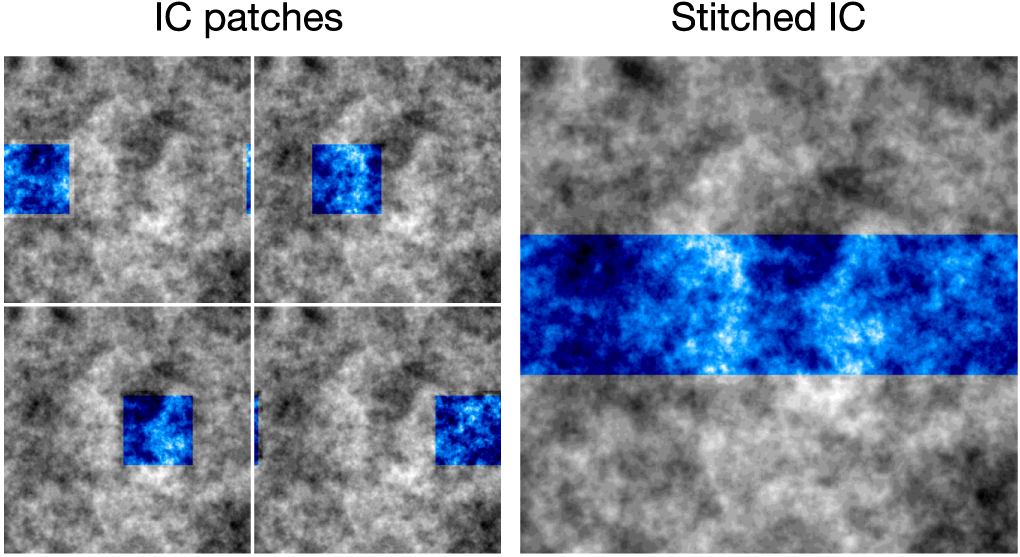
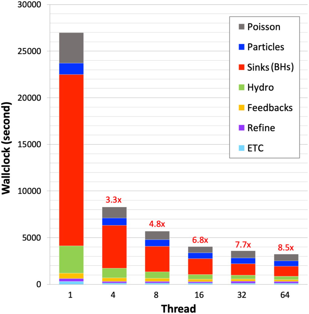
Figure 21. Cosmic variance presented in the two-point correlations measured from the gas (right) and dark matter (left) density fields at z = 200. Olive shades show the 1σ distribution of the two-point correlations in the 6400 subvolumes sampled from 100 ICs generated using different random seeds, and magenta curves indicate those in the whole volume of HR5 derived using the FFT. Black solid lines come from the linear theory. Red circles mark the measured correlations in the zoomed region of HR5. The two-point correlations in the zoomed region are situated within the 1σ scatter of the correlations of the subvolumes.
Download figure:
Standard image High-resolution image
Footnotes
- 13
- 14
- 15