


Abstract
This paper studies the energy dissipation of nonthermal electrons in the chromospheric flare ribbons during the peak time of a Geostationary Operational Environmental Satellite X-class flare (SOL2011-09-06) using desaturated Solar Dynamics Observatory/Atmospheric Imaging Assembly extreme-ultraviolet (EUV) narrow-band images. The temperature distribution in emission measure, called the differential emission measure (DEM), derived from the EUV fluxes from the flare ribbons shows an increase in the emission measure up to a temperature around 9 × 10⁶ K, followed by a steep decline at higher temperatures. In contrast, the flare loop reaches temperatures up to 27 × 106 K. This result is in agreement with previously reported single-temperature measurements using soft X-ray filter images, as well as DEM distributions reported for smaller flares obtained from EUV line observations. The main difference between small and large flares appears to be an increased emission measure in the flare ribbons, while the ribbon peak temperature is similar for all flares. This is different from the flare loop temperatures, where the hottest temperatures occur in the largest flares. However, the physically relevant quantity for energy dissipation, the energy content of the heated plasma as a function of temperature, does not need to peak at the same temperature as the DEM. The poorly constrained source thickness in radial extent of the flare ribbons has a significant impact on the shape of the differential thermal energy distribution. In particular, if the highest temperatures occur over a wide radial extent as "evaporating" plasma starts expending, the largest amount of energy could potentially be hidden above the peak temperature of the DEM.
Export citation and abstract BibTeX RIS
1. Introduction
Solar flares are powered by an impulsive release of magnetic energy in the solar corona. A significant part of the released energy goes into the acceleration of particles (e.g., Emslie et al. 2012). Due to the low particle density of the corona, flare-accelerated particles generally travel through the solar corona with negligible collisional energy losses. For particles entering the much denser chromosphere, however, collisional losses become the dominant energy loss mechanism, and flare-accelerated electrons produce bremsstrahlung emissions in the hard X-ray range and nuclear interactions of accelerated ions emit γ-ray emissions. The energy loss through hard X-ray and γ-ray emissions is minimal, but most of the collisional losses go into heating the chromosphere. As flare-accelerated electrons mainly penetrate the chromosphere at the footpoints of flare loop arcades, chromospheric heating creates so-called flare ribbons. Depending on the temperature of the flare ribbons, thermal emission from the ribbons is seen at various wavelengths from the infrared up to the X-ray range. Combined studies of the energy deposition derived from hard X-ray and γ-ray observations and the resulting thermal radiation from flare ribbons are therefore a key diagnostic to study energy dissipation in solar flares (e.g., Fletcher et al. 2011; Holman et al. 2011; Kontar et al. 2011).
The most detailed diagnostics of the energy input into flare ribbons from accelerated electrons are from hard X-ray observations taken by the Reuven Ramaty High Energy Solar Spectroscopic Imager (RHESSI; Lin et al. 2002; for review see Fletcher et al. 2011), and more recently also by hard X-ray focusing optics telescopes such as the Nuclear Spectroscopic Telescope Array (e.g., Glesener et al. 2020) and the Focusing Optics X-ray Solar Imager (e.g., Athiray et al. 2020). RHESSI also provided the first diagnostics of heating by flare-accelerated ions (Hurford et al. 2003, 2006), but observations in the γ-ray range are much more difficult to obtain compared to the hard X-ray range limiting the diagnostics of precipitating ions to only a few flares. The hard X-ray sources are generally observed to be elongated along the flare ribbons, but with an unresolved width (Dennis & Pernak 2009), and for events with the best statistics an upper limit of the hard X-ray ribbon width of 1.1'' has been reported (Krucker et al. 2011a). For such narrow ribbons, the energy input by flare-accelerated electrons is astonishingly high, making these beams no longer a dilute tail on top the ambient plasma distribution (Krucker et al. 2011a), and therefore poses a challenge to existing flare models.
The heating of flare ribbons is a complex interplay of the initial condition of the chromosphere, the energy deposition rate, ionization levels, and radiative and conductive losses. From an observational standpoint, heated plasma over a wide temperature range is observed. The densest of the heated layers are at or near the photosphere and are observed to slightly increase above the photospheric temperatures producing white light continuum emissions. Layers heated to higher temperatures are seen in UV lines and extreme-ultraviolet (EUV) lines. The hottest temperatures are seen in selected EUV lines and in the X-ray range. An overview of the different diagnostics tools in EUV and soft and hard X-rays is given in Figure 1.
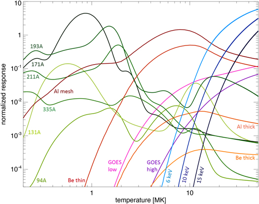
Figure 1. Overview of the thermal diagnostic tools in the EUV lines, soft X-rays, and hard X-rays used in this paper. The temperature response functions from various instruments at several wavelength bands are shown (as marked) assuming coronal abundances. The EUV filters are from the Solar Dynamics Observatory/Atmospheric Imaging Assembly (SDO/AIA), while the soft X-ray filters are from Hinode/XRT. In order to plot all curves in a single figure, the response functions are separately normalized for each instrument. The normalization between the different instruments is arbitrary.
Download figure:
Standard image High-resolution imageImpulsive soft X-ray emissions from flare ribbons have been investigated using observations from Yohkoh/X-ray Telescope (XRT; Tsuneta et al. 1991). McTiernan et al. (1993) and Hudson et al. (1994) independently reported impulsive emissions from a Geostationary Operational Environmental Satellite (GOES) M9.1 and GOES X1 flare, respectively, at temperatures of 9.6 and 9.8 ± 1.7 × 10⁶ K, while the coronal flare loop has significantly higher temperatures with values up to 25 × 106 K (McTiernan et al. 1993). The statistical study of Mrozek & Tomczak (2004) of more than 200 Yohkoh SXT flares confirmed that the temperatures of flaring ribbons are generally around 8.5 × 10⁶ K, with only a few events with temperatures up to 15 × 106 K. All these studies use the ratio of the Be119 and Al12 filter observations to estimate temperatures assuming that there is a single temperature dominating the emission. These two filters have a ratio that is monotonically increasing up to temperatures above 50 × 106 K providing therefore solid temperature diagnostics of plasmas of several millikelvins up to the hottest flare temperatures, as long as the single-temperature approach is justified. These Yohkoh results are therefore a strong indicator that flare ribbon emission measure (EM) distribution peaks around ∼10 × 106 K, and any higher temperature plasma from the flare ribbons therefore must be at significantly lower EMs in comparison. The impulsive soft X-ray peaks show a rapid rise (typically 30 s) and a decay that is only slightly slower (typically 40 s). The rise is generally correlated with the occurrence and duration of hard X-ray bursts. The statistical study of soft X-ray flare ribbons by Mrozek & Tomczak (2004) therefore strongly supports the standard picture that flare-accelerated electrons heat the flare ribbons, but the peak in the differential emission measure (DEM) of flare ribbons is at temperatures well below the temperatures seen in the coronal flare loops that can reach up to 50 × 106 K (e.g., Caspi et al. 2014).
As flare sources are likely multi-thermal, the single-temperature assumption used in filter-ratio measurements is a simplification that can introduce biases. It is therefore highly desirable to derive a DEM distribution by combined measurements at several EUV and soft X-ray wave bands (e.g., Fletcher et al. 2013), or even better, at several individual emission lines (e.g., Graham et al. 2013; Kennedy et al. 2013). Graham et al. (2013) reported a statistical study of microflares with GOES classes between B1 and C1 showing DEMs of flare ribbons that increase in temperature with a peak around 8 × 10⁶ K. At higher energies, the DEM strongly decreases, consistent with the soft X-ray results discussed above. The slope of the derived DEM is consistent with a scenario in which the deposited flare energy directly heats the top layer of the flare chromosphere, while deeper layers are heated by conduction.
For large flares, however, saturation of flare ribbons limits the diagnostics, in particular for SDO/AIA observations. With the newly available desaturation algorithm for AIA we can now overcome the saturation issues (Schwartz et al. 2014, 2015; Torre et al. 2015). The algorithm uses diffraction patterns produced by a set of meshes, which are used in the instrument design to hold filters. Under normal operation, the diffraction pattern is not visible, but during flares when the most intense sources saturate, the diffraction pattern becomes detectable up to high orders (e.g., Lin et al. 2001). From the diffraction patterns, however, the saturated part of the image can be reconstructed (for details we refer to Schwartz et al. 2014). The accuracy of the reconstructed fluxes is at 5% or better, as demonstrated in Torre et al. (2015) (see Table 2 of their paper).
This paper is an application of the desaturation algorithm for scientific exploitation. For a detailed description of the desaturation tool and it is viability we refer to previously published works (Schwartz et al. 2014, 2015; Torre et al. 2015). To simplify the analysis, we select an easy to desaturate flare with a high degree of saturation and clear diffraction patterns that occur at locations of low background emission. We first discuss the flare ribbon structure during the impulsive phase of flare images in the EUV range and hard X-rays. Then the DEM distribution is derived from the EUV data followed by a comparison of the obtained flare ribbon parameters with the coronal flare loop and the nonthermal energy input by flare-accelerated electrons as observed by RHESSI. The obtained results are discussed and compared to previous observations, and we highlight that the peak temperature in the DEM should not necessarily be interpreted as the temperature where most of the energy deposition occurs. Hotter layers at larger radial extents compared to the layer at peak temperature of the DEM can contain significant thermal flare energy, despite their small EM.
2. Observations
The flare (SOL2011-09-06) analyzed here is a GOES X2 flare that has been discussed in the literature for many different aspects from flare initiation through the interplanetary expansion of the associated coronal mass ejection (Dai et al. 2013; Feng et al. 2013; Kennedy et al. 2013; Liu et al. 2014; Xu et al. 2014; Yang et al. 2014; Dissauer et al. 2016; Janvier et al. 2016; Kawate et al. 2016; Kuhar et al. 2016; Macrae et al. 2018). The flare was selected for our single event study using the desaturation algorithm as it has one of the most intense flare ribbons and it was well observed in hard X-rays by RHESSI. Figure 2 shows the RHESSI hard X-ray images at the peak of the impulsive phase with the nonthermal emission seen from the two ribbons and a thermal loop connecting the ribbons. The nonthermal emission represented by blue 30–80 keV contours come from two well-separated and elongated flare ribbons. The thermal emission given by the magenta 5–12 keV contours connect the two ribbons, but the ribbons themselves are not seen in thermal emission (that the thermal flare loop covers the northern flare ribbon is due to projection effects, while indeed all thermal emission comes from the flare loops). The absence of thermal emission from flare ribbons is expected, and attributed to RHESSI's limited dynamic range in combination with the extreme difference in intensity of the ribbons relative to the loop emission in the hard X-ray range (see also discussion later in Section 2.4.1). In any case, this flare is a classic two-ribbon flare. As generally reported (e.g., Dennis & Pernak 2009), the hard X-ray ribbon is observed to be extended along the ribbon, but the ribbon width is not resolved by RHESSI.
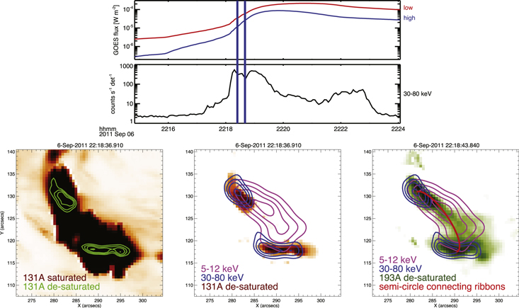
Figure 2. Overview of the AIA EUV and RHESSI hard X-ray observations during the impulsive phase of SOL2011-09-06T22:20 (X2.1). The top panel gives GOES and RHESSI X-ray flare light curves as time references for the images shown below, with the blue bars indicating the integration time of the RHESSI images. Imaging in the EUV range and hard X-rays shows the standard two-ribbon flare picture with flare ribbons seen in nonthermal hard X-rays and thermal EUV, while the coronal hot loop is seen in hard X-rays below ∼20 keV (contour levels shown are 30%, 50%, 70%, and 90% of the peak). (Bottom left) The saturated 131 Å image (dark corresponds to enhanced emission) is compared with the desaturated image, which is given in green contours. (Bottom center) The desaturated 131 Å map is displayed with RHESSI thermal (5–12 keV, magenta) and nonthermal (30–80 keV, blue) observations shown as contours. RHESSI maps are reconstructed using the CLEAN algorithm (Hurford et al. 2002) around the AIA 131 Å exposure time, but with an integration time of 16 s compared to 0.5 s for the 131 Å image. (Bottom right) The desaturated 193 Å image is show in the same format as the figure in the center. The desaturated 193 Å image reveals the flare ribbon as well as faint emission from coronal flare loop (see Section 2.4.1. for details). For reference, the red curve represents the projected position of a semicircle anchored with one end in each of the two ribbons standing normal to the solar surface.
Download figure:
Standard image High-resolution imageDue to the extreme brightness of the event, the SDO/AIA images from the ribbons are saturated, even for the images with automatic exposure control. These are the ideal conditions to apply the AIA desaturation algorithm developed by Schwartz et al. (2014). From our physical understanding of flares, we expect to see strong EUV signals from within the hard X-ray flare ribbons produced by the energy deposition of precipitating energetic electrons. Hence, we have a strong test for the desaturation algorithm. It must find the reconstructed EUV ribbons to coincide within nonthermal hard X-ray sources. Figure 2 shows an example of a saturated and desaturated image for the 131 Å wavelength band. The desaturation appears to work very well showing the same ribbon structure as seen in the hard X-ray range. From the desaturated images we estimate the flare ribbon lengths of 7'' and a rather narrow width of around 1''. The reconstructed 193 Å image with its hot response due to Fe xxiv at 192.03 Å shows in addition to the ribbons the coronal flare loops connecting the two flare ribbons (Figure 2, right). In the next section we present the DEM analysis from the desaturated ribbon fluxes using all six EUV channels from AIA, and then the derived flare ribbon parameters are compared to the values from the coronal loop given from the RHESSI hard X-ray data.
2.1. DEM from Flare Ribbons Derived from AIA
As this is the first time that have we derived the DEM from desaturated AIA fluxes, we simplify the task by only analyzing a single time during the impulsive phase of the flare with images taken between 22:18:36 and 22:18:48 UT. Relative to the main hard X-ray emission that starts at 22:18:05 UT and has at least five peaks until 22:19:00 UT followed by a decay of about a 30 s duration, the selected AIA images represent a time in the middle of the impulsive phase after electron precipitation has occurred for about 30 s (see Figure 2, top). To avoid potential uncertainties in the detailed shape of the reconstructed flare ribbons, we only derived DEM distribution from the total flux from each ribbon. The more challenging task of looking into details of the flare ribbon morphology and time evolution is left until the successful completion of the feature-averaged, single time step analysis presented here (see also discussion on timescales at the end of Section 2.5).
We use the regularized inversion code from Hannah & Kontar (2012) to derive separate DEM distributions for the northern and southern ribbons (Figure 3). To test the robustness of the code and test the possible influence of systematic errors of the desaturation code, we rerun the code with randomly added uncertainties of up to 20%. We note that the 20% uncertainty assumed here is a conservative assumption, as it is well above the 5% accuracy of the desaturation algorithm estimated by Torre et al. (2015). The results appear to be consistent showing a peak EM around 9 × 10⁶ K with a steep decline in EM at higher temperatures. At lower energies the EM is significantly reduced, by a factor of 20 around 2 × 10⁶ K, for example. There is a dip in the distribution around 4 × 10⁶ K, but it is unclear if the dip is a real feature or if it is due to the rather weak diagnostic ability of AIA at these temperatures (see Lemen et al. 2012, Figure 13). As the uncertainties are largest for those temperatures, the gap remains questionable. The derived peak temperature and peak DEM value agrees well with the full-disk DEM derived from SDO/EUV Variability Experiment (EVE) data for the same event (Kennedy et al. 2013, Figure 3(d)). There is also a hotter component in DEM derived from EVE data peaking between 20 and 25 × 106 K, which we attribute to the coronal emissions seen in hard X-rays and in Fe xxiv (see discussion in Section 2.4).

Figure 3. DEM results obtained from the desaturated EUV ribbon images. Results from the two ribbons are shown separately (top and center row), while the bottom row compares the combined ribbon results with the spectral fitting results from the hard X-ray coronal source. The first column shows the DEM with the red curves corresponding to the observed data and the black curves result from adding 20% random uncertainties to the data. The center row shows the expected GOES low-energy channel flux from the DEM shown to the left. The level of the GOES flux observed at the time when the EUV images were taken is shown as a dashed line. The right column gives the thermal energy content assuming a thickness of the ribbons of 1''. The fitting parameter of the coronal hard X-ray source is given in magenta in the bottom row.
Download figure:
Standard image High-resolution imageIgnoring the potential gap around 4 × 10⁶ K, the derived temperature distribution of the flare ribbons of this X-class flare looks similar to the DEM from a range of B class flares from Graham et al. (2013), except that the EM values are much higher. Graham et al. (2013) had peak temperatures around 8 × 10⁶ K and DEM values from 1028–1029 cm−5; here we report ∼9 × 10⁶ K and 2 × 1031 cm−5, respectively. Hence, the EM per area is enhanced roughly proportional to the difference in GOES class between the events considered, but the ribbon temperature is in the same range. This comparison indicates that the enhanced EUV flux in this X-class flare is due to a larger EM, i.e., due to an enhanced density and/or an enlarged volume of the flare ribbons. To estimate the density of the hot ribbon, we first sum the DEM over the hot component giving 1.9 and 2.5 × 1048 cm−3 for the northern and southern ribbon, respectively. The volume estimates are not well constrained by observations mainly because of the unknown radial extent of the flare ribbons in the EUV range, but also because of the ribbon width. Therefore, we use three different assumptions to estimate the ribbon volume and this consequently results in a range of densities. The ribbon length is 7'' for all assumptions. As a lower value for the ribbon thickness, we use a very narrow and thin ribbon of 0.3'', while for a large volume we assume a width of 1'' and a radial extend of 2''. To get a middle range for volume estimate, we use an equal width and radial extent of 1''. With these three assumptions, we get a middle value for the density of 9 × 1011 cm−3, and extreme values of 6 × 1011 cm−3 and 3 × 1012 cm−3, respectively. The densities derived here are above the values from the statistical study of soft X-ray flare ribbons by Mrozek & Tomczak (2004), which revealed densities up to 6 × 1011 cm−3 with most values below 2 × 1011 cm−3. However, the areas used for deriving their densities were taken from 10% contours of the soft X-ray images with a pixel size of 2.45'' and an FWHM angular resolution of 3.7''. Hence, an unresolved ribbon width results in a 10% width of around 8''. Assuming such a wide ribbon, the event discussed here would have a density within the statistical spread of the study of Mrozek & Tomczak (2004). Considering that more recent observations revealed narrow ribbon structures (e.g., Dennis & Pernak 2009), the volume estimates used in Mrozek & Tomczak (2004) are therefore upper limits, and densities are accordingly lower limits.
It is straightforward to derive the column density NEUV within the hot EUV source, and then the largest energy (in keV) of nonrelativistic electrons that completely stop within the EUV source can be estimated by (e.g., Emslie 1978):

For the different selected volumes, the values of Estop vary only slightly between 21 and 24 keV. Hence, electrons below these values seem to be able to stop within the EUV source, while higher energy electrons actually fly through the EUV source and precipitate toward deeper layers in the chromosphere, at least in the simplest propagation model. For electron transport in more complex models (such as collisional pitch angle scattering, mirroring, etc.), higher energy electrons could potentially also stop within the EUV source.
2.2. The GOES Soft X-Ray Flux from the EUV Ribbons
From the derived DEM, we calculate the expected GOES flux for each temperature bin (Figure 3, center column). The peak in the GOES flux distribution is slightly shifted in temperature to 10 × 106 K compared to the DEM temperature peak, but the bins with large DEM clearly produce the largest contribution. In total for both ribbons, we estimate a GOES flux in the low channel corresponding to a C5 GOES level. This is about 10% of the actual observed GOES flux at that time in the low-energy channel. Due to the low peak temperature of the flare ribbon DEM, the high-energy channel only increases by 1.5%. These estimates show that the flare ribbon can contribute to the GOES soft X-ray flux, in particular early in the impulsive phase, even though at a moderate level.
2.3. Thermal Energy Content Estimates
While the DEM distribution can be directly obtained from observations, the energy content as a function of temperature is the physically more relevant distribution. We estimate the thermal energy content using the standard formula (e.g., Hannah et al. 2011) assuming the same radial extent of the ribbon for all temperatures and neglecting radiative and conducting losses:

where T is the temperature, k the Boltzmann constant, EM(T) is in units of (cm−3), and V(T), A(T), and h(T) are the volume, area, and thickness of the ribbon, respectively. Assuming the same volume for all temperatures, the thermal energy distribution shows that most of the energy is around the peak temperature of the emission measure with a steep decline to a lower temperature. For the total EM of the hot component (see Table 1), using Equation (1), we get a total thermal energy content of 5.4 × 1028 erg assuming a volume of 7'' × 1'' × 1'' for each ribbon.
Table 1. Summary of the Parameters Derived from AIA, RHESSI, and GOES a
| Thot (106 K) | EMhot (1048 cm−3) | GOES Low b | GOES High b | Volume | n (1011 cm−3) | |
|---|---|---|---|---|---|---|
| Southern | 8.5 | 1.9 | 2 × 10⁻⁶ (C2) | 1 × 10⁻⁷ | 7'' × 1'' × 1'' | 8.4 |
| EUV ribbon | 7'' × 0.3'' × 0.3'' | 28 | ||||
| 7'' × 1'' × 2'' | 5.9 | |||||
| Northern | 9.0 | 2.5 | 3 × 10⁻⁶ (C3) | 2 × 10⁻⁷ | 7'' × 1'' × 1'' | 9.7 |
| EUV ribbon | 7'' × 0.3'' × 0.3'' | 32 | ||||
| 7'' × 1'' × 2'' | 6.9 | |||||
| Combined | 5 × 10⁻⁶ (C5) | 3 × 10⁷ | ||||
| EUV ribbon | ||||||
| Coronal | 26.8 ± 1.3 | 17 ± 3 | 5 × 10⁻⁵ (M5) | 5 × 10⁻⁵ | 24'' × 7'' × 5'' | 2.3 |
| hard X-ray loop | 24'' × 7'' × 10'' | 1.6 | ||||
| 24'' × 7'' × 1'' | 5.2 | |||||
| GOES | 23.6 | 21.2 | 5.4 × 10⁻⁵ (M5) | 2.3 × 10⁻⁵ | ||
Notes.
a GOES values are taken at 22:18:37 UT, while the hard X-ray and EUV parameters are averaged over a window of 16 and 12 s around 22:18:37 UT, respectively. b For the row labeled "GOES," the actual observed value of the GOES flux is given, while the other values are derived from the Te and EM of the EUV ribbon and hard X-ray loop, respectively.Download table as: ASCIITypeset image
The weakness of the above simple estimation of the thermal energy content is in the assumption of an equal volume for all temperatures. The temperature structure in the chromosphere is likely layered with an increasing temperature with altitude. For such a thickness distribution, the thermal energy distribution has a different shape as shown in Figure 3. As the layers at lower temperatures are expected to be thinner compared to the layers at high temperatures, the distribution of the thermal energy content would undergo an even steeper decline with decreasing temperatures than those shown in Figure 3. On the other hand, the hottest temperature could have larger radial extends h, in particular if "evaporation" of chromospheric plasma occurs and the high-temperature plasma is distributed over a large radial distance. In such a case, the peak temperature in the thermal energy content could be at a higher temperature as shown in Figure 3. As an example, we approximate how much thicker the 20 × 106 K plasma source needs to be compared to the 9 × 10⁶ K layer so that the 20 × 106 K plasma has the same energy content as the plasma at the peak temperature of around ∼9 × 10⁶ K. From Equation (2), we can see that the thermal energy scales linearly with temperature and it depends on the square root of DEM(T) × h(T). The derived DEM is about 15 times smaller at 20 × 106 K compared to the peak value (see Figure 3). Hence, to make the 20 × 106 K thermal energy content as high as the peak value in Figure 3 (i.e., a flat distribution), the spatial extent at 20 × 106 K would need to be about four times larger than at the peak temperature (∼9 × 10⁶ K). Such a value is potentially plausible in an evaporation scenario. In any case, it shows that the peak temperature in the DEM does not necessarily imply that the thermal energy content distribution peaks around the same temperature. It highlights that the unknown distribution of the altitude of heated plasma significantly limits our diagnostic capabilities for flare ribbons.
2.4. RHESSI Hard X-Ray Observations
In this section we derive from RHESSI hard X-ray observations the parameters of the hot coronal loop as well as for the nonthermal component to compare with the values derived for the ribbons. We use standard RHESSI imaging and spectroscopy techniques to derive the temperature, density, and thermal energy content of the main thermal flare loop using the time range over which the AIA images used in the DEM analysis are taken. The RHESSI spectral observations show the typical thermal and nonthermal components, with the thermal component being larger below 22 keV (Figure 4).
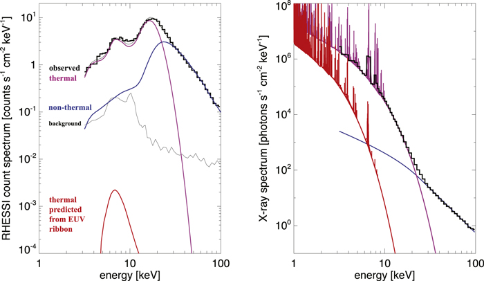
Figure 4. Hard X-ray spectral observations. (Left) RHESSI count spectrum fitted with the standard RHESSI software (using the CHIANTI atomic database (Dere et al. 1997) and coronal abundances) with a thermal (magenta) and nonthermal (blue, thick target fit, Brown 1971) component around the time of the EUV images shown in Figure 2. As both RHESSI attenuators have been inserted to handle the large count rates, the count spectrum peaks around 18 keV with the emissions at lower energies being heavily attenuated. The red curve gives the expected hard X-ray spectrum of the EUV-emitting flare ribbon. The thermal emission from the ribbons is well below the instrumental background emission (gray curve) and it is therefore not detectable by RHESSI. (Right) Photon spectrum derived from the observed count spectrum by removing the RHESSI instrumental response. The thermal spectra are shown in high spectral resolution to highlight the many spectral lines at lower energies.
Download figure:
Standard image High-resolution image2.4.1. Thermal
Around the hard X-ray peak time, a single thermal fit to the flare-integrated RHESSI spectrum gives a temperature of 26.9 ± 1.3 × 10⁶ K and EMHXR = 17 ± 3 × 1048 cm−3. As generally observed in large flares, the thermal fit dominates the flare-integrated spectrum below ∼15 M (see Figure 4, left). Because the 5–12 keV RHESSI image in Figure 2 shows the flare loops, the derived flare-integrated thermal parameters are essentially the temperature and EM of the flare loops. Hence, the coronal flare loops seen in hard X-rays (i.e., the hottest flare loops) are about three times as hot as the flare ribbons and has an EM that is roughly three times larger. In the next step, we test if the faint emissions in the AIA 193 Å passband seen in between the flare ribbons (Figure 2, right) are indeed from the same flare loops as the thermal hard X-ray emission detected by RHESSI. From the RHESSI thermal parameters of the flare loop we estimate that the hot response from Fe xxiv (192.03 Å) in the AIA 193 Å passband (Lemen et al. 2012) would produce a coronal loop with a flux of 3.8 × 10⁵ DN s−1 pixel−1. The observed fluxes integrated over the flare loop are (excluding the ribbons) in the desaturated 193 Å image shown in Figure 2 have a peak value of 5.2 × 10⁵ DN s−1 pixel−1, and averaged over the all pixels above 50% of the maximum value, we get 3.9 × 10⁵ DN s−1 pixel−1. The rather good agreement between the expected and derived fluxes strongly suggests that the coronal emission in the desaturated 193 Å images located in between the flare ribbons is indeed the hot flare loops as also seen by RHESSI (Figure 2, right). The GOES flux level derived from the RHESSI thermal source is M5, and roughly agrees with the observed GOES class at that time. This confirms that the GOES flux is indeed dominated by the hot thermal loop (see Section 2.2). Overall, observations of the thermal flare loop in the EUV range, soft X-rays, and hard X-rays give consistent results.
Figure 4 also shows the expected RHESSI count rate spectrum of the combined flare ribbon emission as derived from the desaturated AIA images (see Section 2.1). The predicated count spectrum shown in red is well below the instrumental background and also well below the low-energy tail of the nonthermal emission, indicating that RHESSI is far from being able to detect the thermal flare ribbon emission, at least for this flare. This is partially because the RHESSI attenuators have been inserted (A3 state) to handle the large count rates during this large flare. When the attenuators are inserted, RHESSI's low-energy response is greatly suppressed and the count rates at low energies are dominated by the off-diagonal response (i.e., the observed low-energy counts are from incoming photons at high energies). The photon spectrum shown on the right-hand side of Figure 4 shows the instrument-independent photon spectrum where the ratio of coronal loop to chromospheric ribbon is almost 104 at 10 keV, but only about 10 in the few kiloelectronvolt range. Hence, soft X-ray observations below the RHESSI energy range are better suited to simultaneously detect both the footpoints and the loop thermal sources (see Section 2.6) than the RHESSI hard X-ray observations.
To derive the density of the flare loop, we need to approximate the volume of the flare loop arcade. As the projection of a semicircle anchored on the two flare ribbons roughly traces the observed thermal hard X-ray source (see Figure 2, right), we use the semicircle length of ∼25'' and the ribbon lengths of ∼7'' as the two dimensions of the loop volume. The loop thickness is only poorly constrained by observations, and we therefore calculate the density for three thicknesses corresponding to 1'' (very thin sheet), 5'' (possibly the standard assumption), and 10'' (extended source) giving values of the density of 5.2 × 1011 cm−3, 2.3 × 1011 cm−3, and 1.6 × 1011 cm−3, respectively. Compared to the ribbon density, these values are about a factor of 3–4 lower. The derived thermal energy content of the flare loop at this time then becomes 116 × 1028, 82 × 1028, and 37 × 1028 erg, about 15 times larger than for the flare ribbons, at least under the assumption of a uniform radial source thickness.
2.4.2. Nonthermal
The main diagnostic power of the nonthermal part of the hard X-ray spectrum is to estimate the energy deposition rate by flare-accelerated electrons (e.g., Kontar et al. 2011). From the derived heating rate, it can be tested if enough energy is deposited to produce the hot EUV-emitting flare ribbons.
The high-energy (>22 keV) part of the hard X-ray spectrum shows a very strong nonthermal component with a rather hard spectrum (power-law indices up to 2.9 in the photon spectrum). The standard cold thick target assumption (e.g., Brown 1971) gives an energy deposition rate during the time of the EUV images of 6.2 × 1028 erg s−1 by electrons above 20 keV. As the limited dynamic range of RHESSI does not allow us to probe the nonthermal spectrum below 20 keV, a general problem of hard X-ray spectral observations (e.g., Kontar et al. 2011), the derived value is a lower limit. In any case, the energy deposition rate is large enough even if using the upper limit of 20 keV to heat the flare ribbons. The EUV ribbon that has a thermal energy content of 5.4 × 1028 erg could be heated within about ∼1 s. There are two main points that could complicate this simple consideration. A significant fraction of the energy in flare-accelerated electrons could be deposited at denser layers of the atmosphere below the ribbon structure at lower temperatures, and additionally, energy losses during the heating process could be important, as discussed in the next section.
2.5. Radiative and Conductive Losses of the Flare Ribbons
In this section, the radiative and conductive losses of the flare ribbons are approximated and then compared to the energy input by nonthermal electrons as derived from the hard X-ray spectral observations.
To estimate the radiative losses of the hot (>×106 K) ribbons we use the radiative emissivity curve η (i.e., total radiated power per unit of EM as a function of temperature for an optically thin plasma such as given in Figure 1 of Landi & Landini 1999):

where Thot and EMhot are the temperature and EM of the hot ribbon, respectively. With the values of temperature and EM derived in the previous sections (see Table 1), we get radiative losses of a few times 1026 erg s−1. As the EM of the colder plasma is declining faster than the radiative emissivity curve increases (see Figures 2 and 1 of Landi & Landini 1999), the radiative losses of the lower temperature EUV ribbon are smaller and they are not considered in our simple approximation. In any case, radiative losses of the hot ribbons are more than two orders of magnitude below the energy input for nonthermal electrons as derived above. Compared to the derived thermal energy content of the flare ribbon of 5.4 × 1028 erg, radiative cooling alone would take minutes to cool the flare ribbons after the energy input by flare-electron stop.
For the derived temperature and density of the flare ribbon, classic Spitzer conductivity is a valid approximation (see Figure 6 of Battaglia et al. 2009):

where κ0 = 106 erg s−1 cm−1 K7/2, Lz is the temperature scale length, and A is the total ribbon area. For T ∼ 9 × 10⁶ K, Lz = 1'', and A = 7.4 × 1016 cm2, we get a conductive loss rate of 2.2 × 1027 erg s−1. For shorter temperature scale lengths, the loss rate could be even larger. In any case, for all reasonable cases of Lz = 1'' conductive losses dominate over radiative losses, as is generally the case for flare ribbons (e.g., Fletcher et al. 2013; Simões et al. 2015). Integrated over the duration of the EUV emission, roughly 25 s from the start of the impulsive phase, conductive losses become of the same order of magnitude as the estimated thermal energy content. Hence, it is in principle not justified to neglect conductive losses when approximating the total thermal energy by simply taking the instantaneous thermal energy content (Equation (1)). Compared to the energy input by nonthermal electrons, however, conductive losses are about ∼30 times smaller than the energy input by electrons above 20 keV. Hence, as a rough approximation, conductive losses can be neglected for this event during the time of the main hard X-ray emission.
We finish this section by briefly discussing the timescales of the cooling of the flare ribbons and the required time resolution to properly measure ribbon cooling timescales. After the energy input by flare-accelerated electrons stops, conductive losses are able to cool the EUV ribbons rather efficiently with significant cooling on the timescale of the AIA image cadence of 12 s. The duration of the energy input by flare-accelerated electrons at a fixed location is limited not only by the duration of electron acceleration, but also because of the ribbon motion (e.g., Yang et al. 2009). As newly reconnected field lines make the flare ribbons move apart, the maximum duration of electron precipitation at a fixed location can be estimated from the ribbon width and the apparent ribbon velocity. For a ribbon width of 1'' and for a typical ribbon velocity of 30 km s−1, we get energy input at a fixed ribbon location of the duration of 24 s. This demonstrates the need for high time cadence EUV imaging observations below the available 12 s cadence provided by SDO/AIA. High cadence IR observations of flare ribbon heating and cooling reveals impulsive heating on a ∼4 s timescale, and exponential decay time of ∼10 s for a single event with well-separated individual hard X-ray peaks (Penn et al. 2016). Hence, a cadence of a few seconds is a minimum requirement to study heating and cooling of flare ribbons.
2.6. Soft X-Ray Imaging Observations
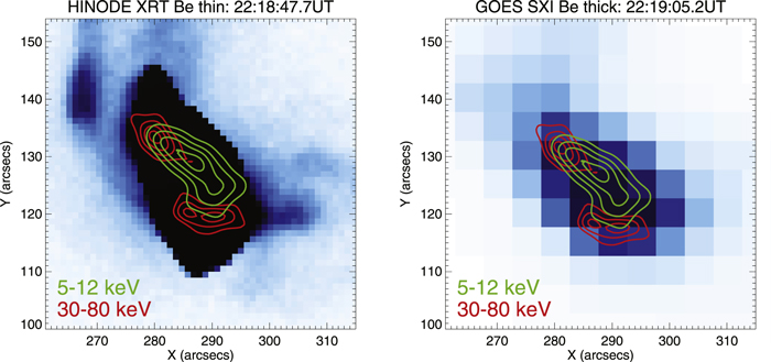
As discussed in Section 2.4.1, the best chance of simultaneously observing the thermal emissions from the ribbons and the loop is in the soft X-ray range. Figure 4 shows the extrapolation of the X-ray spectrum of the ribbon and loop thermal emissions down to 1 keV. While it is very challenging to simultaneously observe both thermal components in the hard X-ray range, it becomes easier at soft X-ray wavelengths as the difference in flux levels are becoming smaller. This can be seen in the derived GOES fluxes where the ribbons are about 10% in the low GOES channel signal, but down to 1.5% in the high channel (see Table 1). For soft X-ray filter observations the intensities of loop and footpoint sources can even be similar. For SOL2011-09-06, Hinode/XRT (Golub et al. 2007) provides a "Be-thin" filter image taken during the same time interval as the AIA images used in the derivation of the DEM shown in Figure 3. Using the derived EM and temperature pairs from AIA and RHESSI, we estimate a ratio of the ribbon to loop thermal component in the Be-thin image of 1.1 (for the XRT response function see Figure 7 in Golub et al. 2007). Despite the very low exposure time, the Be-thin image is unfortunately saturated (Figure 5). Nevertheless, the saturation signatures suggest emissions from the two flare ribbons as well as from the loop, as expected from our simple considerations given above. The only other soft X-ray images available for this time range are from the GOES Solar X-Ray Imager (SXI; Hill et al. 2005), but the image with the best temporal match is taken ∼20 s later when the GOES emission is already increased by more than a factor of 2. This SXI image is taken with the "Be 50 μm" (i.e., a thick Be filter), where low temperature emission is slightly more suppressed relative to high temperatures than for the Be-thin filter used by XRT. The expected ratio of the ribbon to loop thermal component is therefore about 0.5 (for response curves see Figure 11 of Pizzo et al. 2005). The SXI observations show indeed the coronal loop as the stronger source, but this could also be due to the later time of the SXI image when the thermal loop is much brighter as indicated by GOES and RHESSI. In summary, the available soft X-ray observations provide an unfortunately limited additional diagnostic power for this event.
Figure 5. Soft X-ray filter images from Hinode and GOES/SXI with the RHESSI contours from Figure 2 overplotted for reference. (Left) Hinode XRT thin-Be filter image taken during the same time interval for which the DEM shown in Figure 3 has been derived. Despite the short exposure time (0.008 s), the emission from the main flare location is saturated. Nevertheless, the saturation signal suggests that both ribbons as well as the coronal source are contributing to saturation. (Right) GOES SXI image taken 17 s after the XRT images. Saturation also occurs in this image, but only for the brightest pixels from the coronal source. The coronal source is strongest in this later image (see the text for details).
Download figure:
Standard image High-resolution image
3. Summary and Discussion
We used the desaturation algorithm by Schwartz et al. (2014) to reconstruct saturated AIA EUV emission from the ribbons of an X-class flare. With the reconstructed AIA fluxes we derived the DEM distribution of the ribbons and compared them to the main flare loop seen in hard X-rays. The results are summarized in Table 1. We found that the DEM of the flare ribbon peaks around 9 × 10⁶ K, while the main flare loop is at a much higher temperature around 27 × 106 K. These results are in agreement with earlier soft X-ray observations (McTiernan et al. 1993; Hudson et al. 1994; Mrozek & Tomczak 2004) that report ribbon temperatures around 10 × 106 K using a single-temperature approximation (filter-ratio method). The DEM of the flare ribbons of this large flare looks surprisingly similar to previously reported flare ribbon DEM distributions of much smaller flares (Graham et al. 2013). The main difference between small and large flares appears to be the much higher EMs for the X-class flare, but the distributions peak roughly around the same temperature.
The interpretation of the peak temperature in the DEM, however, is not straightforward. We cannot simply conclude that most of the energy content in the flare plasma is at the same temperature as the peak in the DEM curve. This is because the poorly constrained thicknesses of the different temperature layers have a significant influence on the thermal energy content as a function of temperature (see Equation (2)). Only for a uniform ribbon thickness, the energy content distribution would also peak around the same temperature as the DEM distribution. However, this is unlikely the case in flare ribbons. The values of the thermal energy content derived assuming a constant thickness, such as present in this work, are therefore only lower limits, since the thicknesses are expected to be increase with increasing temperature.
To further illustrate the importance of the poorly constrained ribbon volume, we discuss here briefly the EM definition. EM is most generally approximated by n2 V, where n is the density and V the volume of the radiating source, but it also can be written as N2 V−1, where N is the number of particles within the radiating source. For the same number of particles N (i.e., same energy content of the radiating plasma), an extended source has therefore a lower emission measure than a compact source. Hence, an extended source at equal energy content radiates much less brightly than a compact one. A temperature-dependent source volume consequently influences the shape of the DEM. It is therefore difficult to observe the hottest plasma in flare ribbons as it "evaporates" and spreads out over a larger volume. Hence, hottest particles are expected to create a dimmer EUV signal than the same number of particles seen in compact, cooler sources within the flare ribbon. Therefore, the turnover seen at higher temperatures in the DEM could be produced by a larger thickness of the hottest temperature layer, and not because of decreased heating at higher temperatures. Similarly, the filter-ratio method applied for flare ribbons has an intrinsic bias toward compact sources, and the derived thermal energy content is therefore a lower limit. As demonstrated in Section 2.3, this effect is likely significant for flare ribbons, as they have a complex and dynamic spatial and temporal response to heating by flare-accelerated electrons.
We encourage modelers to investigate the thickness of flare ribbon structures using simulations. In such a way temperature distribution of the hottest plasma could hopefully be better described. To resolve the actual thicknesses of individual temperature layers is very challenging, if not impossible. For limb observations where the radial extent could be in principle measured with high enough angular resolution, the EUV radiation cannot escape as the emission is absorb along the line of sight. Hence, the best chances are possibly events seen partially from the side with very high angular resolution provided by future telescopes.
The derived density of the flare ribbons is not that well constrained by observations because of the not well-known source volume. We estimate most likely values of ∼9 × 1011 cm−3 with extreme values being a factor of ∼2 smaller or up to a factor of ∼3 higher. The column density to stop flare-accelerated electrons, however, is much better constrained suggesting that electrons below 20 keV are stopped within the EUV ribbon, but higher energy electrons can actually fly through the EUV source and penetrate deeper, at least in the simplest transport models. This suggests that the EUV ribbon source is heated by the low-energy tail of the flare-accelerated electrons. This is consistent with the picture brought forward by Kuhar et al. (2016), where the high-energy electrons above ∼30 keV are responsible for the white light flare production, while the low-energy end is speculated to heat the upper part of the chromosphere. However, in our study we only look at a 20 s averaged snapshot of a highly dynamic flare evolution, which indicates that this interpretation is a very simplified view. Furthermore, for transport models including collisional pitch angle scattering or magnetic mirroring, the stopping column density could be increased and also higher energy electrons could potentially stop within the EUV source.
3.1. Outlook
The next step in our AIA flare ribbon study will be to look at other events to corroborate that the DEM generally peaks around 10 × 106 K for all flares. Furthermore, the diagnostics of the AIA diffraction patterns are not limited to reconstructing the saturated images as used in this paper, but the wavelength dependence of the diffraction acts as a spectrometer. The diffraction patterns show a convolution of the source shape and the source spectrum within the EUV passband. The high-order patterns can therefore be used to extract spectral information of the saturated sources (e.g., Krucker et al. 2011b). Such analyses are planned to be carry out for AIA data as well, but the topic is proving to be challenging (Raftery et al. 2011).
Soft X-ray and spectral EUV observations from HINODE are excellent diagnostics to better limit the steep decline of the high-temperature component in flare ribbon DEM distributions. Saturation of these instruments during the biggest flare in combination with the slit position being located on the flare ribbons, however, makes such observations rather rare. The heavily underused HINODE/EIS slot images (Harra et al. 2020) are a further excellent diagnostic source that should be added to improve our understanding of flare ribbon temperature distributions. Optical observations should be used in the future to constrain the coolest heated layers within the flare ribbons, in particular with the Daniel K. Inouye Solar Telescope (e.g., Tritschler et al. 2016).
To detect flare ribbons in hard X-rays is very challenging for indirect imaging such as RHESSI or the Spectrometer Telescope for Imaging X-rays onboard the Solar Orbiter (Krucker et al. 2020). The sensitivity and imaging dynamic range of these instruments is insufficient, in particular when attenuators are inserted during large flares. For the discussed X-class flare, the thermal emission from the flare ribbon is expected to be even lower than the extrapolated nonthermal emission for energies down to 7 keV. Hence, in hard X-rays, the low-energy tail of the nonthermal emission appears to be easier to detect than the thermal emission from the ribbons. For future observations with hard X-ray focusing optics (e.g., Krucker et al. 2014) with a much improved dynamic range in imaging and enhanced sensitivity, we will be able to detect X-rays from ribbons both in the thermal and nonthermal range providing direct diagnostics of both components.
Finally, we encourage modelers to use the derived parameters of energy input by electron beams from this flare, and see which conditions can reproduce the parameters for the flare ribbons.
We thank the anonymous referee for many detailed and insightful comments. The work was supported by NASA contract NAS 5-98033 for RHESSI and NASA grant NNX14AG06G. We thank A. Chavier for carefully reading our paper.