


Abstract
We present the reheating constraints on an inflationary universe induced by perfect fluid models. Starting with the descriptions for the observables of the scalar field inflationary models in the reconstructed methods, we outline the procedure of perfect fluid inflationary models through these methods to calculate the inflationary observables and reheating. We show that the reheating e-folds number Nre and the reheating final temperature Tre are bound depending on the finite range of reasonable values of  . By restricting the equation-of-state parameter in the reheating stage,
  , more stringent constraints can be derived for the model's parameter space of perfect fluid. These constraints correspond to viable values of the scalar spectral index ns and tensor-to-scalar ratio r, released by Planck2018 observational data.
Export citation and abstract BibTeX RIS
1. Introduction
The perfect fluid is an appropriate candidate for the universe that justifies the inflationary phase in the early universe; it has thus received much attention. Many scalar field inflationary models have been explored and constructed using several methods leading to the theoretical consequences compatible with the observational data obtained from Planck in terms of inflationary observables (Bamba et al. 2014c; Elizalde et al. 2014; Gao & Gong 2014; Hazra et al. 2014; Inagaki et al. 2014; Joergensen et al. 2014; Kobayashi & Seto 2014; Wan et al. 2014; Bamba & Odintsov 2016). The inflationary observables, the scalar spectral index ns, the tensor-to-scalar ratio r, and the running of the spectral index αs, in an ordinary scalar field model of inflation, are represented by using the potential of the scalar field. The spectrum of the density perturbations generated during inflation influences the potential form of the inflation (Linde 1982; Yokoyama & Maeda 1988; Freese et al. 1990; Lidsey et al. 1997). Perfect fluid models provided by the reconstructed scalar field models lead to information on the properties of the fluid models, accounting for the observables in the early universe. From a cosmological point of view, the consequences of this approach, which have been checked by using observations of the CMB, require novel conditions for the perfect fluid to be a viable theory. The fluid description of the universe has been used widely in both standard cosmology and inflation. Chaplygin gas and viscous fluid are two imperfect fluid models that attracted attention as a means of unifying inflation with dark energy (Bento et al. 2002; Bilić et al. 2002; Capozziello et al. 2006; Elizalde & Silva 2017). Descriptions of inflation were reconstructed in perfect fluid models in Bamba et al. (2014c, 2014d) and Bamba & Odintsov (2016). They re-expressed the observables of inflationary models, the spectral index of curvature perturbations ns, the tensor-to-scalar ratio r, and the running of the spectral index αs, in terms of the slow-roll parameters  and η in a fluid framework. Then, they analyzed fluid observables with the most recent Planck data (Bamba et al. 2014a, 2014b; Lahanas & Tamvakis 2014; Takeda & Watanabe 2014). In this work, we review two perfect fluid inflationary models that have different squares of the Hubble parameter. First, we investigate the evolution of inflationary parameters in each model to find suitable ranges for the energy density ρ, e-folds number N, and the constant coefficients of models. Then, we explore the reheating epoch of these two models. The acceptable ranges of inflationary parameters help us to earn precise constraints on the reheating e-folds number Nre and reheating final temperature Tre. Reheating is an effective mechanism to realize the hot Big Bang universe after the inflationary epoch that converts the energy of an inflation field to thermal radiation and includes the physics of particle creation and nonequilibrium phenomena. The reheating epochs have been explored on some inflationary models with a single scalar field that is specified by the potential energy density (Dai et al. 2014; Amin et al. 2015; Cai et al. 2015; Cook et al. 2015; Munoz & Kamionkowski 2015; Ueno & Yamamoto 2016; Lozanov 2019). We look for additional constraints, which arise from the reheating phase, on the inflationary parameters of the perfect fluid universe. If a fluid component with the cosmic equation-of-state (EOS) parameter ωre during the reheating era, dominates the energy density of the universe, the bounding on the reheating e-folds number and the reheating temperature will depend on ωre. Here we show that the reheating process may provide additional constraints to these inflationary perfect fluid models, which is modeled by an effective EOS parameter ωre. This paper is organized as follows. In Section 2 we introduce an inflationary universe with a perfect fluid component. We present the fluid inflation observables by conversion from the inflationary universe induced by a scalar field to the perfect fluid formalism. In Section 3 we present two descriptions of perfect fluid, linear, and exponential forms, respectively. There is a schematic comparison between parameter spaces of (r − ns) and (αs − ns) of perfect fluid models and Planck2018 data. Then, we show the evolution of , which reveals the intervals of constant coefficients in each model and helps us to provide more precise constraints in the next section. In Section 4 we introduce the description of the reheating phase with reheating e-folds number Nre and reheating final temperature Tre in terms of bounded EOS parameter ωre. Then we show the reheating constraints through a few graphs. In Section 5 we conclude the paper with a short discussion.
2. Inflationary Universe with Perfect Fluid Formalism
The action of an inflationary model with a single scalar field ϕ coupled minimally with gravity

where R is the scalar curvature, leads to the definition of slow-roll parameters.
2.1. Slow-roll Parameters
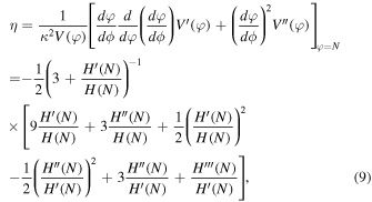
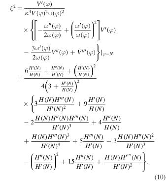
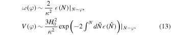
The definition of slow-roll parameters , η, ξ in terms of potential V(ϕ) are as follows
The prime denotes the derivative with respect to the argument of the functions such as  , etc. The expressions of the scalar spectral index ns of the curvature perturbations, the tensor-to-scalar ratio r of the density perturbations, and the running of the spectral index αs , for a single scalar field model are obtained as follow

There is increasing interest in constructing a scalar field inflationary model to determine the number of e-folds N, the slow-roll parameter , or the tensor-to-scalar ratio r by the observables (Lyth & Riotto 1999; Nojiri & Odintsov 2006). We assume the flat Friedmann–Lemaitre–Robertson–Walker (FLRW) metric

where the Hubble parameter is defined as  , and a(t) is the scale factor. The dot shows the time t derivative. The gravitational field equations in the chosen background are given by

In Bamba et al. (2014c, 2014d) and Bamba & Odintsov (2016), the scalar field inflation model was reconstructed to an inflationary universe with perfect fluid component. By redefining a new scalar field φ, which is identical to the number of e-folds N so that ϕ = ϕ (φ), the field equations can be rewritten as follows
In these reconstructed equations we consider  , and if the Hubble expansion rate H is a function of N, H(N), we can express ω (φ) and V(ϕ (φ)) in the following form
As a solution for the field equation ϕ or φ, we have H = H(N) and φ = N and it is explicit that H' < 0 (because ω (φ) > 0). Now we can write the slow-roll parameters , η, and ξ in terms of H
and
We can solve the slow-roll parameters with respect to H(N), but it is not so straightforward in (8)–(10). It is possible to recover the corresponding scalar field theory by using (7). In this reconstructed model, we explore the case that has the following condition

In this case, we achieve
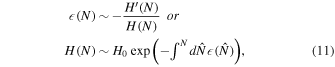
where H0 is a constant. The other slow-roll parameters have also become as follows
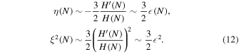
Then, by using Equation (8), we can obtain
After combining Equations (3), (11) and (12), we can find the observable parameters in terms of the slow-roll parameter as ns − 1 ∼ − 3, and αs ∼ − 32. So, an appropriate definition of H(N) in an inflationary model can link the reconstructed model and the scalar field theory.
2.2. Perfect Fluid Setup
To obtain the slow-roll parameters according to perfect fluid, we consider the gravitational field equations of fluid in the FLRW spacetime

where ρ is the energy density of the perfect fluid.

P is the pressure of the perfect fluid. We assume an arbitrary function f(ρ) (in terms of the energy density of the perfect fluid), and a rather general EOS parameter as follows

With this assumption, Equation (15) takes the following form

By using the conservation law, we obtain ρ' = − 3f(ρ). If we substitute it in Equation (17), a new relation is provided

Prime operating means the derivative with respect to the energy density of the perfect fluid  , whereas
  and
and  . Then we can rewrite the slow-roll parameters in terms of ρ (N) and f(ρ (N)).
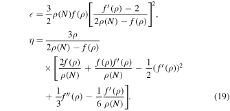
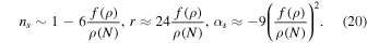
The observables for the inflationary model of perfect fluid, ns, r, and αs expressed in (3). These relations in terms of ρ and f(ρ), become new forms (Bamba et al. 2014d). If ρ and f(ρ) are affected by a very slow condition in the inflationary era as  , the relations in (3) are reduced to a simple form as
3. Reconstruction and Inflationary Descriptions of Perfect Fluid Models
We endeavor by testing two different examples for the square of the Hubble parameter to find the credibility of the reconstructed model for the perfect fluid. First, we examine the linear form and then the exponential form of the square of the Hubble parameter.
3.1. Linear Form
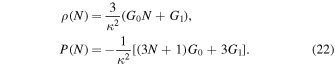
First, we examine the linear form for H2

where G0(<0) and G1(>0) are constants. The scale factor for the slow-roll exponential inflation is given by  (
( is a constant) in which Hinf is the Hubble parameter at the inflationary stage. In this stage, the Hubble parameter is approximately constant, so that its time dependence is weak. This weak time dependence of H is considered in Equation (21), in which the number of e-folds N, is assumed to play the role of time. During inflation, if we have
  , then the time dependence of the Hubble parameter is negligible. By using the gravitational fields equations for the perfect fluid in Equations (14) and (15) with Equation (21)) and H > 0, we obtain
After omitting N from these equations, and from Equation (21)) we obtain  . Therefore, by combining Equations (16) and (22), we acquire the EOS parameter as
The slow-roll parameters, along with the slow-roll conditions, help us to determine the logical values of the constants parameters of the linear perfect fluid inflationary model. The slow-roll parameters and η in terms of the energy density and the e-folds number in this model defined as

and

We expect the perfect fluid inflation obtained by a reconstructed formalism from the scalar field inflationary model gives rise to realizing inflation compatible with Planck2018 data. In this regard, we must first be able to determine the limits of the fixed parameters of Equation (21), G0 and G1. By using the slow-roll conditions, ≪ 1 and ∣η∣ ≪ 1, the amount of energy density ρ, the number of e-folds N and G parameters, at the end of the inflationary era is explicitly indicated in Figure 1, which are summarized in Table 1. In this case, the energy density at the end of the inflationary era is approximately equal to 1.44 GeV, which is necessary for our calculations in the reheating epoch in the next section. To check the acceptability of our perfect fluid inflationary model, we compare the model's observables with Planck2018 observational data. We have plotted r versus ns for the linear perfect fluid inflationary model in the background of Planck2018 data and performed some numerical analysis on the tensor-to-scalar ratio and the scalar spectral index as acquired in Figure 2. The blue rods in this figure, show the available ranges of (r − ns) for various values of G parameters in the allowed interval  . These results in the linear perfect fluid model seem to be near the results of the scalar field models with (V ∝ ϕn) potential for (
 ), between (50–70) e-folds, which are illustrated in Akrami et al. (2020b). Likewise, the rods in the interval
  , show some behavior similar to the power-law inflation. G parameters in this model can be related to the conventional scalar field models, through the expressions in (11) and (13). Additionally, we compare the running of scalar spectral index αs in this linear model with Planck2018 data. In this plot, we adopted
  , from the allowed range for the linear model in Table 1. We can see that the linear perfect fluid inflationary model is consistent with Planck2018 observation data, at least in some subspaces of the model parameter space.

Figure 1. (a) The evolution of with respect to  and N; (b) the evolution of , with respect to G0 and ρ, in the linear perfect fluid model.
Download figure:
Standard image High-resolution image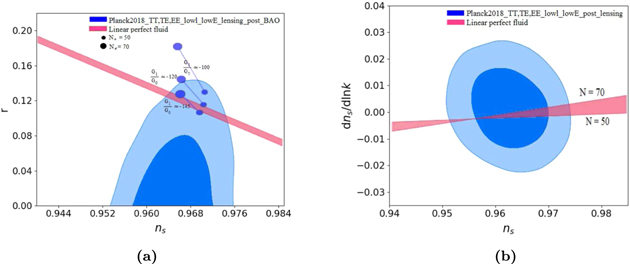
Figure 2. (a) The tensor-to-scalar ratio vs. the scalar spectral index; (b) the running of scalar spectral index vs. the scalar spectral index, in the background of Planck2018 data, for the specific linear perfect fluid model.
Download figure:
Standard image High-resolution image
Figure 3. (a) The evolution of , with respect to  and N, (b) the evolution of , with respect to G3 and ρ, in the exponential form of the perfect fluid model with β = 0.001.
Download figure:
Standard image High-resolution imageTable 1. The Acceptable Ranges of the Constant Parameters G0 and G1, As Well As the Admissible Intervals of the Energy Density ρ, and the Number of e-folds N, in the Linear Perfect Fluid Model
| G0 | ρ (GeV) |

|
N | ||
|---|---|---|---|---|---|
| Linear form of perfect fluid | −0.6 ≲ G0 ≲ 0 | 1.44 ≲ ρ ≲ 1019 |

|
65 ≲ N ≲ 80 |
Download table as: ASCIITypeset image
3.2. Exponential Form
In this case, we study the following exponential form for H2

where G2 (<0), G3(>0), and β (>0) are constants. There is also a motivation that convinces us to choose the exponential form of the perfect fluid inflationary model. The scale factor in the power-law inflation is expressed as  , where p is a constant. The square of the Hubble parameter during inflation becomes
 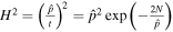 , which is equivalent to the form in Equation (26) with
  ,
,  , and G3 = 0. Therefore, this exponential form can describe the power-law inflation for the perfect fluid. By using the gravitational fields equations for the perfect fluid, Equations (14) and (15), with Equation (26) and H > 0, we obtain
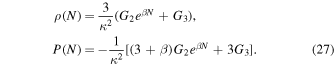
By eliminating N from these equations, we can obtain P(N) in terms of ρ (N)

By using Equation (27) and comparing Equation (28) with Equation (16), we obtain

So the EOS parameter, in this case, is as follows
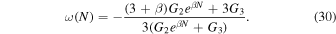
The slow-roll parameter and η, in terms of the energy density and the e-folds number in the exponential form of the perfect fluid inflationary model, defined as
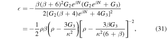
and
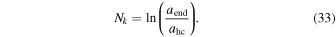
As in the previous case, we perform an investigation to determine acceptable intervals for the constant parameters G2 and G3 in this exponential form. Of course, it must be determined what space of other parameters, ρ and N, can produce standard inflation in this perfect fluid model. These goals are achieved by applying slow-roll conditions that are evaluated in Figures 3 and 4 for β = 0.001 and β = 0.01. The results of these evaluations are summarized in Table 2. In this case, the energy density at the end of the inflationary era for β = 0.001 and β = 0.01 is approximately equal to 2.85 and 0.45 GeV, respectively, which is necessary for our calculations in the reheating epoch in the next section. For values more or less than the values we have considered for the β parameter, we could not have acceptable results for the model. To test the viability of our exponentially perfect fluid inflationary model, we compare the model's observables with Planck2018 observational data. We have plotted r versus ns in the background of Planck2018 data and performed some numerical analysis on the tensor-to-scalar ratio and the scalar spectral index as acquired in Figure 5. There is a set of plots in acceptable ranges of G parameters that are illustrated by green rods in Figure 5(a). When we adopt  , the rods are placed in limits similar to the scalar field models with V(ϕ) ∝ ϕn, for (
 ) between 50 and 70 e-folds. The same scenario happens for the exponential perfect fluid model with β = 0.01. The plots in Figure 5(b) reveal a wide range of r − ns for
  which is compatible with Planck2018 data. There is also a comparison between the running of the scalar spectral index of the exponential perfect fluid model and the Planck2018 data. We have adopted values for G2 and G3 from the interval in Table 2. We see that these exponential perfect fluid inflationary models are consistent with Planck2018 data at least in some subspaces of the model parameter space.
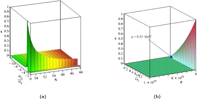
Figure 4. (a) The evolution of , with respect to  and N; (b) the evolution of , with respect to G3 and ρ, in the exponential form of the perfect fluid model with β = 0.01.
Download figure:
Standard image High-resolution image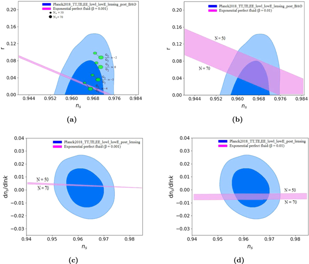
Figure 5. (a) Tensor-to-scalar ratio vs. the scalar spectral index for β = 0.001 and (b) β = 0.01, in the background of Planck2018 data, for the specific exponential perfect fluid model. (c) The running of the scalar spectral index vs. the scalar spectral index for β = 0.001 and (d) β = 0.01, in the background of Planck2018 data, for the specific exponential perfect fluid model.
Download figure:
Standard image High-resolution imageTable 2. The Acceptable Ranges of the Constant Parameters G2 and G3, As Well As the Admissible Intervals of the Energy Density ρ, and the Number of e-folds N, in Exponential Form of the Perfect Fluid Model
| G3 | ρ (GeV) |

|
N | ||
|---|---|---|---|---|---|
| Exponential form of the perfect fluid with β = 0.001 | 0 ≲ G3 ≲ 1200 | 2.85 ≲ ρ ≲ 1019 |

|
50 ≲ N ≲ 58 | |
| Exponential form of the perfect fluid with β = 0.01 | 0 ≲ G3 ≲ 19 | 0.45 ≲ ρ ≲ 1019 |

|
44 ≲ N ≲ 55 |
Download table as: ASCIITypeset image
4. Reheating after the Inflationary Universe with Perfect Fluid
Reheating is a necessary stage after inflation that transforms the energy stored in the inflation into a plasma of relativistic particles and to the thermal bath at the reheating temperature. The reheating stage is modeled by an effective EOS parameter  , a number of e-folds Nre, and a thermalization temperature Tre, (Dai et al. 2014; Amin et al. 2015; Cai et al. 2015; Cook et al. 2015; Munoz & Kamionkowski 2015; Ueno & Yamamoto 2016; Lozanov 2019). In the following, we tend to express the reheating parameters Nre and Tre in terms of the scalar spectral index. The relation between the number of e-folds and the scale factors ahc and aend, at the horizon crossing and the end of inflation, respectively, is given by
During the reheating era, the EOS parameter ωre, is supposed to be constant and any changes in the scale factor lead to significant changes in energy density. The relation between the energy density ρ ∼ a−3(1+ω), during the reheating era and the scale factor
where the subscript end refers to the end of inflation, and re refers to the reheating stage. ωre is the effective EOS parameter during the reheating era. The number of e-folds during the reheating in terms of the energy density and the EOS parameter in this era is as follows
If khc is the value of k when the modes exited the horizon, which is related to the present time, we get
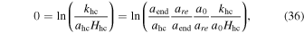
where 0 indicates the present time values and subscripts end and re, refer to the end of inflation and reheating era, respectively. We consider the pivot scale value k = 0.05 Mpc−1, at which Planck determines the scalar spectral index, and the parameters with this subscript are calculated at the time of horizon crossing (Aghanim et al. 2020; Akrami et al. 2020a). Combining the Equations (33)–(36), gives the following relation
The energy density in terms of the final temperature of reheating, is defined as

where gre is the effective number of relativistic species. The entropy conservation gives the relationship between the reheating entropy, which is preserved in the CMB, and today's neutrino background as:
 is the number of species for entropy at the reheating. The present temperature T0 of the CMB is approximately near to T0 = 2.725 K, and the current neutrino temperature is equal to
  . The relation between reheating temperature and the present CMB temperature by taking into account the entropy conservation is as follow
By rewriting this equation, we obtain
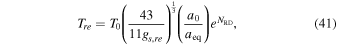
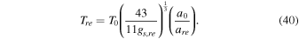
where NRD is the number of e-folds of radiation dominance  . By combining Equations (38) and (40), we reach the following relation
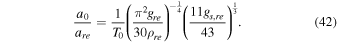
The ratio of a0/aeq could be the following form
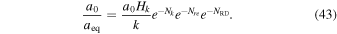
From the Equations (41) and (43), we achieve

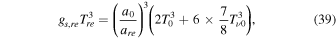
By making small changes in Equation (35), we can acquire the energy density of the reheating stage

The Equations (45) and (42) help us to obtain
By using the slow-roll approximation and the amplitude of the scalar perturbations, we can write

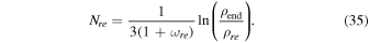
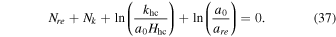
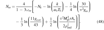
Finally by inserting Equations (37), (46), and (47), we compute the reheating number of e-folds expression
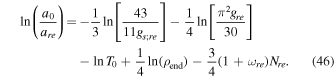
We adopt the amplitude of the scalar perturbation at the pivot wavenumber k = 0.05 Mpc−1 given by 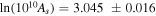 . The reheating final temperature in terms of the EOS parameter acquires from Equations (38) and (45)
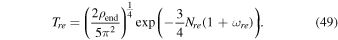
To reveal the reheating era for the reconstructed perfect fluid model that is mentioned in Sections (2) and (3), we are going to plot the number of e-folds Nre and the final temperature of reheating stage Tre, versus the scalar spectral index ns for various values of EOS parameter  . It is necessary to rewrite Equations (48) and (49) in terms of ns, and the final energy density ρend in the models is introduced by several plots in Figures 1, 3, and 4. In our computations, we have set c = 1,
  , Mpl = 1.2 × 10¹⁹ GeV. The e-folds number during reheating era has logarithmic dependence on , gre and
  , i.e., these parameters are not so effective in our calculations. The inflation era ends when the EOS parameter equals
  and the radiation era begins when this parameter equals
  . Supposing a massive inflation, immediately the EOS parameter rises to 0, the EOS of a massive harmonic oscillator oscillating between potential dominance and kinetic dominance (EOS of –1 and 1, respectively). In this work, we assume
  is approximately a constant in all of our calculations and adopt some values in the interval
 ![$\left[-\tfrac{1}{3},1\right]$](https://content.cld.iop.org/journals/0004-637X/907/2/107/revision1/apjabcb80ieqn44.gif) , i.e.,
, i.e.,  , 0,
, 0,  ,
,  and 1. In the following, we plot Nre and Tre versus the scalar spectral index ns, and compare them with the Planck2018 TT,TE,EE+lowE %68 CL, i.e., ns = 0.9649 ± 0.0044, and r < 0.11.
4.1. Reheating Phase with Linear Perfect Fluid
The reheating stage related to a single scalar field has been studied in several papers (Dai et al. 2014; Cai et al. 2015; Munoz & Kamionkowski 2015; Ueno & Yamamoto 2016), and we are interested in extending these processes to the perfect fluid inflationary models. In this subsection, we examine the reheating process in a linear perfect fluid inflationary model. We investigate the additional constraints on inflationary parameters of the perfect fluid model by following plots that come from the reheating era. The number of e-folds in the linear perfect fluid model are defined as
Now, by using Equations (24), (25), and (3), we find
and

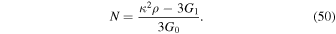
After obtaining these quantities, we can show the parameter space of the linear perfect fluid model in the reheating stage. By these equations, we can write the number of e-folds during reheating Nre, and the final reheating temperature Tre, in terms of the scalar spectral index ns. The results are shown in Figure 6. In this model, we adopt the value  from the ranges that are determined in Table 1. The behavior of the reheating processes of this model for
  coincides with the reheating results of the scalar field model with (V(ϕ) ∝ ϕ2) (Dai et al. 2014). The left panel of Figure 6 indicates the reheating e-folds number Nre, and the middle panel shows reheating final temperature Tre, versus the scalar spectral index ns, for various values of the EOS parameter
  . In this model, more wide ranges of the reheating e-folds number belong to
  and
and  , which is compatible with the Planck2018 data, i.e., these ranges indicate longer lifetimes than the others. The canonical reheating scenario, for
  , in the linear perfect fluid model has a shorter lifetime. The convergence point of all the lines in temperature plots, Figure 6(b), suggests the limit of
  , which presents the instantaneous reheating in each case. This temperature corresponds to the maximum temperature at the end of reheating. In this model, there is also more wide ranges of temperature for
  and
and  . In Figure 6(c), the e-folds number during reheating Nre versus the effective EOS parameter
  , shows the parameter space of reheating phase specified by the observational constraints, ns and r. Instantaneous reheating, equivalent to
  and
and  , is the point in which all of the curves converge together. In this figure, the colored region specified by requiring 0.9605 < ns < 0.9693 and r < 0.11, illustrates the allowed region for
  in the reheating process. The acceptable ranges of the number of e-folds and final temperature of the reheating stage for the linear perfect fluid model compared with Planck2018 observational data are summarized in Table 3.
Figure 6. (a) The reheating number of e-folds, and (b) the final reheating temperature, vs. the scalar spectral index ns, in the linear perfect fluid inflationary model. The horizontally highlighted regions represent T < 100 GeV with temperatures assumed to be below the electroweak scale and T < 10 MeV for with the temperatures assumed to be below the Big Bang nucleosynthesis scale and the vertically colored region shows the viable range of the scalar spectral index released by Planck2018 TT,TE,EE+LowE data. (c) The number of e-folds vs. the effective equation of state parameter  during the reheating phase. The colored region is the allowed region for
  that is specified by requiring 0.9605 < ns < 0.9693, r < 0.11 from Planck2018.
Download figure:
Standard image High-resolution imageTable 3. The Acceptable Ranges of the Number of e-folds and Final Temperature of the Reheating Stage for the Perfect Fluid Models (Linear and Exponential form), Compared with Planck2018 Observational Data
| Perfect Fluid | Linear Form | Exponential Form with β = 0.01 | Exponential Form with β = 0.001 | |||
|---|---|---|---|---|---|---|
| Nre | Tre (GeV) | Nre | Tre (GeV) | Nre | Tre (GeV) | |

|
N < 4.12 | T > 106.87 | N < 29.21 | T < 1014.93 | N < 24.05 | T < 1014.93 |
| ω = 0 | N < 7.56 | T > 10 3.35 | N < 58.49 | T < 1014.93 | N < 49.14 | T < 1014.93 |

|
N < 89.69 | T > 10−4 | N < 5.15 | 106.23 < T < 1014.93 | N < 21.65 | 10−3.42 < T < 1014.93 |

|
N < 45.02 | T > 10−4 | N < 2.74 | T > 1014.93 | N < 8.93 | 105.21 < T < 1014.93 |
| ω = 1 | N < 21.99 | T > 103.45 | N < 1.71 | T > 1014.93 | N < 4.81 | 1012.05 < T < 1014.93 |
Download table as: ASCIITypeset image
4.2. Reheating Phase with Exponential Perfect Fluid
In this subsection, we investigate the reheating process in an exponential form of the perfect fluid inflationary model. We present the additional constraints on inflationary parameters of this perfect fluid model by following plots that come from the reheating era. The number of e-folds in the exponential perfect fluid model defined as
Now, by using the Equations (31), (32), and (3), we find
and
We attempt to illustrate the parameter space of the exponential form of the perfect fluid inflationary model for β = 0.001 and β = 0.01, in the reheating stage. The results are shown in Figures 7 and 8, by the plots of Nre and Tre, versus the scalar spectral index ns. In these models, we use the logical values of G2 and G3, which are determined in Table 2. In these two cases, we adopt  and
and  for the values of (β = 0.001) and (β = 0.01), respectively. These results are close to the conclusions of the reheating processes in the scalar field inflationary model with V(ϕ) ∝ ϕ2, in Dai et al. (2014). For β = 0.01, it is clear in Figure 7(a), that most of the lifetime of this model belongs to the
  , and the canonical reheating, i.e,
  . The same conditions apply to the exponential model with β = 0.001, which is illustrated in Figure 8(a). The maximum temperature at the end of reheating (or the instantaneous reheating), in the exponential perfect fluid inflationary model, in both cases β = 0.001 and β = 0.01, correspond to the viable ranges of the Planck data in Figures 7(b) and 8(b). The wider range of acceptable final temperature, in both cases, is relevant to
  and
and  . The parameter space of the reheating phase, which is specified by the Planck data in Figures 7(c) and 8(c), shows wider ranges with respect to the linear perfect fluid model in the reheating epoch. The acceptable ranges of the number of e-folds and final temperature of the reheating stage for the exponential perfect fluid model with β = 0.001 and β = 0.01, compared with Planck2018 observational data are summarized in Table 3.

Figure 7. (a) The reheating number of e-folds, and (b) the final reheating temperature vs. the scalar spectral index ns, in the exponential perfect fluid inflationary model with β = 0.01. (c) The reheating number of e-folds vs. the effective equation of state parameter ωre , during the reheating phase for the exponential perfect fluid inflationary model with β = 0.01.
Download figure:
Standard image High-resolution image
Figure 8. (a) The reheating number of e-folds, and (b) the final reheating temperature, vs. the scalar spectral index ns, in the exponential perfect fluid inflationary model with β = 0.001. (c) The reheating number of e-folds vs. the effective equation of state parameter ωre, during the reheating phase for the exponential perfect fluid inflationary model with β = 0.001.
Download figure:
Standard image High-resolution image
5. Summary
In this paper, we have reviewed the inflation and reheating of reconstructed perfect fluid models. First, by examining the evolution of the slow-roll parameter , with respect to the inflationary parameters ρ and N, we were able to determine the constants G0 and G1 in the linear form and G2 and G3 in the exponential form of the perfect fluid models. We have explored the spectral index of curvature perturbations, the tensor-to-scalar ratio, and the running of the spectral index, in each of these models. Then, we have compared our results for linear and exponential forms of the perfect fluid with the recent Planck data. We have illustrated r − ns and αs − ns trajectories, for N = 50–70 and obtained some constraints on the model's parameter space. The recent data for observations on scalar spectral index ns and the tensor-to-scalar ratio r, which were suggested by Planck2018, are ns = 0.9649 ± 0.0044 (68% CL), r < 0.10 (95% CL), from Planck2018+TT,TE,EE+lowE+lensing. Additionally, the running of scalar spectral index is equal to αs = −0.0045 ± 0.0067, from the same Planck2018 data (68% CL). It can be seen from Equation (20) that when the condition  is realized in the inflationary era, we find (ns, r, αs) =(0.9649, 0.140, 3.08 × 10⁻⁴). The constraint on r with Planck2018+TT,TE,EE+lensing+lowEB relaxes to r < 0.16 (95% CL), so the value of r obtained by slow-roll conditions matches with observational data. In the linear form of perfect fluid in Equation (21), if
  and
and  , the value of ω(N) remains unchanged and conditions in Equation (20) can be met at the inflationary stage. Likewise, for the exponential form of perfect fluid in Equation (26), provided that β = 0.001 and hence βN ≪ 1, and that
  , then ω(N) can be regarded as constant and the conditions in Equation (20) can be satisfied during inflation. As a consequence, it is clear that perfect fluid models can lead to results corresponding to Planck2018 data. On the other hand, quantitative conclusions of the reheating phase of these inflationary models can match the end of the inflationary epoch with the beginning of the radiation-dominated phase of the universe with a perfect fluid component. The correlation between the number of e-folds during and after inflation determines the reheating e-folds number and the reheating final temperature. To study the reheating phase, we obtained the number of e-folds Nre, and final temperature Tre, during reheating in terms of the scalar spectral index ns, for different values of reheating effective EOS parameters
  , which is limited to physically reasonable values,
 ![$\left[-\tfrac{1}{3},1\right]$](https://content.cld.iop.org/journals/0004-637X/907/2/107/revision1/apjabcb80ieqn77.gif) . Our analysis shows that it is possible to have a viable reheating phase in these two models. In each case, we have explored the viable ranges of parameters in comparison with the Planck2018 data. It is obvious that the results obtained in the reheating era for each perfect fluid models are in good agreement with the recent observational data.
. Our analysis shows that it is possible to have a viable reheating phase in these two models. In each case, we have explored the viable ranges of parameters in comparison with the Planck2018 data. It is obvious that the results obtained in the reheating era for each perfect fluid models are in good agreement with the recent observational data.